Pairwise Document Similarity using an Incremental Approach to TF-IDF.

ABSTRACT

VENKATESH, JAYASHREE. Pairwise Document Similarity using an Incremental Approach to TF-IDF. (Under the direction of Dr. Christopher Healey.)

c

Copyright 2010 by Jayashree Venkatesh

Pairwise Document Similarity using an Incremental Approach to TF-IDF

by

Jayashree Venkatesh

A thesis submitted to the Graduate Faculty of North Carolina State University

in partial fulfillment of the requirements for the Degree of

Master of Science

Computer Science

Raleigh, North Carolina

2010

APPROVED BY:

Dr. Robert St. Amant Dr. Jon Doyle

DEDICATION

BIOGRAPHY

ACKNOWLEDGEMENTS

TABLE OF CONTENTS

List of Tables . . . vii

List of Figures . . . .viii

Chapter 1 Introduction . . . 1

1.1 Contributions . . . 2

1.2 Thesis Structure . . . 3

Chapter 2 A survey of Information Retrieval Systems . . . 4

2.1 Basic Algorithmic Operations . . . 6

2.1.1 Document Representation Techniques . . . 6

2.1.2 Information Retrieval Models . . . 8

2.2 Classic Information Retrieval Models . . . 10

2.2.1 Boolean (exact-match) Model . . . 10

2.2.2 Vector Model . . . 11

2.2.3 Probabilistic Model . . . 14

2.2.4 Comparison of the Classic Models . . . 17

2.3 Alternative Set Theoretic Models . . . 17

2.3.1 Extended Boolean Model . . . 17

2.3.2 Fuzzy Set Model . . . 19

2.4 Alternate Algebraic Models . . . 22

2.4.1 Generalized Vector Space Model . . . 22

2.4.2 Latent Semantic Indexing Model . . . 27

2.4.3 Neural Network Model . . . 30

2.5 Alternative Probabilistic Models . . . 32

2.5.1 Inference Network Model . . . 32

2.6 Structured Document Retrieval Models . . . 35

2.6.1 Non-Overlapping Lists Model . . . 35

2.6.2 Proximal Nodes Model . . . 36

Chapter 3 Document Similarity using Incremental TF-IDF . . . 39

3.1 Term-Weighing, Vector Space Model and Cosine Similarity . . . 41

3.1.1 Choice of Content Terms . . . 42

3.1.2 Term Weight Specifications . . . 43

3.2 Document Preprocessing . . . 45

3.2.1 Lexical Analysis of the Text . . . 46

3.2.2 Removal of Stop Words or High Frequency Words . . . 46

3.2.3 Suffix Stripping by Stemming . . . 47

3.3 Incremental Approach for TF-IDF Recalculation . . . 50

3.3.1 Term Weights and TF-IDF Data Structures . . . 50

3.3.3 Incremental TF-IDF . . . 51

Chapter 4 Results . . . 54

4.1 Handling Dynamic Document Collection . . . 55

4.1.1 Addition or Removal of Documents . . . 55

4.1.2 Calculating Document Similarity Difference . . . 55

4.2 Experimental Results . . . 57

4.2.1 Experiment Set-1 . . . 57

4.2.2 Experiment Set-2 . . . 60

4.2.3 Experiment Set-3 . . . 63

4.2.4 Experiment Set-4 . . . 65

4.3 Conclusion . . . 68

Chapter 5 Summary and Future Work . . . 70

5.1 Challenges and Future Directions . . . 71

LIST OF TABLES

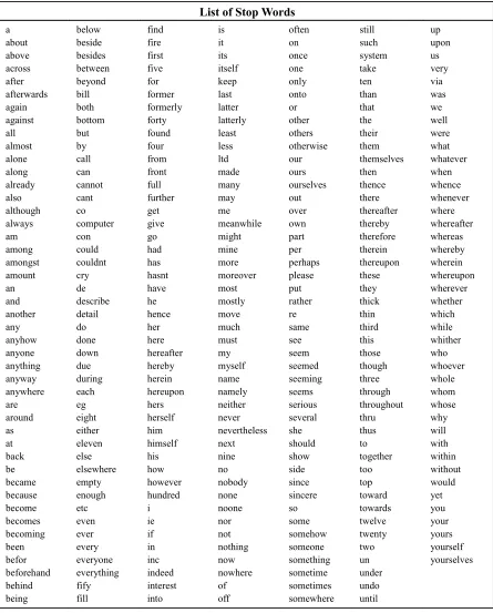
Table 3.1 Stop Words List . . . 48

LIST OF FIGURES

Figure 2.1 Extended Boolean Model: The map at the left shows the similarities of

qor= (kx∨ky) with documentsdj and dj+1. The map at the right shows

the similarities of qand= (kx∧ky) with documentsdj anddj+1. [6] . . . . 18

Figure 2.2 Neural Network Model [31] . . . 31

Figure 2.3 Inference Network Model [15] . . . 33

Figure 2.4 Non-Overlapping Lists Model [6] . . . 36

Figure 2.5 Proximal Nodes Model [32] . . . 37

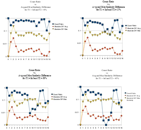
Figure 4.1 Graph of count ratio vs avg and max similarity difference for different document count difference thresholds . . . 58

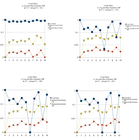
Figure 4.2 Graph of count ratio vs avg and max similarity difference for different percentage error thresholds . . . 61

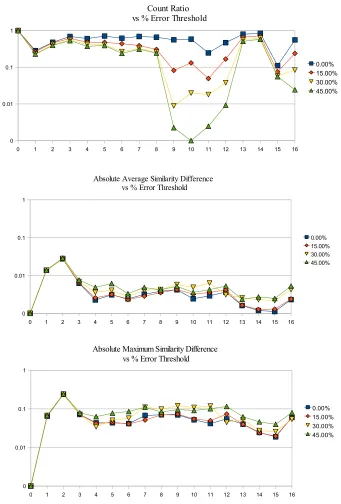
Figure 4.3 1) Count Ratio vs % Error Threshold 2) Average Similarity Difference vs % Error Threshold 3) Maximum Similarity Difference vs % Error Threshold 62 Figure 4.4 Graph of count ratio vs avg and max similarity difference for different percentage error thresholds . . . 64

Chapter 1

Introduction

The abundance of information (in digital form) available in on-line repositories can be highly beneficial for both humans and automated computer systems that seek information. This however poses extremely difficult challenges due to the variety and amount of data available. One of the most challenging analysis problems in the data mining and information retrieval domains is organizing large amounts of information [1].

While several retrieval models have been proposed as the basis for organization and retrieval of textual information,Vector Space Model(VSM) has shown the most value due to its efficiency. VSM however has substantial computational complexity for large set of documents and every time the document collection changes, the basic algorithm requires a costly re-evaluation of the entire document set. While in some problem domains it is possible to know what the document collection is a-priori, it is not feasible in many real time applications with large, dynamic set of documents.

higher the value of its term frequency [2]. Zipf [3] pointed out that a term which appears in many documents in the collection is not useful for distinguishing a relevant document from a non-relevant one. To take this into account the inverse document frequency (IDF) factor came into existence which determines the inverse of the relative number of documents that contain the term. A number of variations of TF-IDF exists today but the underlying principle remains the same [4].

VSM assigns a term weight to all the terms in a document. Thus a document can be represented as a vector composed of its term weights. Since there are several documents in the collection, the dimensionality of the vector space is equal to the total number of unique terms in the document collection. Pairwise document similarity computation is an important application of VSM which is based on the dot product of document vectors. On each addition or removal of a document to the collection, the document vectors will change. Specifically:

1. For terms in the document being added or removed, their IDF will change because of changes in both the number of documents containing the term, and the total number of documents.

2. For terms not in the document being added or removed, their IDF will also change because the total number of documents in the collection changes.

This means that with any change in the document set all the term weights associated with all the documents needs to be recalculated. To avoid recalculation of all the document vectors on each addition or removal of documents, we propose a mechanism to recalculate only a subset of the term weights and only when we estimate that the similarity error for deferring the calculation exceeds a predetermined threshold.

1.1

Contributions

addition or removal. We then modify the TF-IDF algorithm to perform recalculations of the term weights of only those terms whose document frequency changes on any change in the document set. We describe this as an incremental approach because unlike the traditional approach which recalculates all the TF-IDF values, recalculation is done only for a smaller set of terms.

Following this we conducted a series of experiments to determine how much reduction in the number of computations we achieved. For evaluation we use 1477 articles from various news-paper collections. We conducted our experiments on one of the most important applications of the VSM, pairwise document similarity calculation. We perform several steps of document ad-dition, removal or addition and removal. After each step we record the number of computations and the pairwise document similarity values as calculated by the incremental approach. We then run through the same set of steps with the traditional approach and once again record the number of computations made along with the document similarity values. We compare these values to evaluate the performance of the incremental approach as compared to the traditional approach. .

1.2

Thesis Structure

Chapter 2

A survey of Information Retrieval

Systems

The phenomenal growth in the variety and quantity of information available to users has resulted from the advances in electronic and computer technology. As a result users are often faced with the problem of reducing the amount of information to a manageable size, so that only relevant items can be examined. In Alvin Toffler’s bookFuture Shock [5], Emilio Segre, Nobel prize winning physicist, is quoted as saying that “on k-mesons alone, to wade through all the papers is an impossibility”. This indicates that even in specialized, narrow topics information is growing enormously. Thus a great demand for efficient and effective ways to organize and search through all the information is needed.

means by which authors or creators of records communicate with the readers, indirectly with a possible time lag between the creation of a text and its delivery to the IR system user.

IR can be subdivided into three main areas of research [8] which make up a considerable portion of the subject. Content analysis, information structures and evaluation.

Content analysis is concerned with describing contents of document in a form suitable for computer processing. Luhn [2], used frequency count of words to determine which words in a document should be used to describe the document. Spark Jones [9], used association of keywords (group of related words) to come up with frequency co-occurrence. This describes the frequency with which words occur together in a document. Several other content analysis techniques are in use today.

2.1

Basic Algorithmic Operations

Algorithmic issues arise in two aspects of IR systems: (1) representing objects (text/image/multimedia) in a form amenable to automated search, and (2) efficiently searching such representations [13].

First we shall focus on the various representations used for documents and information needs. We will then discuss the classic retrieval models for information retrieval.

2.1.1 Document Representation Techniques

Three classic ideas pervade information retrieval systems for efficient document representation. They are indexing, negative dictionaries (also known as “stop words”) and stemming [13].

A collection of documents is commonly referred to as a corpus. Indexing deals with storing the subsets of documents associated with different terms in the corpus. A simple query returns all documents which contain any of the query terms required. However, this approach leads to poor recall since a user generally requires a Boolean AND of the search terms and not the Boolean OR. To solve this issue we could retrieve the documents which match every query term and take an intersection of these set of documents. This approach would however process a lot more documents than what is returned as output. Hence, it is desirable for an efficient IR system to return a list of documents according to some ranking scheme based on the number of query terms the document contains. This however falls in the scope of retrieval models and will be discussed in the next section.

A better indexing mechanism is to store position of each occurrence of the term in the document along with the documents which contain the term. This would be helpful in case of queries dealing with a particular occurence of the query terms. Thus the indexing algorithm should be capable of supporting complex queries such as string queries. This suggests that it is necessary for the algorithm to understand the underlying corpus. Techniques that exploit the term statistics in the corpus were thus designed [13].

index term is not a good idea. This is because a query containing a term from the stop words list would fetch almost all documents in the corpus. Prepositions and articles are commonly included in the negative dictionaries. However usage of this technique has certain trade offs because it becomes difficult to search for certain strings that contain only prepositions and articles. Also, the contents of a negative dictionary should be designed keeping the corpus in mind - for instance the word “can” is generally considered a stop word, but in the case of waste management and recycling it might be an important index term.

Another important technique to reduce the number of index terms is the usage of a stem-ming algorithm. This approach reduces search and index terms to their etymological roots. For example, a search for ”educational” could return all documents containing the the term “education”.

Another approach could be to determine the lexical relationship between the terms in the query and the documents in which they occur [14]. If two terms appear adjacent to each other in a query and there are some documents which contain these two terms closer to each other (say within a distance of five-eight words), then the IR system could rank these documents higher than the others. For instance, a search for the term “computer networks” could return those documents first which contain these two terms closer to each other.

important task. Raghavan [13] talks about three important steps to consider before categorizing a corpus. First, the choice of categories should be intuitive to the anticipated user population. Secondly, the choice of categories should lead to a balanced taxonomy, in that a small number of categories containing all the documents is not recommended. Thirdly, the choice of categories should “span” the corpus. Choosing two categories that are very similar to each other is not desirable and could lead to confusion to the user.

It is also important to realize categorization of documents into clusters is not a static approach. In a corpus containing say news articles, the cluster may change as the focus of the news changes. Thus categorization should be dynamic and capable of supporting a rapid change in the documents contained in the cluster.

Finally, we bring back the idea of relevance feedback discussed at the beginning of this chapter. The IR system returns as output a set of documents based on the user’s query. The user then marks each of these documents as “relevant” or “irrelevant”. The system on receiving this input from the user now refines the query to fetch better results closer to what the user is seeking. This process leads to an increase in precision and recall.

2.1.2 Information Retrieval Models

While information can be of several types text, multimedia, images etc., most of the information sought by the end user is in the textual form. Several retrieval models have been proposed as the basis for text retrieval systems. However three classic models in IR which are used widely are called the exact match (Boolean) model, the vector space model and the probabilistic model. Recent experiments have shown that the differences in these approaches can be explained as the differences in the estimation of probabilities, both in the initial search and during relevance feedback [15].

as a measure of similarity. Thus this model is said to be algebraic. In the probabilistic model, retrieval is viewed as the problem of estimating the probability that a document representation matches or satisfies a query. As the name indicates this model is said to be probabilistic.

Several alternate modeling paradigms based on the classic models have been proposed in re-cent years. Fuzzy and extended boolean models have been developed as alternatives to the basic boolean approach. Generalized vector, latent semantic indexing and neural network models as alternatives to the algebraic models and inference networks and belief networks as alternatives to the probabilistic models [6].

While all these models deal with the text content found in documents several approaches dealing with the structure of the written text have also been proposed. These models are termed as structured models and two popular models in this category are the non-overlapping list model and the proximal nodes model.

are not discussed in this chapter.

2.2

Classic Information Retrieval Models

2.2.1 Boolean (exact-match) Model

Boolean model is a simple retrieval model based on set theory and Boolean algebra. In the Boolean model a set of binary valued variables refer to the features that can be assigned to the documents. A document is an assignment of truth values to this set of feature variables; features which are correct descriptions of the document content are assigned true and all other features are assigned false. As a result the weights assigned to the feature variables are all binary i.e., weightwi,j associated with the pair (ki, dj) is either 0 or 1. Herekiis theithfeature

variable anddj corresponds to thejth document.

In this model queries are specified as Boolean expressions involving the operators and, or

and not. Any document with truth value assignment that matches the query expression is said to match the query and all others fail to match. The Boolean model predicts that each document is either relevant or irrelevant. There is no notion of partial match to the query conditions.

2.2.2 Vector Model

The vector model [16, 17] realizes that the binary weighing scheme is too limiting and hence provides a framework where partial matching is possible. Thus the vector model works by assigning non-binary weights to the index terms in queries and in documents. These index term weights are now used to compute the degree of similarity between the documents in the corpus and also between the documents and the query. The similarity values are now used to sort the retrieved documents in decreasing order of the degree of similarity. Thus the vector model takes into consideration documents which match the query terms only partially. The documents retrieved as output now match the user’s query more precisely than the documents retrieved in the Boolean model.

In the vector model both the jth _{document d}

j and the queryq are represented as a

multi-dimensional vector. The vector model evaluates the similarity between the document dj and

the queryq. The correlation between the two vectorsd~j and~q is quantified as the cosine of the

angle between these two vectors. Thus similarity between the document vector and the query is given as:

sim(dj, q) =

~ dj·~q

|d~j| × |~q|

=

t X

i=1

wi,j ·wi,q

v u u t t X i=1 w_i,j2 ×

v u u t t X i=1 w2_i,q

(2.1)

where |d~j|and |~q| correspond to the length of the vectors and t is the number of dimensions.

While the query remains the same, the document space varies and hence normalization is essential. wi,j is weight associated with the pair (ki, dj), as indicated for the Boolean model

and is a positive non-binary term. The index terms in the query are also weighted. wi,q is the

(positive). Thus in this model both the documents and the query are represented as vectors with t index terms. The document vector is represented by d~j = (w1,j, w2,j, . . . , wt,j) and the

query vector by~q = (w1,q, w2,q, . . . , wt,q).

sim(dj, q) varies from 0 to +1 since bothwi,j andwi,qare positive. The vector model ranks

the documents according to their degree of similarity to the query instead of predicting whether the documents are relevant or not. Thus a document is retrieved even if it only partially matches a query. To prevent a large number of documents from being retrieved the user can specify a threshold for the similarity and only those documents which have a similarity value above the specified threshold will be retrieved.

Index term weights for the vector space model can be calculated in many different ways. However the most effective term weighing approaches use a clustering technique as described by Salton, Wong and Yang [18]. Thus the IR problem can be viewed as one of clustering. Given a collection of objects C and a user query with specification of a set A of objects, the clustering approach deals with classifying the objects in the collection C as belonging to the set A or not. The clustering approach deals with two issues. First, to identify what features better describe the objects in the set A. Second, to identify what features distinguish the objects in the set A from those not in the set A. Thus the two issues are to determine the intra-cluster similarity and the inter-cluster dissimilarity [6]. According to Salton and McGill [19], intra-cluster similarity can be measured by the frequency of a term ki in the document dj. This is referred to as the

term frequency (tf) and is a measure of how well the term determines the documents contents. For intra-cluster dissimilarity Salton and McGill [19], specify an inverse document frequency measure (idf). The idf factor indicates that the terms which appear in many documents are not very useful from distinguishing a relevant document from a non-relevant one. Thus an effective term weighing scheme tries to balance both these effects.

Let|D|be the total number of documents in a collection. Let|{d:ki∈d}|be the number of

documents in which the termki appears. Letf reqi,j be the frequency of the occurrence of the

dj). Then the normalized term frequency for the termki in the documentdj is given by

tfi,j =

f reqi,j t X

p=1 f reqi,j

(2.2)

where the denominator is the sum of the number of occurrences of all the terms in the document

dj. If the term ki does not appear in the document dj then the term frequencytfi,j = 0. The

inverse document frequency for the termki is given by

idfi = log

|D| |d:ki ∈d|

(2.3)

The best known term-weighing schemes use weights which use both the term frequency and the inverse document frequency.

wi,j =tfi,j×idfi (2.4)

The above term-weighing scheme is called as the TF-IDF weighing scheme. Salton and Buckley [20], suggest several variations for the weightwi,j, using the same underlying principle

2.2.3 Probabilistic Model

The probabilistic model was introduced by Robertson and Spark Jones [21], also known as the binary independence retrieval (BIR) model. The fundamental idea of this model is as follows. If the user query is known, there is a set of documents which contains exactly the relevant documents. This set of documents is known as the ideal answer set. Now, if the description of this ideal answer set is known, there is no problem in retrieving the set of relevant documents. However generally, the properties of this ideal answer set are not exactly known. Since the properties are unknown, at query time an initial guess is made as to what these properties could be. Through the probabilistic description of the ideal answer set, the first set of documents are retrieved. Now, the user through relevance feedback, looks at the retrieved documents to decide which documents are relevant and which ones are not. This helps in further improving the probabilistic description of the ideal answer set.

Given a query q and document dj, the probabilistic model tries to find the probability

that the user will find the documentdj relevant. The model assumes that there is a subset of

documents which the user prefers as the answer set to the queryq. Let us call this ideal answer set as the set R. The probabilistic model assigns to each document dj as its similarity to the

query q, the ratio P(dj being relevant to q)/P(dj non-relevant toq). This computes the odds

that the documentdj is relevant to the queryq.

Just as the boolean model, the index term weight variables for the probabilistic model are binary i.e., wi,j ∈ {0,1}, wi,q ∈ {0,1}. Query q is the subset of index terms. R is the set of

relevant documents and ¯R the set of irrelevant documents. Let P(R|d~j) be the probability that

the documentdj is relevant to the queryqand let P( ¯R|d~j) be the probability that the document

dj is non-relevant to the query q. The similarity measure of the documentdj with the query q

is defined as

sim(dj, q) =

P(R|d~j)

P( ¯R|d~j)

Using Bayes’ rule,

sim(dj, q) =

P(d~j|R)×P(R)

P(d~j|R¯)×P( ¯R)

(2.6)

where P(d~j|R) stands for the probability of randomly selecting the document dj from the set

of relevant documents R. P(R) is the probability that a document randomly selected from the entire collection is relevant. The meaning ofP(d~j|R¯) andP( ¯R) are analogous and

complemen-tary.

P(R) and P( ¯R) are the same for all documents in the collection. Thus we can write

sim(dj, q)∼

P(d~j|R)

P(d~j|R¯)

(2.7)

If we assume the independence of index terms (i.e., index terms are not related to each other), then we can rewrite Equation (2.7) as

sim(dj, q)∼

( Y

gi(d~j)=1

P(ki|R))×( Y

gi(d~j)=0

P( ¯ki|R))

( Y

gi(d~j)=1

P( ¯ki|R¯))×( Y

gi(d~j)=0

P( ¯ki|R¯))

(2.8)

where P(ki|R) stands for the probability that the index term ki is present in a document

randomly selected from the set R. P( ¯ki|R) is the probability that the index term ki is not

present in a document randomly selected from the set R. The meaning of P(ki|R¯) and P( ¯ki|R¯)

are analogous and complementary.

Now, initially we do not know the set R of retrieved documents. Hence it is essential to compute the probabilitiesP(ki|R) andP(ki|R¯). We make the following assumptions (1) assume

thatP(ki|R) is constant for all index terms (equal to 0.5) (2) also assume that the distribution

P(ki|R) = 0.5 (2.9)

P(ki|R¯) =

ni

N (2.10)

whereniis the number of documents which contain the index termkiandN is the total number

of documents in the collection. Using the Equations (2.9) and (2.10) we can now retrieve the initial set of documents which contain the query q and provide an initial probabilistic ranking for them. From here we further try to improve the ranking as follows.

Let V be the number of documents initially retrieved and ranked by the probabilistic model. Also, letVi be the subset of V which contains the index termki. To improve the probabilistic

ranking we need to improve P(ki|R) and P(ki|R¯). To achieve an improvement we now again

make the following assumptions (1) approximation ofP(ki|R) can be achieved by the

distribu-tion of the index terms ki among the documents retrieved so far (2) approximation ofP(ki|R¯)

can be done by considering that all non-retrieved documents are non-relevant. Now we can write,

P(ki|R) =

Vi

V (2.11)

P(ki|R¯) =

ni−Vi

N −V (2.12)

Now, the above process can be repeated recursively, which will improve the probabilities

P(ki|R) andP(ki|R¯).

2.2.4 Comparison of the Classic Models

From our discussion in the previous sections it is clear that the Boolean model is the weakest of all the classic models. Its main disadvantage being the inability to recognize the partial matches leading to poor performance. Experiments performed by Croft [15] suggest that the probabilistic model provides better performance than the vector model. However, experiments performed afterwards by Salton and Buckley [20] showed through several different measures that the vector model outperforms the probabilistic model with general collections. Thus the vector model is the most popular model used by researchers, practitioners and the web community.

2.3

Alternative Set Theoretic Models

Two alternate set theoretic models are popular. Namely the fuzzy set model and the extended Boolean model. In this section we discuss these two models in brief.

2.3.1 Extended Boolean Model

The extended Boolean model first appeared in the communications of the ACM article in 1983, by Salton, Fox and Wu [22]. In the boolean model for a query of the form q=kx ∧ky, only

a document containing both the index terms kx and ky are retrieved. There is no difference

between a document which contains either the term kx or the term ky or neither of them.

However, the extended Boolean model allows us to fetch even partially matching queries just as the vector space model. It combines both the vector space model and Boolean algebra to calculate the similarities between queries and documents.

Consider the scenario where only two terms (kx and ky) are present in the query. We can

now map the documents and queries in a two-dimensional map as shown in Figure 2.1. Weights

w1 andw2 are computed for the termskx andky respectively in the documentdj. The weights

Figure 2.1: Extended Boolean Model: The map at the left shows the similarities ofqor = (kx∨

ky) with documentsdj anddj+1. The map at the right shows the similarities ofqand= (kx∧ky)

with documentsdj and dj+1. [6]

w1=tfx,j×

idfx

maxiidfi

(2.13)

wheretfx,j is the term frequency (normalized) for the term kx in the documentdj,idfx is the

inverse document frequency for the termkx in the entire collection and idfi is the inverse

doc-ument frequency for a generic term ki. Similarly, the weight for the term ky can be calculated.

Now form the map shown at the left in Figure 2.1 we see that for the queryqor (kx∨ky), the

point (0,0) is the spot to be avoided, and form the map shown at the right in Figure 2.1 for the queryqand(kx∧ky), the spot (1,1) is the most desirable. This indicates that for the queryqor,

we take the distance from the spot (0,0) as a measure of similarity and for the queryqand, the

complement of the distance from the spot (1,1) as the measure of similarity. Thus we arrive at the formula:

sim(qor, dj) = r

w2₁+w2₂

2 (2.14)

sim(qand, dj) = 1− r

(1−w1)2+ (1−w2)2

The 2D Boolean model discussed above can be easily extended using Euclidean distances to include a document collection of a higher t-dimensional space. Thep-norm model can be used to include not only Euclidean distances but also p-distances where 1≤p≤ ∞.

Thus a generalized disjunctive query is given by:

qor =k1∨pk2∨p. . .∨pkm (2.16)

The similarity between qor and dj is given by:

sim(qor, dj) =

p s

wp_1,j+wp_2,j+. . .+wp_t,j

t (2.17)

A generalized conjunctive query is now given by:

qand=k1∧pk2∧p. . .∧pkm (2.18)

The similarity between qand anddj is given by:

sim(qand, dj) = 1−

p r

(1−w1,j)p+ (1−w2,j)p+. . .+ (1−wt,j)p

t (2.19)

More general queries such as q = (k1∧pk2)∨pk3 can easily be processed by grouping the

operators in a predefined order. The parameter p can be varied between 1 and infinity to vary the p-norm ranking behavior from vector based ranking to that of a Boolean like ranking (fuzzy logic). Thus the extended Boolean model is quite a powerful model for information retrieval. Though it has not been used extensively for information retrieval, it may prove itself useful later.

2.3.2 Fuzzy Set Model

elements have varying degrees of membership. In classical set theory membership of an element is assessed in binary terms, an element either belongs or does not belong to the set. This is called as a crisply defined set with every element holding the value of either 0 or 1. Fuzzy set theory allows gradual assessment of the membership of elements in a set (instead of abrupt). Fuzzy set is described with the aid of a membership function which is valued in the real interval [0,1].

A fuzzy set is thus a pair {A, m}whereAis a set andm:A→[0,1]. For eachx∈A, m(x) is called the grade of membership of x in {A, m}. Let x ∈ A. Then x is not included in the fuzzy set {A, m} if m(x) = 0, x is said to be fully included if m(x) = 1 and x is called fuzzy member if 0< m(x)< 1. The set{x∈ A|m(x)>0} is called the support of {A, m} and the set {x∈A|m(x) = 1} is called its kernel.

There are two classical fuzzy retrieval models: Mixed Min and Max (MMM) and Paice Model.

Mixed Min and Max Model (MMM)

In MMM model each index term has a fuzzy set associated with it. A document’s weight with respect to an index termA is the degree of membership of the document in the fuzzy set associated withA. Documents to be retrieved for a query of the form {A or B}, should be in the fuzzy set associated with the union of these two sets A and B. Similarly documents to be retrieved for a query of the form {A and B}, should be in the fuzzy set associated with the intersection of these two sets. Thus the similarity of a document to theor query ismax(wA, wB)

and similarity to the and query ismin(wA, wB). The MMM model tries to soften the boolean

operators by considering the query-document similarity to be a linear combination of the min and max document weights.

Thus given a documentdj and index term weightsw1, w2, . . . , wtfor termsk1, k2, . . . , ktand

qor = (k1 or k2 or . . . or kt) (2.20)

qand= (k1 and k2 and . . . and kt) (2.21)

the MMM model computes query doc similarity as follows:

sim(qor, dj) =Cor1×max(w1, w2, . . . , wt) +Cor2×min(w1, w2, . . . , wt) (2.22)

sim(qand, dj) =Cand1×min(w1, w2, . . . , wt) +Cand2×max(w1, w2, . . . , wt) (2.23)

where Cor1 and Cor2 are the softness coefficients for the or operator, and Cand1 and Cand2

are the softness coefficients for the and operator [23]. For an or term, we would like to give more importance to the maximum term weights and for an and term, more importance to the minimum term weights. Thus we have Cor1 > Cor2 and Cand1 > Cand2. For simplicity we

generally assumeCor1 = 1−Cor2 andCand1 = 1−Cand2.

Experiments conducted by Lee and Fox [24], show that best performance of the MMM model occurs withCand1 in the range [0.5, 0.8] and with Cor1>0.2. The computational cost of

the MMM model is generally low and retrieval effectives is generally better than the standard Boolean model.

Paice Model

sim(q, dj) = t X

i=1

ri−1×wi t X

j=1 rj−1

(2.24)

where r is a constant co-efficient and wi is the term weights arranged in ascending order for

and queries and descending order for or queries. When t= 2 the Paice model shows the same behavior as the MMM model.

Experiments by Lee and Fox [24], show that setting r = 0.1 for and queries and r = 0.7 foror queries gives good retrieval effectiveness. However, this method is more expensive when compared to the MMM model due to the fact that the term weights have to be sorted in ascending and descending order, depending on whether anand clause or anor clause is being considered. The MMM model only requires determination of min or max of a set of term weights hence can be done in O(t). The Paice model requires at least O(t×logt) for the sorting algorithm along with more floating point calculations.

Fuzzy set models have been mainly discussed in the literature dedicated to fuzzy theory and are not too popular among the information retrieval community. Also, majority of the experiments carried out has considered only smaller collections which make comparison difficult at this time.

2.4

Alternate Algebraic Models

Three alternate algebraic models are discussed in this section, namely, generalized vector space model, latent semantic indexing model, and the neural network model.

2.4.1 Generalized Vector Space Model

document vectors to compute a cosine similarity to rank the documents according to their degree of similarity with the query. The term frequency of the terms in a document is used to represent the components of the document vector. This model assumes that the term vectors are orthogonal i.e., for each pair of index terms ki and kj we have ki·kj = 0.

However, the terms in a document collection are generally correlated and an efficient IR model takes these term correlations into consideration. This interpretation led to the develop-ment of the generalized vector space model (GVSM) where the term vectors may be correlated and hence non-orthogonal.

In GVSM, the queries are presented as a list of terms with their corresponding weights. Thus GVSM cannot ideally handle Boolean queries (of the formAND,OR orNOT). However Wong, Ziarko, Raghavan and Wong [26], show that GVSM can also be extended to handle situations where Boolean expressions are used as queries.

Let (k1, k2, . . . , kt) be the set of index terms in a document collection. LetB2t be the set of

all possible Boolean expressions (also the number of possible patterns of term co-occurrence) using these index terms and the operators AND, OR and NOT. To represent every possible Boolean expression in B₂t as a vector in vector space, we need to have a set of basis vectors

corresponding to a set of fundamental expressions which can be combined to generate any element of the Boolean algebra. This leads to the notion of an atomic expression or a minterm. A minterm in t literals (k1, k2, . . . , kt) is a conjunction of literals where each termki appears

exactly once in either its complemented or uncomplemented form. Thus in all there are 2t minterms. The conjunction of any two minterms is always false (zero) and a Boolean expression involving (k1, k2, . . . , kt) can be expressed as a disjunction of the minterms.

~

m1 = (1,0, . . . ,0,0) (2.25)

~

m2 = (0,1, . . . ,0,0) (2.26)

..

. (2.27)

~

m2t = (0,0, . . . ,0,1) (2.28)

where each vector m~i is associated with the respective mintermmi. Now given these basic

vectors, the vector representation of any Boolean expression is given by the vector sum of the basic vectors. Notice that for all i 6= j, m~i·m~j = 0. Thus the set of m~i vectors is pairwise

orthonormal. If two vectors are not orthonormal then their corresponding Boolean expressions should have atleast one minterm in common.

To determine an expression for the index term vector k~i associated with the index term

ki let us use mi₂t to denote the set of all atomic expressions. Each term ki is an element of

Boolean algebra generated and can be expressed in the disjunctive normal form (sum of the vectors for all minterms) as:

ki =mi1 OR mi2. . . OR mip (2.29)

where mij’s are the minterms in which ki is uncomplemented and 1< j <2

t_{. If we denote}

the set of minterms in Equation (2.29) as mi_{, we can define the term k} i as

~ ki =

X

mr∈mi ~

mr (2.30)

or,

~ ki =

2t X

i=1

cirm~r (2.31)

cik = 

 

 

1 ifmr∈mi

0 otherwise

(2.32)

The term vectors are a linear combination of the mr’s i.e., the basic vectors and the vector

summation is theOR’s of Equation (2.29).

Now, let us recall the equations for the documents and the queries for the conventional vector space model. The documents and queries are represented by a set of vectors, say, {d~α|α= 1,2, . . . , p}, andq~. The normalized term vectors are represented as{k~i|i= 1,2, . . . , t}.

That is,

~ dα=

t X

i=1

aαik~i (α= 1,2, . . . , p) (2.33)

~ q=

t X

j=1

qjk~j (2.34)

where aαi is the weight assigned to the term ki in document dα and varies from 0 to 1 (i.e.,

0≤aαi≤1). Similarly qj is the weight of the termkj in the query q and varies from 0 to 1.

Using the above equations, we can deduce the similarity of the documents in {d~α}p and

query~q by the cosine of the angle betweend~α andq~which is given by the scalar product,d~α·~q.

~ dα·~q=

t X

i=1,j=1

aαiqjk~ik~j (α= 1,2, . . . , p) (2.35)

The higher the similarity value between a document and the query, the greater the relevance of the document to the query.

Let us express Equation (2.33) as follows:

D=kAT (2.36)

A=         

a11 a12 · · · a1t

a21 a22 · · · a2t

..

. ... . .. ...

ap1 ap2 · · · apt          (2.37)

Similarly, we could write Equation (2.35) as

S=qGAT (2.38)

where S= (d~1·~q, ~d2·~q, . . . , ~dp·~q) ,q = (q~1, ~q2, . . . , ~qt), and

G= (gij)         

k1·k1 k1·k2 · · · k1·kt

k2·k1 k2·k2 · · · k2·kt

..

. ... . .. ...

kt·k1 kt·k2 · · · kt·kt          (2.39)

In the conventional vector space model the term vectors are assumed to be orthogonal to each other. Thus the correlation matrix in Equation (2.39) becomes an identity matrix. That is,

gij =k~i·k~j 

 

 

1 ifi=j

0 ifi6=j

(2.40)

Thus with approximation G=I, the ranking matrix S can be re-written as

S =qAt (2.41)

we introduce a new operator, the “circle” sum operator (denoted by ⊕). Thus in GVSM, the documents are now represented as follows

~

dα=aα1k~1⊕aα2k~2⊕. . . aαtk~t

=⊕t

i=1aαik~i

(2.42)

where the circle sum⊕is defined as follows. Letk~r andk~sbe two term vectors having the form

suggested in Equation (2.30). Then,

~

kr⊕k~s= X

mv∈T

max(crv, csv)m~v (2.43)

where T = {m}r _{∪ {m}}s _{and 1 < r, s < t. The document vectors, d~’s are chosen such that}

there exists term correlation between the term vectors. In the situation where the terms are not correlated, i.e., k~r·k~s = 0 , there are no common basic vectors in the expansion of k~r and

~ ks.

Thus, we are now able to prove that the document representation using GVSM can be reduced to VSM easily. The ranking that results from GVSM combines the standard term-document weights with the correlations factors between the terms. However, it is still not clear in which situations GVSM outperforms the classic VSM. Also, the cost of computing the ranking in GVSM can be fairly higher for larger document collections because, in this case the number of active minterms may be proportional to the number of documents in the collection. Despite these drawback, the GVSM does introduce newer ideas which are important from theoretical point of view.

2.4.2 Latent Semantic Indexing Model

the answer set due to retrieval using index terms. Also, many relevant documents not related by any query terms may not be retrieved. These effects are mainly because of the vagueness associated with the retrieval process involving keywords [6]. The degree of similarity between a user query and a document may be poor due to the usage of different vocabulary to express the same concepts by the document author. Latent Semantic Indexing is one of the few approaches which tries to overcome this problem by taking into account synonymy and polysemy [27]. Synonymy refers to the fact that similar or equivalent terms can be used to express the same idea, and polysemy to the fact that some terms can have multiple unrelated meanings. If we do not consider synonymy, then many relevant documents may not be retrieved due to the over-estimate of dissimilarity. This leads to false negative matches. Ignoring polysemy on the other hand leads to erroneously matching several documents and the query. This in turn leads to false positive matches. Thus, LSI allows retrieval of a document which shares concepts with another document which is relevant to the query.

The main idea in the Latent Semantic Indexing model [28] is to map documents and query from a higher dimensional space into an adequate lower dimensional space. This is achieved by matching the index term vectors into a lower dimensional space. The claim is that the retrieval in the lower dimensional space is superior to that of the higher dimensional space. LSI applies Singular Value Decomposition (SVD) to the matrix oft index terms and n documents to reduce dimensionality. In SVD, a rectangular matrix is decomposed into the product of three other matrices [29]. One component matrix describes the original row entities as vectors of derived orthogonal factor values. Another matrix describes the original column values as vectors of derived orthogonal factor values. The third matrix, is a diagonal matrix containing scalar values such that when all the three component matrices are multiplied the original matrix is constructed.

LetA~ = (Aij) be a term document association matrix witht rows (number of index terms)

and n columns (number of documents). Each element of this matrix Aij is assigned a weight

weighing scheme as used for the classic vector space model. Now the matrixA~ is decomposed using singular value decomposition (SVD) as follows.

~

A=U ~~ΣV~T _(2.44)

whereU~ andV~ are orthogonal matrices andΣ is a diagonal matrix. The dimension of A is~

t×n. The non null elements of the matrix ~Σ are denoted asσ1, . . . σp wherep=min(t, n) and

σ1 ≥σ2≥. . .≥σp.

Now, to reduce the dimensionality only the k largest singular values of Σ are maintained.~ This is obtained by settingσi = 0 for alli > k. This is equivalent to reducingU~ and V~ to their

first k columns and ~Σ to its first k columns and rows. Instead of comparing the query to the n dimensional vectors representing the documents in the original space defined by A~, we now compare them in ak dimensional subspace defined byA~(k).

Thus we now have,

~

A(k) =U~(k)Σ(~k)V(~k)T (2.45)

The selection of value of k involves balancing of two opposing effects. Firstly, k should be large enough to fit all the structure of the original data. Secondly, k should be small enough to eliminate all the non-relevant representational details [30].

The relationship between any two documents in the reduced space of dimensionality k, can be computed from the A~(k)TA~(k) matrix given by

~

A(k)TA~(k) = (U~(k)Σ(~k)V(~k)T)T(U~(k)Σ(~k)V(~k)T)

=V~(k)Σ(~k)U(~k)TU~(k)Σ(~k)V(~k)T

=V~(k)Σ(~k)Σ(~k)V(~k)T)

= (V~(k)Σ(~k))(V~(k)Σ(~k))T

In the above matrix, the(i,j) element indicates the relationship between documentsdi and

dj. To rank documents with regard to a user query, we model the query as apseudo-document

in the original term-document matrix A~. For example, the query is modeled as the document with number 0. Thus in the matrix A~(k)TA~(k), the first row provides rank of all documents with respect to this query.

Thus the matrices used in Latent Semantic Indexing model are of rank k tand k n. They provide elimination of noise,removal of redundancy and hence form an efficient indexing scheme for the documents in the collection.

2.4.3 Neural Network Model

In an IR system, document vectors are compared to the query vectors to find the computation of a ranking, or the document vectors are compared to each other to estimate the degree of similarity between the documents. In either case, pattern matching is the basic operation performed. Neural networks are known to be good pattern matchers. Hence it is natural to use them as an alternative means for IR.

synonymous terms could also be activated.

d

d

d

d

_{. . . .}

_.

_{. .}

k

k

k

k

_{. . . .}

_.

_.

_.

_.

k

_{. .}

_.

q

q

q

Documents

Document Terms

Query Terms

Figure 2.2: Neural Network Model [31]

The query term nodes are initially assigned an activation level equal to 1(the maximum). These nodes then send the signal to the document term nodes where the signals are attenuated by the normalized query term weights w~i,q (as defined in the vector model). For instance

~ wi,q =

wi,q v u u t

t X

i=1 w2_i,q

(2.47)

document term weights w~i,j (again as defined in the vector model).

~ wi,j =

wi,j v u u t t X i=1 w2_i,j

(2.48)

Now, the signals which reach the document node are summed up. Thus, after the very first round of signal propagation, the activation level associated with the document nodedj is now

given by

t X

i=1 ~

wi,qw~i,j =

wi,qwi,j v u u t t X i=1 w_i,q2

v u u t t X i=1 w_i,j2

(2.49)

The above Equation (2.49) is exactly the same as the equation derived for the classic vector model. However, the neural network model does not stop at this point. The above process spread activation process continues, beyond the first round. This is similar to that of user providing relevance feedback after the first cycle. The process is allowed to continue until some threshold for the signal level is reached and then stops.

The neural network model is simple and efficient. Though not much experimentation is done to prove its efficiency when compared to the other models, especially for large document collections, it can still be used as an alternative IR model.

2.5

Alternative Probabilistic Models

2.5.1 Inference Network Model

dependence relations between these propositions.

The inference network shown in Figure 2.3 consists of two component networks: a document network and a query network. The document network represents the document collection. The document network is built once for a document collection. Its structure does not change during query processing. Random variables associated with a documentdtrepresents the event

of observing that document. Observation of a document causes an increased belief in the variables associated with its index terms. Index terms and document variables associated with a document are also represented as nodes in the network. Edges are directed from a document node to its index terms to indicate that observation of a network, yields improved belief on its term nodes.

d

d

d

d

k

k

k

. . . .

k

. . . .

q

q

_{. . . .}

I

Query Network

Document Network

AND OR

The query network consists of a single node which represents the user’s information need and one or more query representations which express that information need. A query network is built for each information need and is modified during query processing as existing queries are refined or new queries are added in an attempt to better characterize the information need. The document and query networks are joined by links between the document terms and the query representations. All nodes in the inference network are binary valued (true or false). Random variables associated with the user query models the event that information request specified by a query has been met. Random variables are also represented as a node in the query network.

The inference network described above is used to capture all the significant probabilistic dependencies between the variables (represneted as nodes) in the documents and the query networks. When the query is first built and attached to the document network, the belief associated with each node of the query network is computed. Initially the nodes representing the information need, are assigned a probability that the information need is met, given that no specific document in the collection has been observed and that all the documents in the collection are equally likely to be observed. Now, we observe a single document say di and

set di = true to all the nodes associated with document di. All other document nodes in the

network are set to false. We now try to compute a new probability that the information need is met given di = true. After this process is complete, we now remove the observation that

di = true and instead assign dj = true for some other document dj, j 6= i. This processs is

2.6

Structured Document Retrieval Models

Suppose the information need by a user is of the form “Macbeth’s castle”. And the user in this case is referring to a particular scene in Shakespeare’s play titled “Macbeth”. In the classic information retrieval model, all the documents containing this strings “Macbeth” and ”castle” would be retrieved. But the user is not interested in all the documents containing the above terms. The user is interested in only a specific part of the document satisfying his query. The user may also be interested in an interface with advanced options so he can specify his query needs precisely (eg, scene in the play). Thus, retrieval models which combine information on the text content with information on the document structure are called asstructured document retrieval models [6]. In this model, the system is expected to retrieve the most specific part of the document answering the user query (chapter, section, subsection etc.). Thus, a structured document retrieval model has two specific issues to deal with (1) which parts of the document to return to the user? (2) which parts of the document to index?

Two popular structured document retrieval models exist. They are the non-overlapping lists model and the proximal nodes model.

2.6.1 Non-Overlapping Lists Model

Chapter

Sections

Subsections

Sub sub sections L₃

L₂ L₁ L₀

Figure 2.4: Non-Overlapping Lists Model [6]

2.6.2 Proximal Nodes Model

This model, allows the definition of independent hierarchical indexing structures over the same document text. The indexing structure is hierarchical and is composed of chapters, sections, paragraphs, pages, lines and may be even sentences [32]. Each of these components correspond to a node type or a structural component. A text region is assigned to each node type (portion of text within that region). Thus, a hierarchy is a tree of structured nodes or simply (un-structured) nodes. Each node of the hierarchy belongs to a node type of the hierarchy and has an associated segment. A segment is a pair of numbers representing a contiguous portion of the underlying text. The pair of numbers refer to the beginning and ending positions of the text in that segment. Two different hierarchies may refer to the same overlapping text region.

Now, if a user query belongs to different hierarchies, the compiled answer is formed by nodes all of which come from only one of them. Thus, the result of a query cannot be composed of nodes from distinct hierarchies.

Consider a hierarchical indexing structure as shown in the Figure 2.5. Now, this structure consists of chapters, sections, subsections and subsubsections, along with an inverted list for the word “computer”. An inverted list is a list composed of two elements: the vocabulary and the occurrences [6]. Vocabulary is the set of all different words in the text and for each such word a list of all positions where the word appears is stored. This is called as the list of all word occurrences.

Chapter Chapter Chapter Book . .. . . .

. . . .

title

title

section section section figure

subsection title

title subsection subsection

Computer 15 45 250 . . . . 45000

. . . .

TEXT

.

.

.

.

Chapter 3

Document Similarity using

Incremental TF-IDF

Pairwise document similarity or document-document similarity refers to measurement of the association between each pair of documents in a document collection. By association we are trying to quantify the likeness or commonality between the pair of documents. Computing pairwise similarity on large document collections is a task common to a variety of problems such as clustering and cross-document co-reference resolution [33]. Measurement of pairwise document similarity is also critical for many text applications, e.g., document similarity search, document recommendations, plagiarism detection, duplicate document detection and document filtering [34].

similarities. Currently, however, most existing techniques measuring document similarity rely purely on the topical similarity measurements [34].

Document topic similarity aims at assessing to what extent two documents reflect the same topics. Existing topical similarity measurement techniques include cosine similarity, the Dice measure, the Jaccard measure, the Overlap measure, the information theoretic measure and the BM25 measure[8, 34]. Cosine similarity is the most popular of all these measures and is based on the vector space model (VSM). The Jaccard measure, the Dice measure and the Overlap measures are also based on the vector space model. All the VSM-based similarity measures mentioned here use term frequency and inverse document frequency (TF-IDF) for term weight calculations. Thus, TF-IDF calculations play an important role in document similarity measures.

The VSM relates terms to documents. Since different terms have different importance in a given document, each term is assigned a term weight [20]. In the TF-IDF approach term weights are computed from the frequency of a term within a document and its frequency in the corpus. To calculate the inverse document frequency, we need to know the number of documents that contain the term. This requires a priori knowledge of the data set, and also the assumption that the data set does not change after the calculation of the term weights. Thus most of the existing similarity models work under the assumption that the whole data set is available and is static.

However, many real-time document collections are dynamic and have continuous addition or removal of documents. For even a single addition or removal of a document, the document frequency value has to be updated for several terms, and all previously calculated term weights (TF-IDF values) need to be recalculated. Recall that the IDF for a termtiis the log of the total

number of documents in the collection divided by the number of documents that containti. Let

dj be a document which contains the term ti. When document dj is added or removed from

the document set, the number of documents containing ti changes. It increases by one if dj is

contains ti. Moreover, for even a single addition or removal, the total number of documents

changes. This affects every TF-IDF value in every document in the collection, even for terms that were not contained in documentdj. This leads to a worst case computational complexity

of O(N2P) to calculate the pairwise document similarity on each addition or removal of a document, where N is the number of documents in the collection, and P is the dimensionality of the term vectors.

In order to address the problem of TF-IDF computations for real-time document collections, we propose an Incremental TF-IDF approach. Our technique tries to limit the number of updates made to the TF-IDF values on addition or removal of documents by constraining the number of term weights that need to be recalculated.

In the remainder of this chapter we will explain the VSM in more detail and then move to the implementation details of the proposed solution.

3.1

Term-Weighing, Vector Space Model and Cosine Similarity

Vector space model assumes independence of terms. Each document is composed of term vectors of the form D = (t1, t2, . . . , tp) , where each tk identifies a constant term associated with the

document D. The terms (t1, t2, . . . , tp) are regarded as the coordinate axis in a p dimensional

coordinate system. Each term vector tk has a weight wk associated with it to specify the

importance of the term in that document. The term weights are vary from 0 and 1, with higher weight assignments used for more important terms.

Cosine similarity equates the similarity between two documents to the cosine of the angle between them their term vectors. Similarities ranges from 0 for completely dissimilar to 1 for completely similar. Given two documents with document attributes DI and DJ, the cosine

similarity is computed using the dot product of their term vectors as,

similarity(DI, DJ) = cos(θ) =

DI·DJ

|DI||DJ|

Thus if (wi1, wi2, . . . , wip) and (wj1, wj2, . . . , wjp) represent the term weights associated with

the documentsDI and DJ, then similarity of the two documents is given by,

similarity(DI, DJ) = p X

k=1

wik·wjk

v u u t

p X

k=1 w2_ik×

p X

k=1 w2_jk

(3.2)

In determining the cosine similarity of documents using the above equation, two main questions arise. First, what is an appropriate choice for the units to be used in document representations. Second, how can we construct term weights capable of distinguishing the important terms from less crucial ones [20].

3.1.1 Choice of Content Terms

In most commercial applications and early experiments, single terms alone were used for con-tent representation. These single terms are words extracted from the text of the documents. Recently, several enhancements in content analysis and text indexing have been proposed for the choice of content terms. These include the generation of sets of related terms, the formation of term phrases, the use of word grouping (or word classes) and the construction of knowledge bases [20].

which groups similar words together. Knowledge bases are structures designed to represent the subject area under consideration using techniques such as artificial intelligence. Entries from the knowledge bases are then used to represent the content terms of documents [20].

Each of the approaches suggested above as choices for content term representations are either inordinately difficult, not suitable for all types of document collections, or do not yet have viable procedures for successful implementation. Thus, single terms appear to be the best choice as content identifiers.

3.1.2 Term Weight Specifications

With single terms chosen for content identification, appropriate term weights have to assigned to the individual terms, to be able to distinguish the importance of one term from another. A term is said to have good indexing property if it improves the retrieval of relevant documents, while rejecting the non-relevant documents of a collection. These two factors relate to therecall

andprecisionmeasures of information retrieval systems, respectively. A good term is one which produces high recall by retrieving all relevant documents and also high precision by rejecting all unrelated documents [19].

Studies on document (indexing) space configurations have shown that a separated document space leads to a good retrieval performance [18]. Thus a good term is one which when assigned as an index term to a collection of documents will render the documents as dissimilar as possible. On the contrary, a poor term is one which renders the documents more similar and thus makes it difficult to distinguish one document from another. The idea is that, the greater the separation between the individual documents, and the more dissimilar the respective index terms are, the easier it is to retrieve some documents while rejecting others. This forms the basis of the term discrimination model [35].

term, it is sufficient to take the difference in the space densities before and after the assignment of the particular term. If the document space becomes more compact upon the removal of the termk, then the termk is said to be a good discriminator. This is because upon assignment of that term to the documents of a document collection, the documents will resemble each other less. The reverse is true for a poor discriminator [16].

The above study on assigning a weight to an index term based on its discrimination value leads to a relationship between the discrimination value of an index term and its document frequency . Document frequency (DF) is defined as the number of documents in the collection containing a particular index term. Terms with very low document frequencies, that may be assigned to just one or two documents are poor discriminators. This is because the presence or absence of these terms affect very few documents of the thousands of documents present in the collection. Similarly terms with very high DF that are assigned to several documents are also poor discriminators. The best discriminators are those terms whose DF is neither too high nor too low.

The above discussion on term discrimination, recall and precision leads to the following definition as term weights of single terms [20]

a) Terms that are frequently mentioned in individual documents, are useful for enhancing recall measures. This suggests that the term frequency factor (tf) be used as part of the term weighing system measuring the frequency of occurrence of the terms in the documents. The term frequency factor is usually computed as

tfi,j=

f reqi,j p X

m=1

f reqm,j

(3.3)

where f reqi,j is the frequency of the term ti in the document dj and the denominator is the

b) Term frequency alone cannot ensure good retrieval performance. If high frequency terms are not concentrated in a few documents, but instead are present in the entire document collec-tion, all documents tend to be retrieved, and this affects search precision. Hence, a collection dependent factor which favours terms concentrated in only a few documents of the collection needs to be used. This leads to the inverse document frequency (idf) factor. The idf factor varies inversely with the number of documentsn to which a term is assigned in a collection of

N documents. Thus idf factor is usually computed as,

idfi= log

N

n (3.4)

A reasonable measure of the term importance may be obtained by using the product of the term frequency and the inverse document frequency (tf×idf) [20]. This will assign the largest weight to those terms that have high frequencies in individual documents, but are at the same time relatively rare in the document collection as a whole. The weight of the term ti in the

documentdj is given by

wi,j =tfi,j×idfi (3.5)

3.2

Document Preprocessing

It is clear that not all terms are equally significant for expressing the semantics of a document. In written language, some words carry more meaning than others. Usually, noun words carry more meaning than other words and are most representative of a document content. Thus, preprocessing of the documents in the collection is essential to determine which words of the document to keep as index terms [6].

to be highly similar on the basis of words which have little or no meaning. Preprocessing the documents in a collection can be viewed as a process to control the size of the vocabulary.

The ultimate goal is the development of a text preprocessing system that employs com-putable methods and requires minimum human intervention to generate from the input text an effective retrieval system [8]. In our implementation we construct such a system using three steps 1) lexical analysis of the text 2) removal of stop words or high frequency words 3) suffix stripping by stemming.

3.2.1 Lexical Analysis of the Text

Lexical analysis is the process of converting a sequence of characters into a sequence of tokens or words. Generally, spaces are considered word separators. Lexical analysis involves grouping a sequence of non-space characters as tokens. Separation of digits, punctuation marks, hyphens and letters will also need to be considered [6].

Digits are generally not considered good index terms for a document. This is because numbers by themselves are normally vague. However numbers might prove to be useful index terms in many cases. For example, numbers representing the date of birth of an individual may be useful for hospital records, numbers representing customers’ driving license may be useful index terms for an insurance company, etc. Hence in our implementation we retain digits during lexical analysis. Punctuation marks and hyphens have no relevance to identifying documents and are normally removed. Letters are most commonly used as index terms. All letters are retained and are converted to lower case for consistency.

3.2.2 Removal of Stop Words or High Frequency Words

referred to as “stop words” and are normally discarded as potential index terms. This is done by comparing the input text to a “stop list” of words to be removed [8]. Articles, prepositions, and conjunctions are commonly considered stop words.

Removal of stop words has several other benefits. Stop word removal can reduce the number of index terms by 40% or more [6]. As a result the list of stop words is generally extended to include several verbs, adverbs and adjectives as well. Table 3.1 shows the list of stop words used in our implementation.

3.2.3 Suffix Stripping by Stemming

Natural language texts typically contain many different variations of a basic word. Morpholog-ical variants (e.g., connect, connected, connecting etc.) prevent exact match between words in two different documents. The effectiveness of matching two documents is expected to improve if it were possible to conflate (i.e., to bring together) the various variants of a word [36]. This can be performed by substituting words with their respective stems.

A stem is the portion of a word left after removing its affixes (i.e., prefixes and suffixes). In most cases only suffixes added at the right end of the word are removed. This is because most variants of a word are generated by the introduction of suffixes. The suffix stripping process will reduce the total number of terms in the IR system, and hence reduce the size and complexity of the data in the system [37].

Though several suffix stripping algorithms exists, the most widely used and efficient algo-rithm is the Porter’s stemming algoalgo-rithm [37], which uses an explicit list of suffixes together with the criterion under which a suffix may be removed from a word. The main benefits of Porter’s stemming algorithm is that it is small, fast, reasonably simple and yields results com-parable to those of more sophisticated algorithms. Because the algorithm is fast, it is applied to every word identified as an index term after the removal of stop words.

Table 3.1: Stop Words List

List of Stop Words