Design of a Stochastic Forecasting Model for Egg
Production
T. Jai Sankar
Department of Statistics, Bharathidasan University Tiruchirappalli – 620 024, Tamilnadu, INDIA
ABSTRACT
The egg has a very well balanced amino acid profile with the required minerals and vitamins. This paper deals with the design of the stochastic modeling for egg production forecasting in Tamilnadu, based on data on egg production during the years from 1996 to 2008. The study considered Autoregressive (AR), Moving Average (MA) and Autoregressive Integrated Moving Average (ARIMA) processes to select the appropriate stochastic model for egg production forecasting in Tamilnadu. Based on ARIMA (p, d, q) and its components ACF, PACF, Normalized BIC, Box-Ljung Q statistics and residuals estimated, ARIMA (0, 1, 1) was selected. Based on the chosen model, it could be predicted that the egg production would increase to 19,179 millions in 2015 from 8,960 millions in 2008 in Tamilnadu.
Keywords: Egg production, BIC, forecasting, ARIMA.
INTRODUCTION
Egg is food materials universally acceptable without being forbidden by any religious taboos. Egg is the cheapest food sources of animal protein. The egg has a very well balanced amino acid profile with the required minerals and vitamins. Unlike other animal fats, egg lipids are not fats; but oils good for health; they contain more omega-9 fatty acid-MUFA which increases the good HDL-cholesterol in the serum. Moreover, they contain considerable amounts of omega-3 fatty acids (N-3 PUFA) which reduces the serum bad LDL-cholesterol. Hence the egg and chicken lipids are good for health. Tamilnadu is one of the leading States in egg production and export. The eco-friendly backyard poultry rearing is practiced along with commercial poultry farming in the State. The egg production in the State which improved from 3784 million numbers in 2003-04 to 6395 million numbers in 2004-05 marginally declined to 6223 million numbers in 2005-06. Consequently the per capita availability of egg per annum has declined from 102 numbers. In this background, this study was conducted to forecast the future egg production in the State, so as to help the policy planners to formulate needed strategies for achieving and sustaining the targets in the sector.
MATERIAL AND METHODS
As the aim of the study was to forecast egg production, various forecasting techniques were considered for use. ARIMA model, introduced by Box and Jenkins (1970), was frequently used for discovering the pattern and predicting the future values of the time series data. Akaike (1970) discussed the stationary time series by an AR(p), where p is finite and bounded by the same integer. Moving Average (MA) models were used by Slutzky (1973). Hannan and Quinn (1979) suggested obtaining the order of a time series model by minimizing the errors for pure AR models, and Hannan (1980) for ARMA models. A second order determination method could be considered as a variance of Schwarz's Bayesian Criterion (SBC) which gives a consistent estimate of the order of an ARMA model. Hosking (1981) introduced a family of models, called fractionally differenced autoregressive integrated moving average models, by generalizing the ‘d’ fraction in ARIMA (p, d, q) model. Jai Sankar et al. (2010) used stochastic modeling for cattle production and forecast the yearly production of cattle in the Tamilnadu state during 1970-2010. Jai Sankar et al. (2011) also used stochastic modeling for bovine production and forecast the yearly production.
then first differences can be created. This is called second-order differencing. A distinction is made between a second-order differences (Yt-Yt-2).
While Mendelssohn (1981) used Box-Jenkins models to forecast fishery dynamics, Prajneshu and Venugopalan (1996) discussed various statistical modeling techniques viz., polynomial, ARIMA time series methodology and nonlinear mechanistic growth modeling approach for describing marine, inland as well as total fish production in India during the period 1950-51 to 1994-95. Tsitsika et al. (2007) also used univariate and multivariate ARIMA models to model and forecast the monthly pelagic production of fish species in the Mediterranean Sea during 1990-2005.
The time series when differenced follows both AR and MA models and is known as autoregressive integrated moving averages (ARIMA) model. Hence, ARIMA model was used in this study, which required a sufficiently large data set and involved four steps: identification, estimation, diagnostic checking and forecasting. Model parameters were estimated using the Statistical Package for Social Sciences (SPSS) package and to fit the ARIMA models.
Autoregressive process of order (p) is, Yt =
µ
+φ
1Yt−1+φ
2Yt−2 +....+φ
pYt−p +ε
t;Moving Average process of order (q) is, Yt =
µ
−θ
1ε
t−1−θ
2ε
t−2 −....−θ
qε
t−q +ε
t; and the general form of ARIMA model of order (p, d, q) ist q t q t t p t p t t
t
Y
Y
Y
Y
=
φ
1 −1+
φ
2 −2+
....
+
φ
−+
µ
−
θ
1ε
−1−
θ
2ε
−2−
....
−
θ
ε
−+
ε
where Yt is egg production export,
ε
t’s are independently and normally distributed with zero mean and constant varianceσ
2 for t = 1,2,..., n; d is the fraction differenced while interpreting AR and MA and φs and θs are coefficients to be estimated.Trend Fitting: The Box-Ljung Q statistics was used to transform the non-stationary data in to stationarity data and to check the adequacy for the residuals. For evaluating the adequacy of AR, MA and ARIMA processes, various reliability statistics like R2, Stationary R2, Root Mean Square Error (RMSE), Mean Absolute Percentage Error (MAPE), and Bayesian Information Criterion (BIC) [as suggested by Schwartz, 1978] were used. The reliability statistics viz. RMSE, MAPE, BIC and Q statistics were computed as below:
2 / 1 1 2
)
(
1
−
=
∑
= ∧ n i i iY
Y
n
RMSE
∑
= ∧−
=
n i i i iY
Y
Y
n
MAPE
1)
(
1
BIC(p,q) = ln v*(p,q) + (p+q) [ ln (n) / n ]
where p and q are the order of AR and MA processes respectively and n is the number of observations in the time series and v* is the estimate of white noise variance σ2.
) ( ) 2 ( 1 2 k n rk n n Q k i − + =
∑
=where n is the number of residuals and rk is the residuals autocorrelation at lag k.
In this study, the data on egg production in Tamilnadu were collected from the Department of Animal Husbandry and Veterinary Services, Government of Tamilnadu for the period from 1996 to 2008 and were used to fit the ARIMA model to predict the future egg production.
RESULTS AND DISCUSSION
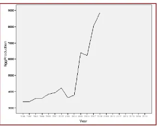
forecasting was a stationary series. The stationary series was the set of values that varied over time around a constant mean and constant variance. The most common method to check the stationarity is to explain the data through graph and hence is done in Figure 1.
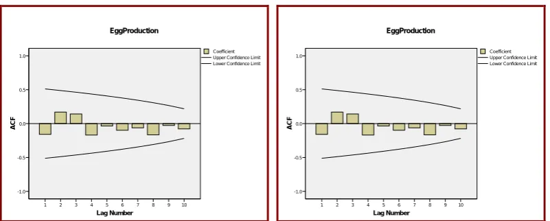
Figure 1 reveals that the data used were non-stationary. Again, non-stationarity in mean was corrected through first differencing of the data. The newly constructed variable Yt could now be examined for stationarity. Since, Yt was stationary in mean, the next step was to identify the values of p and q. For this, the autocorrelation and partial autocorrelation coefficients (ACF and PACF) of various orders of Yt were computed and presented in Table 1 and Figure 2.
Figure 1. Time plot of egg production in Tamilnadu
Table 1. ACF and PACF of egg production
Lag
Auto
Correlation Box-Ljung Statistic
Partial Auto Correlation
Value Df Sig. Value Df Value Df
1 -0.159 0.256 0.386 -0.159 0.256 -0.159 0.289 2 0.170 0.244 0.872 0.170 0.244 0.149 0.289 3 0.142 0.231 1.250 0.142 0.231 0.198 0.289 4 -0.169 0.218 1.849 -0.169 0.218 -0.157 0.289 5 -0.036 0.204 1.879 -0.036 0.204 -0.158 0.289 6 -0.098 0.189 2.150 -0.098 0.189 -0.102 0.289 7 -0.062 0.173 2.280 -0.062 0.173 0.002 0.289 8 -0.166 0.154 3.431 -0.166 0.154 -0.152 0.289 9 -0.027 0.134 3.472 -0.027 0.134 -0.077 0.289 10 -0.078 0.109 3.983 -0.078 0.109 -0.065 0.289
Lag Number 10 9 8 7 6 5 4 3 2 1 ACF 1.0 0.5 0.0 -0.5 -1.0 EggProduction
Lower Confidence Limit Upper Confidence Limit Coefficient Lag Number 10 9 8 7 6 5 4 3 2 1 ACF 1.0 0.5 0.0 -0.5 -1.0 EggProduction
Lower Confidence Limit Upper Confidence Limit Coefficient
The tentative ARIMA models are discussed with values differenced once (d=1) and the model which had the minimum normalized BIC was chosen. The various ARIMA models and the corresponding normalized BIC values are given in Table 2. The value of normalized BIC of the chosen ARIMA was 13.713.
Table 2. BIC values of ARIMA (p, d, q)
ARIMA (p, d, q) BIC values
(0, 1, 0) 13.868
(0, 1, 1) 13.713
(0, 1, 2) 14.029
(1, 1, 0) 13.934
(1, 1, 1) 14.031
(1, 1, 2) 14.375
(2, 1, 0) 14.228
(2, 1, 1) 14.372
(2, 1, 2) 14.733
Model Estimation: Model parameters were estimated using SPSS package and the results of estimation are presented in Tables 3 and 4. R2 value was 0.89. Hence, the most suitable model for egg production was ARIMA (0, 1, 1), as this model had the lowest normalized BIC value, good R2 and better model fit statics (RMSE and MAPE).
Table 3. Estimated ARIMA model of egg production
Estimate SE t Sig.
Constant -232817.421 61038.718 -3.814 0.004
MA 1 0.984 4.605 0.214 0.836
Table 4. Estimated ARIMA model fit statistics
Fit Statistic Mean
Stationary R-squared 0.510
R-squared 0.893
RMSE 696.300
MAPE 11.033
Normalized BIC 13.713
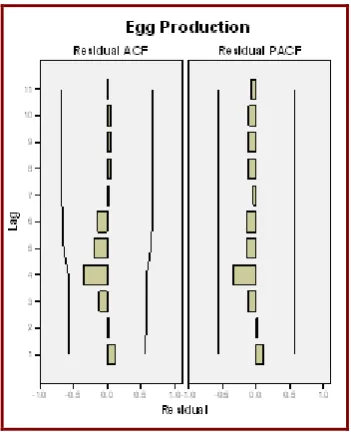
which has been done through examining the autocorrelations and partial autocorrelations of the residuals of various orders. For this purpose, various autocorrelations up to 11 lags were computed and the same along with their significance tested by Box-Ljung statistic are provided in Table 5. As the results indicate, none of these autocorrelations was significantly different from zero at any reasonable level. This proved that the selected ARIMA model was an appropriate model for egg production in Tamilnadu.
Table 5. Residual of ACF and PACF of egg production
Lag ACF PACF
Mean SE Mean SE
Lag 1 0.106 0.106 0.106 0.289
Lag 2 0.029 0.029 0.018 0.289
Lag 3 -0.121 -0.121 -0.127 0.289
Lag 4 -0.360 -0.360 -0.344 0.289
Lag 5 -0.194 -0.194 -0.149 0.289
Lag 6 -0.146 -0.146 -0.142 0.289
Lag 7 0.024 0.024 -0.044 0.289
Lag 8 0.051 0.051 -0.126 0.289
Lag 9 0.048 0.048 -0.128 0.289
Lag 10 0.050 0.050 -0.111 0.289
Lag 11 0.013 0.013 -0.081 0.289
The ACF and PACF of the residuals are given in Figure 3, which also indicated the ‘good fit’ of the model. Hence, the fitted ARIMA model for the egg production data was:
t t t
Y
=
−
232817
.
421
−
0
.
984
ε +
−1ε
Figure 3. Residuals of ACF and PACF
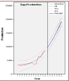
Forecasting: Based on the model fitted, forecasted egg production (in millions) for the year 2009 through 2015 respectively were 9737, 11019, 12418, 13933, 15565, 17314 and 19179 millions (Table 6). To assess the forecasting ability of the fitted ARIMA model, the measures of the sample period forecasts’ accuracy were also computed. This measure also indicated that the forecasting inaccuracy was low. Figure 4 shows the actual and forecasted value of egg production (with 95% confidence limit) in the State.
Year Actual Predicted LCL UCL
1996 3371 -- -- --
1997 3388 3139 1063 5216
1998 3584 3149 1350 4947
1999 3588 3295 1599 4991
2000 3845 3486 1844 5128
2001 3929 3792 2183 5401
2002 4223 4166 2580 5753
2003 3622 4641 3071 6212
2004 3784 5097 3539 6655
2005 6395 5651 4102 7199
2006 6223 6542 5001 8083
2007 8044 7446 5912 8981
2008 8860 8546 7017 10075
2009 -- 9737 8212 11261
2010 -- 11019 9494 12544
2011 -- 12418 10893 13943
2012 -- 13933 12409 15458
2013 -- 15565 14042 17089
2014 -- 17314 15792 18836
2015 -- 19179 17657 20700
Figure 4. Actual and estimate of egg production
The most appropriate ARIMA model for egg production forecasting was found to be ARIMA (0, 1, 1). From the forecast available from the fitted ARIMA model, it can be found that the egg production would increase to 19,179 millions in 2015 from 8,960 millions in 2008 in Tamilnadu. That is, using time series data from 1996 to 2008 on egg production, this study provides evidence on future egg production in the State, which can be considered for future policy making and formulating strategies for augmenting and sustaining egg production in the State.
REFERENCES
Akaike H. 1970. Statistical Predictor Identification. Annals of Institute of Statistical Mathematics 22: 203-270.
Alan Pankratz. 1983. Forecasting with univariate Box–Jenkins models - concepts and cases. John Wiley, New York, Page 81.
Box G E P and Jenkins J M. 1970. Time Series Analysis - Forecasting and Control. Holden-Day Inc., San Francisco.
Hannan E J and Quinn B G. 1979. The determination of the order of an autoregression. Journal of Royal Statistical Society B(41): 190-195.
Hannan E J. 1980. The estimation of the order of an ARMA process. Annuals of Statistics 8: 1071-1081. Hosking J R M. 1981. Fractional differencing. Biometrika 68(1): 165-176.
Jai Sankar, Prabakaran R, Senthamarai Kannan K and Suresh S. 2010. Stochastic Modeling for Cattle Production Forecasting. International Journal of Modern Mathematics and Statistics 4(2): 53-57.
Jai Sankar, Prabakaran R, Senthamarai Kannan K and Suresh S. 2011. Stochastic Modeling for Bovine Production Forecasting. International Journal of Agricultural and Statistical Sciences 7(1): 141-148. Mendelssohn R. 1981. Using Box-Jenkins models to forecast fishery dynamics: identification, estimation and checking. Fishery Bulletin 78(4): 887-896.
Prajneshu and Venugopalan R. 1996. Trend analysis in all India marine products export using statistical modeling techniques. Indian Journal of Fisheries 43(2): 107-113.
Slutzky E. 1973. The summation of random causes as the source of cyclic processes. Econometrica
5:105-146.