Two Software Normal Basis Multiplication Algorithms for GF(2n)

(1)

Two Software Normal Basis Multiplication Algorithms for GF(2

n

)

Haining Fan and Yiqi Dai

Abstract -

In this paper, two different normal basis multiplication algorithms for software

implementation are proposed over GF(2

n

). The first algorithm is suitable for high complexity

normal bases and the second algorithm is fast for type-I optimal normal bases and low complexity

normal bases. The ANSI C source program is also included in this paper.

Index Terms -

Finite field, normal basis, multiplication algorithm.

1. Introduction

The arithmetic operations in GF(2

n

) play an important role in coding theory, computer algebra,

and cryptosystems. Among the different types of field representations, normal basis (NB) has

received considerable attention for efficient implementation. For portability as well as for price

reasons, it is often advantageous to realize cryptographic algorithms in software. While many

constructions of VLSI NB multipliers have been proposed recently, few software-efficient NB

algorithms can be found in the open literature. In [1], a software algorithm for type-I optimal

normal bases (ONB) was presented. It can be further improved if the symmetric property

proposed in [2,3] is employed. In [3], Reyhani-Masoleh and Hasan proposed a word-level NB

multiplication algorithm over GF(2

n

), and we denote it as the RH algorithm. The RH algorithm is

designed for working with all NBs. A bit-level NB multiplication algorithm is presented in the

IEEE standard P1363-2000 [4], but it is not efficient for software implementation. Ning and Yin

presented a generalized version of this algorithm in [5], and we denote it as the NY algorithm.

Although the NY algorithm is fast for ONBs, it is slow for nonoptimal normal bases.

__________________________

Haining Fan and Yiqi Dai are with the Department of Computer Science, Tsinghua University, Beijing 100084,

People's Republic of China.

(2)

In this paper, two NB multiplication algorithms for software implementation are proposed. The

first algorithm (Algorithm 1) is an improvement on the RH algorithm. The theoretical analysis

shows that it is faster than the RH algorithm. But experimental results show that this is not true for

a few GF(2

n

)s, e.g. GF(2

359 ) and GF(2

491 ). The reason is that the size of lookup tables of

Algorithm 1 is larger than that of the RH algorithm. The total number of cyclic shift operations

(CSO) needed in the second algorithm (Algorithm 2) is a constant. For type-II ONBs, the NY

algorithm is faster than Algorithm 2, but it is slower than Algorithm 2 for other NBs. Compared to

Algorithm 2, Algorithm 1 is suitable for high complexity NBs. For example, our experimental

results show that it is faster than Algorithm 2 in GF(2

283 ) (Type 6 Gaussian NB (GNB)) and

GF(2

571 ) (Type 10 GNB).

We also compare these NB algorithms to the polynomial basis multiplication algorithm

presented in [6], i.e., the finite field analogue of the Montgomery multiplication for integers. Our

experimental results show that in some GF(2

n

)s where ONBs or low complexity normal bases

exist Algorithm 2 is faster than the Montgomery algorithm, for example, type 4 GNBs in GF(2

577 ),

GF(2

673 ) and GF(2

739 ).

This paper is organized as follows: Section 2 introduces the RH algorithm and presents a

method to reduce the number of cyclic shift operations. This method may be applied to all NB

multiplication algorithms we discussed. Algorithm 1 and Algorithm 2 are presented in Section 3

and Section 4 respectively. Theoretic analyses and numerical results are presented in Section 5.

Finally, concluding remarks are made in Section 6.

2. Preliminaries

Let

be an element of GF(2

n

), for simplicity, denote

2

i

by

_i

. Given a normal basis

N=

{

₀

,

₁

,

₂

,...,

_n₁

}

of GF(2

n

) over GF(2), a field element A can be represented by a binary

vector (a0,a1,...,a

n-1

) with respect to this basis as

1

0

n

i i i

a

A

, where

a

i

GF

(

2 )

and i = 0,1,...,n-1.

For

1 i

n

1 , let

1 0

, 0

n

j j j i

(3)

j

i,

GF(2). Let

S

i

j

|

i, j

1 and h

i

=|S

i

|. We may rewrite S

i

as

S

i

{

w

i,1

,

w

i,2

,...,

w

i,hi

}

, where

1 ...

0 w

_,₁

w

_,₂

w

_,

n

i h i i

i

. (1)

Clearly,

i

k i h k w i 1 0 ,

.

Note that for a particular normal basis N the representation of

₀

_i

is fixed and so is w

i,k

.

In [3] a vector-level normal basis multiplication algorithm over GF(2

n

) is presented. The

algorithm includes two similar versions: one is for n odd and the other is for n even. In this paper,

we assume that n is odd, unless otherwise stated.

Let v=(n-1)/2 and <x> denote the non-negative residue of x mod n. D=AB can be computed by

the following identity [3]:

1

0

1

0 n

i

j

i

j

n

j

i

b

a

AB

D

1

2

0

1

0

1

0

1 (

)

n

i

j

n

j

i

n

i

j

b

a

b

a

v

i

h

k

n

j

w

j

i

j

i

n

i

i k i

a

b

a

b

a

1

0

1

0

1

_,

. (2)

Let A

i

=

i

A

2 . If we define B & A

n-i

as B & A

n-i

=

(

a

i

b

0 ,

a

i

1 b

1 ,...,

a

i

n

1 b

n

1 )

and treat it as the

field element, then

k i k

i

n

i

w

n

j

w

j

i

b

B

A

a

, ,

)

&

(

1

0 . So (2) may be rewritten as follows:

D

v i h k w i n w i n i k i k

i

A

B

A

B

A

B

1 1

1

&

,

&

,

&

(3)

v

i k S

k i n i n i

B

A

B

A

B

1

&

. (4)

Furthermore, Let R

i

=(B & A

n-i

)+(A & B

n-i

), we have

D=(B & A)

1+

v

i k S

k i i

R

1

)

(

. (5)

Similarly, for even n, we set v= n/2 and have:

D=(B & A)

1+

v

i k S

k i i

R

1

)

(

, (6)

(4)

v v

i n i

n i

B

A

R

v

i

B

A

B

R

&

1

1 where

)

&

(

)

&

(

_{. (7)}

Based on (5), the following multiplication algorithm was presented in [3]:

RH Multiplication Algorithm for n odd:

INPUT: A, B, S

i

, where

1 i

v

.

OUTPUT: D=AB.

S1: D := (A & B) >> 1;

S2: U

A

:= A; U

B

:= B;

S3: for i = 1 to v do {

S4: U

A

:= U

A

<< 1 ; U

B

:= U

B

<< 1;

S5: R := (A & U

B

)

(B & U

A

);

S6: for each

k

S

_i

do D := D

(R >> k); }

S7: Output D ;

Notes: 1. A & B=

(

a

₀

b

₀

,

a

₁

b

₁

,...,

a

_n

₁

b

_n

₁

)

.

2. denotes the addition in GF(2

n

).

3. A<<i (resp. A>>i) denotes i-fold left (resp. right) CSO of the coordinates of A.

Obviously, the number of CSO in S4 is n-1. Before introducing the first algorithm, we show

that this number can be further reduced for large values of n.

Let z be the full width of data-path of the general-purpose processor, e.g. z=32 for Pentium

CPU. We assume that z<v.

Let DA

0 = (a

0 ,a

1 ,...,a

n-1

,a

0 ,a

1 ,...,a

v-1

) and DA

j

= (a

j

,...,a

n-1

,a

0 ,a

1 ,...,a

v-1

a

0 ,...,a

j-1

), i.e., DA

j

is the

j-fold left cyclic shifts of the (n+v)-bit vector DA

0 , where 0<j<z .

In software implementation, DA is defined as a 2-dimensional array DA[z][

z v

n

_{], and each}

DA

j

is stored in

n_zv

successive computer words. So for

1 i

v

, A

n-i

is stored in

z n

successive computer words starting from DA[s][t] and ending at DA[s][t+

z

n

_{-1], where t=[i/z],}

s=i && (z-1) and && denotes integer bit-wise AND. That is to say, the two indices of A

n-i

can be

(5)

address of A

n-i

may be calculated in the precomputation procedure. Similarly, arrays DB

j

's are

defined.

Clearly, the time complexity to compute DA

j

's and DB

j

's (

0 j

z

) is about 3z n-bit CSOs,

and 3zn bits are needed to store these arrays.

3. Algorithm 1

Now we present the first algorithm. It is an improvement on the RH algorithm. The idea is

based on the following observation on (5). For some

1 i

₁

...

i

_e

v

,

e

i

S

₁

...

may not be

empty. Thus for each

e

i

S

k

₁

...

,

e i

i i

i k S

k i

R

,..., 1

)

(

can be computed by

e i

i i

i k S

k i

R

,..., 1

)

(

=

k i i i i e

R

,..., 1

. (8)

The saving of the k-fold cyclic shift operation is obvious. The left side of (8) needs e such

operations, while the right side needs only 1.

The correctness of this method is based on the fact that we can interchange the order of

summation in the identity (5). That is to say, since

0 k

n

1 , we have

D=(B & A)

1+

v

i k S

k i i

R

1

)

(

k n

k i i v k S

i i

R

A

B

1

0 : such that 1 and 1

&

. (9)

Similarly, for even n, we set v= n/2 and have:

D=(B & A)

1+

v

i k S

k i i

R

1

)

(

k n

k i i v k S

i i

R

A

B

1

0 : such that 1 and 1

&

. (10)

where R

i

is defined in (7).

Based on (9) and the method to compute DA

i

and DB

i

for 0<i<z, we now present Algorithm 1

for odd values of n. For each

0 k

n

1 , the following precomputation procedure is to find all i's

such that

1 i

v

and

i

S

k

.

Precomputation:

INPUT: n, S

i

, where

1 i

v

.

(6)

S1: for k = 0 to n-1 do e

k

:=0;

S2: for i = 1 to v do {

S3: for each

k

S

_i

do {

S4: m[k][e

k

] := i ;

S5: e

k

:= e

k

+1; } }

This procedure outputs e

k

and m[k][j], where

0 k

n

1 and

0 j

e

_k

1 . e

k

is the total

number of i's such that

1 i

v

and

k

S

_i

, and m[k][0] to m[k][e

k

-1] store these i's, i.e.,

] ][ [k j m

S

k

for

0 j

e

k

1 .

Multiplication Algorithm 1 for n Odd:

INPUT: A, B, e

k

and m[k][j], where

0 k

n

1 and

0 j

e

k

1 .

OUTPUT: D=AB.

S1: Compute DA

i

and DB

i

for

0 i

z

;

S2: D := A1

& B

1;

S3: for i = 1 to v do R[i] := (B & A

n-i

)

(A & B

n-i

);

S4: for k = 0 to n-1 do

S5: if e

k

> 0 then{

S6: C := R[m[k][0]];

S7: for j = 1 to e

k

-1 do C :=C

R[m[k][j]];

S8: D := D

(C >> k); }

S9: Output D ;

Notes: Algorithm 1 may be implemented without computing arrays DA and DB. In this

implementation, each R[i] is computed using statements similar to S4 and S5 of the RH algorithm

[5], and the total number of CSO becomes at most 2n. Experimental results indicate that arrays

DA and DB speedup Algorithm 1 by no more than 10% for GF(2

n

)s listed in Table 4 of Section 5.

For example, Algorithm 1 without computing arrays DA and DB performs one multiplication

(7)

4. Algorithm 2

From the definition of A&B we know that

(A & B)

i

=

i

B

A

_&

₎

2

(

=

(

a

_n

_i

b

_n

_i

,

a

_n

_i

₁

b

_n

_i

₁

,...,

a

_n

₁

b

_n

₁

,

a

₀

b

₀

,...,

a

_n

_i

₁

b

_n

_i

₁

)

=(A

i

& B

i

).

Thus (3) can be rewritten as:

D

v i h k i w w i w w i k i k i k i k

i

A

B

A

B

1 1 1

1

&

,

&

, ,

&

_,

. (11)

Since

₍

₁

₎

_/

₂

1

N v

i

C

h

, D can be computed by (11) at the cost of about C

N

AND (&) and C

N

XOR (

) operations if A

i

's and B

i

's are available, where 0<i<n and C

N

denotes the complexity of

the normal basis N.

Now we show that (11) can be further improved. From (1) we know that

₀

₁

,

n

w

ik

and

t i s

i

w

, ,

for a given i, where

1 i

v

and

1 s

t

h

i

. Thus (11) can be rewritten as:

1 0 1 where , some for that 1 and such : 1 1 ,

&

n w h k k w

w i i v

i w w i w w i k i

B

A

B

A

B

D

1 0 1 where , some for and 1 that such : 1 where , some for and 1 that such : 1 1 , ,

&

n w h k k w w v i i i w w h k k w w v i i i w w i k i i k i

A

B

A

B

. (12)

Obviously, the number of & operations in (12) is 2n+1. Thus (12) is faster than (11) for

nonoptimal normal bases.

Similarly, for even n, we set v= n/2 and have:

D

v k v k v i k i k i k i k i h k v w w v i h k i w w i w

w

B

A

B

A

B

1 1 1 1 1

1

&

,

&

, ,

&

, ,

&

_,

.

1 0 1 where , some for that 1 1and such : 1 where , some for that 1 and such : 1 1 , ,

&

n w h k k w

w i i v

i w w h k k w

w i i v

i w w i k i i k i

A

B

A

B

. (13)

Especially, for type-I ONBs, it is well known that

₁

₍

₂

₎

0 v

GF

and

0 i

j

for some

1

0 j

n

, where

1 i

v

1 . Thus the formula (13) can be further simplified if the Hamming

(8)

v v

i

i w w

i w

w

A

B

A

B

A

B

D

i i

i

&

HammingWe

ight

&

1 1 1

1 ,1 ,1 ,1 _,₁

. (14)

A

w

=A

n-(n-w)

can be computed by the method introduced in Section 2. Here the array DA is

defined as:

DA

0 = (a0,a1,...,a

n-1

,a0,a1,...,a

n-1

) and

DA

j

= (a

j

,...,a

n-1

,a

0 ,a

1 ,...,a

n-1

a

0 ,...,a

j-1

), where

1 j

z

,

i.e., they are 2n-bit vectors. The array DB is defined in the similar way.

So the time complexity to compute DA

j

and DB

j

is about 4z n-bit cyclic shift operations, and

4zn bits are needed to store these arrays, where

0 j

z

.

Based on (12), we now present the second algorithm for odd values of n.

For each

0 w

n

1 , the following precomputation procedure is to find all i's such that

v

i

1 and w=w

i,k

for some k, where

1 k

h

_i

.

Precomputation:

INPUT: n, S

i

, where

1 i

v

.

OUTPUT: e

w

and m[w][j], where

0 w

n

1 and

0 j

e

_w

1 .

S1: for w = 0 to n-1 do e

w

:=0;

S2: for i = 1 to v do {

S3: for each

w

S

_i

do {

S4: m[w][e

w

] := i ;

S5: e

w

:= e

w

+1; } }

This procedure outputs e

w

and m[w][j], where

0 w

n

1 and

0 j

e

_w

1 . e

w

is the total

number of i's such that

1 i

v

and w=w

i,k

, and m[w][0] to m[w][e

w

-1] store these i's, i.e.,

] ][ [w j m

S

w

for

0 j

e

_w

1 .

Multiplication Algorithm 2 for n Odd:

INPUT: A, B, e

w

and m[w][j], where

0 w

n

1 and

0 j

e

_w

1 .

(9)

S1: Compute DA

i

and DB

i

for

0 i

z

;

S2: D := A1

& B

1;

S3: for w = 0 to n-1 do

S4: if e

w

> 0 then{

S5: UA := A<w-m[w][0]>; UB := B<w-m[w][0]>;

S6: for j = 1 to e

w

-1 do { UA := UA

A

<w-m[w][j]>; UB := UB

B

<w-m[w][j]>; }

S7: D := D

(B

w

& UA)

(A

w

& UB); }

S8: Output D ;

Notes: For each

0 w

n

1 , A

w

=A

n-(n-w)

is stored in

n_z

successive computer words starting from

DA[s][t] and ending at DA[s][t+

_zn

_{-1], where t = [(n-w)/z], s = (n-w) && (z-1) and && denotes}

integer bit-wise AND. In our implementation, these address computations are performed in the

precomputation procedure, and starting addresses of A

w

, A<w-m[w][j]>, B

w

and B<w-m[w][j]> are stored

sequentially in a 1-dimensional array for

0 w

n

1 .

5. Analysis and Comparison

We implement these algorithms in ANSI C using Microsoft Visual C++ 6.0 complier and test

them on two computers:

1. An IBM ThinkPad 770X notebook with a 300 MHz Pentium II CPU running Windows NT

4.0. 2. A PC compatible computer with a 450 MHz Pentium III CPU running Windows 2000.

Both experimental results serve to validate our conclusions based primarily on theoretical

considerations. Timings listed in this paper are obtained on the first computer.

We call the RH algorithm using precomputation tables DA and DB the improved RH algorithm.

The time complexity of the original RH algorithm is determined in [3]. It needs n n-bit AND

operations and

2

1

2

1 C

N

n

₌

₍

_C

_n

₂

₎

_/

₂

N

n-bit XOR operations. The number of n-bit CSO of the

original RH algorithm is equal to

(

C

_N

2 n

1 )

/

2 . While the original and improved RH algorithms

(10)

z

C

_N

3

2 )

1 (

_{CSO. Thus it is faster than the original RH algorithm when n>3z+1.}

Now we determine the time complexity of Algorithm 1. Since

₍

₁

₎

_/

₂

1

0

N v

i i n

k

h

C

e

, the total

number of XOR in line S7 and S8 is

₍

₁

₎

_/

₂

N

C

. Thus the total number of XOR operations in

Algorithm 1 is

2

1

2

1 C

N

n

₌

2 /

)

2 (

C

_N

n

. Obviously, Algorithm 1 requires n AND operations. Thus

the two RH algorithms and Algorithm 1 require the same number of XOR and AND operations.

It is well known that

_C

_2n

₁

N

, thus the total number of CSO in the improved RH algorithm is

at least n+3z. Since e

k

may be zero for some k's, one can see that the total number of CSO in

Algorithm 1 is at most n+3z. Obviously, Algorithm 1 is faster than the improved RH algorithm for

nonoptimal normal bases.

For

₀

_i

_n

₁

, let

1 0

, 0

n

j

j j i

i

be the expansion of

0 i

with respect to the normal

basis generated by

, where

₍

₂

₎

,j

GF

i

. The following matrix was defined in [7].

1 0

, 1 0 , 0

n j

n i j i

T

(15)

For type-II ONB, the matrix T0 defined for the type-II optimal normal basis is symmetric. So

we know that the probability of e

k

=0 is 0.25 for type-II ONBs in Algorithm 1. Our experiments

show that for 100<n<1000, where n is odd and type-II ONB exists in GF(2

n

), the minimal,

average and maximal percentages that e

k

=0 are 22.9%, 25.0% and 27.2% respectively. That is to

say, the average total number of CSO in Algorithm 1 is (3n/4)+3z. So Algorithm 1 should be faster

than the improved RH algorithm for type-II ONBs. But numerical results show that this is only

true for small values of n, e.g. 131, 233 and 293. The reason is that the size of temporary variables

of Algorithm 1 is larger than that of the improved RH algorithm. In fact, while about 3zn/8 Bytes

are needed to store arrays DA and DB in both algorithms, approximately n

2 /16 Bytes are needed to

store R

i

's (

1 i

v

) in statement S3 of Algorithm 1. This large array increases the transfer from the

(11)

Since computation of starting addresses of A

w

, A

<w-m[w][j]>

, B

w

and B

<w-m[w][j]>

in Algorithm 2 may

be performed in the precomputation procedure, it is easy to determine the time complexity of

Algorithm 2, i.e. 4z CSO, 2n AND and C

N

XOR operations.

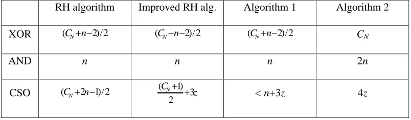
Table 1 compares the time complexity of these NB algorithms for nonoptimal normal bases in

GF(2

n

) where n is odd.

TABLE 1: Comparison of NB multiplication algorithms for nonoptimal normal bases.

RH algorithm

Improved RH alg.

Algorithm 1

Algorithm 2

XOR

(

C

_N

n

2 )

/

2 (

C

_N

n

2 )

/

2 (

C

_N

n

2 )

/

2 C

N

AND

n

2n

CSO

(

C

_N

2 n

1 )

/

2 C

N

₃

z

2 )

1 (

< n+3z

4z

We assume that the general-purpose processor can perform 1 n-bit XOR or AND using 1 n-bit

operation. As defined in [3], we also assume that 1 CSO needs

n-bit operations. Our

experiments and [3] show that the value of

is typically 4 for the C programming language if

only simple logical instructions, such as AND, SHIFT and OR are used to emulated a k-fold cyclic

shift. When

=4 and z=32, we may deduce the following condition that Algorithm 1 is faster

than Algorithm 2: C

N

> 7n - 256. Thus for high complexity NBs, Algorithm 1 is theoretically the

fastest one among these NB algorithms. The experimental results listed in Table 4 confirm this

conclusion.

Now we compare Algorithm 2 to the NY algorithm for type-I ONBs.

A bit-level NB multiplication algorithm was presented in the IEEE standard P1363-2000 [4].

Ning and Yin proposed a generalized version of this algorithm in [5]. The NY algorithm is very

fast for ONBs, but it is slow for nonoptimal normal bases. The difference between Algorithm 2

and the NY algorithm is that a different multiplication matrix is used, i.e., Algorithm 2 uses the

matrix T0 defined in (15) and the NY algorithm uses the matrix M defined in Annex 6.3 of [4].

(12)

Hamming weight. The Hamming weight of A can be computed by a lookup table. For example, if

we create a table with 2

8 entries on a 32-bit computer, our experimental results show that the cost

to compute A's Hamming weight is no more than 4 times that of a field addition operation for

n=162, 418 and 562.

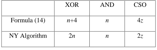
Since no description of the precomputation procedure was presented in [5] (part of the NY

algorithm was described in a patent application), we assume that the method introduced in Section

2 is used to perform this precomputation procedure. For the NY algorithm, DA

j

and DB

j

are

defined as z

n

_z

-bit vector, thus the total number of CSO is about 2z. Based on this assumption, it

is easy to see that the fastest NY algorithm, Algorithm 4 of [5], requires about 2n bit XOR, n

n-bit AND and 2z n-n-bit CSO. Thus the theoretical analysis shows that formula (14) is faster than the

NY algorithm for n>260 if we assume that

=4 and z=32. Our experiments confirm this

conclusion. Table 2 compares the time complexity of formula (14) and the fastest NY Algorithm

for type-I ONBs. Timings of some type-I ONBs are listed in Table 3.

TABLE 2: Comparison of Formula (14) and the fastest NY Algorithm for type-I ONBs.

XOR

AND

CSO

Formula (14)

n+4

n

4z

NY Algorithm

2n

n

2z

TABLE 3: Timing for some type-I ONBs (

s

)

GF(2

162 )

GF(2

226 )

GF(2

292 )

GF(2

418 )

GF(2

562 )

Formula (14)

31

49

67

122

195 NY Algorithm 4

31

49

69

136

216 We now compare these NB algorithms to the polynomial basis multiplication algorithm

presented in [6], i.e., the finite field analogue of the Montgomery multiplication for integers.

Since this method is significantly faster than the standard polynomial basis multiplication

(13)

implement the multiplication algorithm in GF(2

k

) instead of GF(2

n

), where

w n

w

k

. From [6]

we know that the case w=8 results in the fastest implementation on modern 32-bit computers. So

we also select w=8, and employ the table lookup approach, which is shown to be the best choice

to perform word-level multiplications [6].

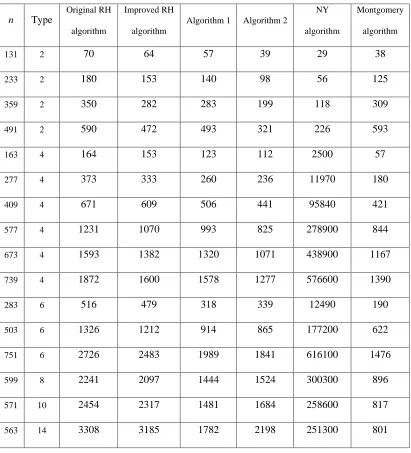
Experimental results are listed in Table 4. The 5 binary fields recommended by NIST for

ECDSA applications are GF(2

163 ), GF(2

233 ), GF(2

283 ), GF(2

409 ) and GF(2

571 ).

TABLE 4: Timing for some GF(2

n

)s (

s

)

n

Type

Original RH

algorithm

Improved RH

algorithm

Algorithm 1

Algorithm 2

NY

algorithm

Montgomery

algorithm

131

2

70

64

57

39

29

38

233

2

180

153

140

98

56

125

359

2

350

282

283

199

118

309

491

2

590

472

493

321

226

593

163

4

164

153

123

112 2500

57

277

4

373

333

260

236 11970

180

409

4

671

609

506

441 95840

421

577

4 1231

1070

993

825 278900

844

673

4 1593

1382

1320

1071

438900

1167

739

4 1872

1600

1578

1277

576600

1390

283

6

516

479

318

339 12490

190

503

6 1326

1212

914

865 177200

622

751

6 2726

2483

1989

1841

616100

1476

599

8 2241

2097

1444

1524

300300

896

571

10 2454

2317

1481

1684

258600

817

563

14 3308

3185

1782

2198

251300

801 Table 4 shows that for some GF(2

n

)s where type 4 GNBs exist, Algorithm 2 is faster than the

(14)

algorithm. So for applications where many squaring operations are needed, e.g. exponentiation,

Algorithm 2 is a better choice.

6. Conclusions

We have presented two normal basis multiplication algorithms in GF(2

n

). Algorithm 1 is

suitable for high complexity NBs and Algorithm 2 is fast in GF(2

n

) where type-I ONBs or low

complexity NBs exist.

7. Acknowledgments

(15)

References

[1] Haining Fan, "Simple Multiplication Algorithm for a Class of GF(2

n

),"

Electronics Letters, vol. 32, No.7, pp.636-637, 1996.

[2] A. Reyhani-Masoleh and M.A. Hasan, "On Efficient Normal Basis Multiplication,"

In LNCS 1977 as Proceedings of Indocrypt 2000, pp.213-224, Calcutta, India, December 2000.

Springer Verlag.

[3] A. Reyhani-Masoleh and M.A. Hasan, "Fast Normal Basis Multiplication Using General

Purpose Processors," Technical Report CORR 2001-25, Dept. of C&O,

University of Waterloo, Canada, April 19, 2001.

[4] IEEE P1363-2000. "Standard Specifications for Public Key Cryptography," August 2000.

[5] P. Ning and Y.L. Yin, "Efficient Software Implementation for Finite Field Multiplication in

Normal Basis," In LNCS 2229 as Proceedings of 3rd International Conference on Information

and Communications Security (ICICS) 2001, pp.177-188, Xian, China, 2001. Springer Verlag.

[6] C. Koc and T. Acer, "Montgomery multiplication in GF(2

k

),"

Design,Codes and Cryptography, vol. 14, No.1, pp.57-69, Apr. 1998.

[7] R.C. Mullin, I.M. Onyszchuk, S.A. Vanstone, and R.M. Wilson, "Optimal normal bases in

GF(p

n

)," Discrete Applied Mathematics, vol. 22, pp.149-161, 1988/89.

[8] S. Gao and Jr. H.W. Lenstra, "Optimal Normal Bases,"

Design,Codes and Cryptography, 2:315-323, 1992.

[9] J. Lopez and R. Dahab. "High-Speed software multiplication in F(2

m

),"

Technical report, IC-00-09, May 2000. Available at

(16)

//Since the eprint accepts only .ps and .pdf, I put the ANSI C source program here: /*////////////////////////////////////////////////////////////////////////// //

// This file is used to test performance of multiplication algorithms. //

// Author: Haining Fan // Date: MAY 2003 //

// Usage: 1. Create a sample "Hello, world!" Win32 Console Application nb; // 2. Replace nb.cpp with this file;

// 3. Build nb.exe in Release mode.

// 4. You may change the definition of N and TEST_NUM_OF_MUL. // 5. Other changes should be made carefully.

//

// Source code for testing ONB1 algorithms is also included in this file. //

///////////////////////////////////////////////////////////////////////////*/ #include "stdafx.h"

#include <time.h> #include <sys/timeb.h> // You may change N

#define N 283 // N odd #if (N==131)

#define T 2

#define TAIL_MASK (0x7) // = (2**(N- (N/W)*W)) - 1 #endif

#if (N==233) #define T 2

#define TAIL_MASK (0x1ff) #endif

#define TAIL_MASK (0x7f) #endif

#define TAIL_MASK (0x7) #endif

#define TAIL_MASK (0x1fffff) #endif

#define TAIL_MASK (0x1ffffff) #endif

(17)

#define TAIL_MASK (0x7fff) #endif

#define TAIL_MASK (0x7fffff) #endif

#define TAIL_MASK (0x7ffff) #endif

#define ln_xor2(a, b) for (zqa=0; zqa<DWSZ; zqa++) a[zqa] ^= b[zqa];; #define ln_zero(a) for (zqa=0; zqa<DWSZ; zqa++) a[zqa]=0;;

#define ln_and(a, b, c) for (zqa=0; zqa<DWSZ; zqa++) a[zqa] = b[zqa] & c[zqa];; #define ln_copy(a, b) for (zqa=0; zqa<DWSZ; zqa++) a[zqa] = b[zqa];; #ifndef BYTE

typedef unsigned char BYTE; #endif

#ifndef WORD

typedef unsigned short WORD; #endif

#ifndef DWORD

typedef unsigned long DWORD; #endif

#define W 32

#define TAIL_SZ (N- (N/W)*W) #define P (T*N+1) #define V ((N- 1)/2) #define DWSZ ((N/W) + 1) // for Montgomery #define BLK_SZ 8 #if ((N % BLK_SZ) == 0) #define MBLK_NUM ((N/BLK_SZ)+1) #else

#define MBLK_NUM ((N/BLK_SZ)+2) #endif

// You may increase the value of TEST_NUM_OF_MUL if your computer is a faster one. #if (P>2000)

#define TEST_NUM_OF_MUL 1000 #else

#define TEST_NUM_OF_MUL 10000 #endif

void precomputation_of_Montgomery(); void precomputation_of_RH_and_me(); void precomputation_of_NY(); void ln_ror_once(DWORD *p); void ln_rol_once(DWORD *p); void ln_ror(DWORD *p, int count);

void ln_xor_ror(DWORD *r, DWORD *a, int count); // NB mul alg.

void original_RH_mul(DWORD * c, DWORD * a, DWORD * b); void improved_RH_mul(DWORD * c, DWORD * a, DWORD * b); void our_Alg_1(DWORD * c, DWORD * a, DWORD * b); void our_Alg_1_for_ONB2(DWORD * c, DWORD * a, DWORD * b); void our_Alg_1_without_DA_DB(DWORD * c, DWORD * a, DWORD * b); void our_Alg_2(DWORD * c, DWORD * a, DWORD * b);

(18)

// PB mul alg.

void Montgomery(BYTE * c, BYTE * a, BYTE * b); // tables used by the NY alg.

int tb_NY_t1[N], tb_NY_t2[N], tb_NY_M[N*N]; // tables used by the Montgomery alg.

BYTE TBL[65536], TBH[65536]; WORD TBN[MBLK_NUM];

// tables used by the RH and our alg.

int tb_RH_h[N], tb_RH_w_1D[T*N], tb_FD_e[N]; int tb_FD[T*N], tb_FD_i[N];

DWORD * tb_FD_pab[2*T*N+N];

DWORD * tb_FD_m_1D[T*N], tb_FD_r[V+2][DWSZ]; DWORD * tb_FD_m_1Dua[T*N];

DWORD * tb_FD_m_1Dub[T*N];

DWORD zua[32][2*DWSZ], zub[32][2*DWSZ]; int main(int argc, char* argv[]) {

DWORD bb[1+DWSZ], aa[1+DWSZ], vv[1+DWSZ], uu[1+DWSZ]; DWORD sss=0xabcdef21, seed=0x87654321;

int i, j, num=0;

int qq1=0, qq2=0, qq3=0, qq4=0; int qq5=0, qq6=0, qq7=0, qq8=0; struct timeb tt1, tt2;

precomputation_of_RH_and_me(); precomputation_of_Montgomery(); precomputation_of_NY();

printf("End of precomputation. N=%d T=%d", N, T); /*

// used to check correctness. for(;;)

{

ftime(&tt1); for(i=0; i<DWSZ; i++)

bb[i]=seed=tt1.millitm+tt1.time*sss + ((seed * (0xefabd67^seed) )>>3); for(i=0; i<DWSZ; i++)

vv[i]=seed=tt1.millitm+tt1.time*sss + ((seed * (0xefabd67^seed) )>>3); improved_RH_mul(aa, bb, vv);

our_Alg_2(uu, vv, bb); j=0;

for(i=0; i<=DWSZ- 2; i++) if (aa[i] != uu[i]) j++; if ( 0 != ((aa[DWSZ- 1]^uu[DWSZ- 1])<<(32- TAIL_SZ)) ) j++; if (j>0) printf("Error !!\ n");

} */ for(;;)

{ num++;

for(i=0; i<DWSZ; i++)

uu[i]^=seed=tt1.millitm+tt1.time*sss + ((seed * (0xefabd67^seed) )>>3); for(i=0; i<DWSZ; i++)

vv[i]=seed=tt1.millitm+tt1.time*sss + ((seed * (0xefabd67^seed) )>>3); printf("\ n\ nmultiplication performance (run %d times): \ n", TEST_NUM_OF_MUL); ftime(&tt1);

for(j=0; j<TEST_NUM_OF_MUL; j++)original_RH_mul(aa, uu, vv); ftime(&tt2);

if (tt2.millitm<tt1.millitm) {(unsigned short)tt2.millitm+=1000;(long)tt2.time--;} qq1 += 1000*(tt2.time- tt1.time) + tt2.millitm- tt1.millitm;

printf("original RH %d ms; ", qq1/num); ftime(&tt1);

for(j=0; j<TEST_NUM_OF_MUL; j++)improved_RH_mul(aa, uu, vv); ftime(&tt2);

printf("improved RH %d ms; ", qq3/num); ftime(&tt1);

for(j=0; j<TEST_NUM_OF_MUL; j++)our_Alg_1_without_DA_DB(aa, uu, vv); ftime(&tt2);

(19)

if (T==2){// is ONB2 ftime(&tt1);

for(j=0; j<TEST_NUM_OF_MUL; j++)our_Alg_1_for_ONB2(aa, uu, vv); ftime(&tt2);

}else{ ftime(&tt1);

for(j=0; j<TEST_NUM_OF_MUL; j++)our_Alg_1(aa, uu, vv); ftime(&tt2);

}

printf("\ nAlg.1 %d ms; ", qq4/num); ftime(&tt1);

for(j=0; j<TEST_NUM_OF_MUL; j++)our_Alg_2(aa, uu, vv); ftime(&tt2);

printf("Alg.2 %d s; ", qq6/num); ftime(&tt1);

for(j=0; j<TEST_NUM_OF_MUL; j++) Montgomery((BYTE*)aa, (BYTE*)uu, (BYTE*)vv); ftime(&tt2);

printf("Montgomery %d ms; ", qq5/num); if (T==2){// is ONB II

ftime(&tt1);

for(j=0; j<TEST_NUM_OF_MUL; j++)Alg3_of_NY_for_ONB2(aa, uu, vv); ftime(&tt2);

}else{

printf("\ nFor nonONB, the NY alg. is slow and we run it only %d times: ",\ TEST_NUM_OF_MUL/100);

ftime(&tt1);

for(j=0; j<TEST_NUM_OF_MUL/100; j++)Alg2_of_NY(aa, uu, vv); ftime(&tt2);

}

printf("NY %d ms; ", qq7/num); // printf("\ n");

} return 0; }

int tb_tmp_w[V+2][N], tb_tmp_F[P], tb_tmp_m[N][N]; // these are local variables. void precomputation_of_RH_and_me()

{

int w, n, i, j, k, u, f; BYTE a[N], b[N], c[N]; // find a primitive mod P

u=1; next:

u++; j=1;

for(i=1; i <= P- 2; i++){ j = (j*u) % P; if (j==1) goto next; }

// here u is primitive mod P j=u;

for(i=1; i < N; i++) u = (u*j) % P; // now, u is an int of order T mod P, where P=TN+1; // get F(1..P)

w=1;

for (j=0; j<T; j++) { n=w;

for (i=0; i<N; i++) { tb_tmp_F[n] = i; n = (n<<1) % P; }

w = (u*w) % P; }

(20)

for (k=1; k<=V; k++){

for (j=0; j<N; j++) c[j]=a[j]=b[j]=0; w=0; u=k;

a[0]=b[k]=1; // A=Beta; B=Beta^(2^k) for (i=0; i<N; i++){

for (n=1; n<=P- 2; n++)

c[i] ^= (a[tb_tmp_F[n+1]]&b[tb_tmp_F[P- n]]); a[w]=b[u]=0;

if (--w < 0) w += N; if (--u < 0) u += N;

a[w]=b[u]=1; // A << 1; B << 1 }

tb_RH_h[k]=0; for (i=0; i<N; i++)

if (1 == c[i]) tb_tmp_w[k][++tb_RH_h[k]]=i;; }

u=0;

for (j=1; j<=V; j++)

for(i=1; i<=tb_RH_h[j]; i++)

tb_RH_w_1D[u++] = N - tb_tmp_w[j][i];; // tables for our algorithm 1

for (j=0; j<N; j++) tb_FD_e[j]=0; for (i=1; i<=V; i++)

for(j=1; j<=tb_RH_h[i]; j++)

tb_tmp_m[tb_tmp_w[i][j]][tb_FD_e[tb_tmp_w[i][j]]++]=i; u=0;

for(k=0; k<N; k++) if (tb_FD_e[k]>0) for (j=0; j<tb_FD_e[k]; j++) {

tb_FD_m_1Dua[u] = &zua[tb_tmp_m[k][j]&0x1f][tb_tmp_m[k][j]>>5] ;; tb_FD_m_1Dub[u] = &zub[tb_tmp_m[k][j]&0x1f][tb_tmp_m[k][j]>>5] ;; tb_FD_m_1D[u++] = (DWORD *) (& tb_FD_r[tb_tmp_m[k][j]][0]) ;; }

i=0; for(j=0; j<N; j++) {if (tb_FD_e[j]>0) i++;} printf("%d << (or >>) are needed in Alg.1.\ n", i); i=0; for(j=0; j<N; j++) {if (tb_FD_e[j]==0) i++;} i=0; for(j=0; j<N; j++) {if (tb_FD_e[j]==1) i++;} i=0; for(j=0; j<N; j++) {if (tb_FD_e[j]==2) i++;} // tables for our algorithm 2

for (i=0; i<N; i++) tb_FD_i[i]=0; u=n=0;

for (i=0; i<N; i++){ f=0;

for (j=1; j<=V; j++)

for (k=1; k<=tb_RH_h[j]; k++) if (i == tb_tmp_w[j][k]){

f=1; tb_FD_i[i]++;

w=(j- i>=0 ? (j- i):(N+(j- i)) ); tb_FD[u++]=w;

tb_FD_pab[n++] = (DWORD*)&zua[0x1f & w][0 + (w>>5)]; tb_FD_pab[n++] = (DWORD*)&zub[0x1f & w][0 + (w>>5)]; };;

if (f>0){

tb_FD_pab[n++] = (DWORD*)&zua[0x1f & (N- i)][0 + ((N- i)>>5)]; tb_FD_pab[n++] = (DWORD*)&zub[0x1f & (N- i)][0 + ((N- i)>>5)]; };

};

i=0; for(j=0; j<N; j++) {i+=tb_FD_i[j];} }

void original_RH_mul(DWORD * c, DWORD * a, DWORD * b) {

DWORD ub[DWSZ], ua[DWSZ], r[DWSZ]; int zqa, i, j, k, f=0;

ln_and(c, a, b); ln_rol_once(c);

for(j=0; j<DWSZ; j++) {ua[j]=a[j]; ub[j]=b[j];} for(i=1; i<=V; i++) {

ln_ror_once(ua); ln_ror_once(ub);

for(j=0; j<DWSZ; j++) r[j] = (a[j] & ub[j]) ^ (b[j] & ua[j]); for(k=1; k<=tb_RH_h[i]; k++) ln_xor_ror(c, r, tb_RH_w_1D[f++]); }

(21)

void our_Alg_1_without_DA_DB(DWORD * c, DWORD * a, DWORD * b) {

DWORD ub[DWSZ], ua[DWSZ], t[DWSZ], *pd; int zqa, i, j, k, f=0;

for(j=0; j<DWSZ; j++) {ua[j]=a[j]; ub[j]=b[j];} pd = (DWORD *) (& tb_FD_r[1][0]);

for (i=1; i<=V; i++) {

ln_ror_once(ua); ln_ror_once(ub);

for(j=0; j<DWSZ; j++) *(pd++) = (a[j] & ub[j]) ^ (b[j] & ua[j]); }

for (k=0; k<N; k++) if (tb_FD_e[k] > 0){ if (1==tb_FD_e[k]) {

ln_xor_ror(c, tb_FD_m_1D[f++], N- k); }else{

pd = tb_FD_m_1D[f++];

for(j=0; j<DWSZ; j++) t[j] = *(pd++); for(j=1; j<tb_FD_e[k]; j++) {

for(i=0; i<DWSZ; i++) t[i] ^= *(pd++); }

ln_xor_ror(c, t, N- k); }

} }

void improved_RH_mul(DWORD * c, DWORD * a, DWORD * b) {

int zqa, i, j, k, f=0; DWORD r[DWSZ];

DWORD ua[32][2*DWSZ], ub[32][2*DWSZ]; ln_and(c, a, b);

ln_rol_once(c);

for(j=0; j<DWSZ; j++) {ua[0][j]=a[j]; ub[0][j]=b[j];} // add v bits

ua[0][DWSZ- 1] &= TAIL_MASK; ub[0][DWSZ- 1] &= TAIL_MASK; ua[0][DWSZ- 1] ^= (ua[0][0] << TAIL_SZ); ub[0][DWSZ- 1] ^= (ub[0][0] << TAIL_SZ); j=DWSZ;

for(i=0; i<((V- (W- TAIL_SZ))/W) + 1; i++){

ua[0][j] = (ua[0][i]>>(W- TAIL_SZ)) ^ (ua[0][i+1]<<TAIL_SZ); ub[0][j++] = (ub[0][i]>>(W- TAIL_SZ)) ^ (ub[0][i+1]<<TAIL_SZ); }

for(i=0; i<W- 1; i++)

// ln_shr_once(ua[i+1], ua[i]); // ln_shr_once(ub[i+1], ub[i]); for(j=0; j<(N+V)/W+1; j++){

ua[i+1][j] = (ua[i][j]>>1) ^ (ua[i][j+1]<<(W- 1)); ub[i+1][j] = (ub[i][j]>>1) ^ (ub[i][j+1]<<(W- 1)); };

for(i=1; i<=V; i++) { for(j=0; j<DWSZ; j++)

r[j] = (a[j] & ub[i&0x1f][(i>>5)+j]) ^ (b[j] & ua[i&0x1f][(i>>5)+j]); for(k=1; k<=tb_RH_h[i]; k++) ln_xor_ror(c, r, tb_RH_w_1D[f++]);

} }

void our_Alg_1_for_ONB2(DWORD * c, DWORD * a, DWORD * b) {

DWORD t[DWSZ], *pd, *pua, *pub; int zqa, i, j, k, f=0;

for(j=0; j<DWSZ; j++) {zua[0][j]=a[j]; zub[0][j]=b[j];} // add v bits

zua[0][DWSZ- 1] &= TAIL_MASK; zub[0][DWSZ- 1] &= TAIL_MASK; zua[0][DWSZ- 1] ^= (zua[0][0] << TAIL_SZ); zub[0][DWSZ- 1] ^= (zub[0][0] << TAIL_SZ); j=DWSZ;

zua[0][j] = (zua[0][i]>>(W- TAIL_SZ)) ^ (zua[0][i+1]<<TAIL_SZ); zub[0][j++] = (zub[0][i]>>(W- TAIL_SZ)) ^ (zub[0][i+1]<<TAIL_SZ); }

for(i=0; i<W- 1; i++)

(22)

zub[i+1][j] = (zub[i][j]>>1) ^ (zub[i][j+1]<<(W- 1)); };

pd = (DWORD *) (& tb_FD_r[1][0]); for (i=1; i<=V; i++) {

pua = &zua[i&0x1f][i>>5]; pub = &zub[i&0x1f][i>>5];

for(j=0; j<DWSZ; j++) *(pd++) = (a[j] & pub[j]) ^ (b[j] & pua[j]); }

ln_xor_ror(c, tb_FD_m_1D[f++], N- k); }else{// tb_FD_e[k]=2

pd = tb_FD_m_1D[f++]; pua = tb_FD_m_1D[f++];

for(j=0; j<DWSZ; j++) t[j] = (*(pd++)) ^ (*(pua++)); ln_xor_ror(c, t, N- k);

} } }

void our_Alg_1(DWORD * c, DWORD * a, DWORD * b) {

DWORD t[DWSZ], *pd, *pua, *pub; int zqa, i, j, k, f=0;

for(j=0; j<DWSZ; j++) {zua[0][j]=a[j]; zub[0][j]=b[j];} // add v bits

zua[0][j] = (zua[0][i]>>(W- TAIL_SZ)) ^ (zua[0][i+1]<<TAIL_SZ); zub[0][j++] = (zub[0][i]>>(W- TAIL_SZ)) ^ (zub[0][i+1]<<TAIL_SZ); }

for(i=0; i<W- 1; i++)

for(j=0; j<(N+V)/W+1; j++){

zua[i+1][j] = (zua[i][j]>>1) ^ (zua[i][j+1]<<(W- 1)); zub[i+1][j] = (zub[i][j]>>1) ^ (zub[i][j+1]<<(W- 1)); };

pd = (DWORD *) (& tb_FD_r[1][0]); for (i=1; i<=V; i++) {

pua = &zua[i&0x1f][i>>5]; pub = &zub[i&0x1f][i>>5];

for(j=0; j<DWSZ; j++) *(pd++) = (a[j] & pub[j]) ^ (b[j] & pua[j]); }

ln_xor_ror(c, tb_FD_m_1D[f++], N- k); }else{

for(j=0; j<DWSZ; j++) t[j] = *(pd++); for(j=1; j<tb_FD_e[k]; j++) {

for(i=0; i<DWSZ; i++) t[i] ^= *(pd++); }

ln_xor_ror(c, t, N- k); }

} }

void our_Alg_2(DWORD * c, DWORD * a, DWORD * b) {// alg. 2

int zqa, i, j, k, f, g;

DWORD ta[DWSZ], tb[DWSZ], *pai, *pbi, *paj, *pbj; ln_and(c, a, b);

ln_rol_once(c);

for(j=0; j<DWSZ; j++) {zua[0][j]=a[j]; zub[0][j]=b[j];} // add N bits

for(i=0; i<((N- (W- TAIL_SZ))/W) + 1; i++){

(23)

for(i=0; i<W- 1; i++)

// ln_shr_once(zua[i+1], zua[i]); // ln_shr_once(zub[i+1], zub[i]); for(j=0; j<(N+N)/W+1; j++){

zua[i+1][j] = (zua[i][j]>>1) ^ (zua[i][j+1]<<(W- 1)); zub[i+1][j] = (zub[i][j]>>1) ^ (zub[i][j+1]<<(W- 1)); };;

f=g=0;

for (i=0; i<N; i++) if (tb_FD_i[i] > 0){ if (1==tb_FD_i[i]) {

paj=tb_FD_pab[g++];pbj=tb_FD_pab[g++]; pai=tb_FD_pab[g++];pbi=tb_FD_pab[g++]; for(j=0; j<DWSZ; j++)

c[j] ^= ( pai[j] & pbj[j]) ^ ( pbi[j] & paj[j]); ;f++;

}else{

paj=tb_FD_pab[g++];pbj=tb_FD_pab[g++]; ln_copy(ta, paj);ln_copy(tb, pbj); f++;

for(k=1; k<tb_FD_i[i]; k++) {

paj=tb_FD_pab[g++];pbj=tb_FD_pab[g++]; ln_xor2(ta, paj);ln_xor2(tb, pbj); f++;

}

pai=tb_FD_pab[g++];pbi=tb_FD_pab[g++]; for(j=0; j<DWSZ; j++)

c[j] ^= ( pai[j] & tb[j]) ^ ( pbi[j] & ta[j]); }// else

} }

void precomputation_of_Montgomery()

// The 3 tables are used to test performance ONLY. // They are NOT actual tables.

{int i;

for(i=0; i<65536; i++) TBL[i] = TBH[i] = i&0xff; for(i=0; i<MBLK_NUM; i++) TBN[i] = i; }

#define CONST_N0 0x11 // !!! For performance test ONLY . void Montgomery(BYTE * c, BYTE * a, BYTE * b)

{ int i, j; BYTE h, m, p, l; DWORD index, *pd;

// for(i=0; i <= MBLK_NUM; i++) c[i]=0; pd=(DWORD*)c;

for(i=0; i <= MBLK_NUM/4; i++) pd[i]=0; for(i=0; i <= MBLK_NUM- 1; i++){

for(j=0; j <= MBLK_NUM- 1; j++){ index = (a[j] << BLK_SZ) ^ b[i]; c[j] ^= TBL[index]; c[j+1] ^= TBH[index]; }

index = (c[0] << BLK_SZ) ^ CONST_N0; m = TBL[index]; h = TBH[index]; index = (m << BLK_SZ) ^ TBN[0];

l = TBL[index]; p = TBH[index]; for(j=1; j <= MBLK_NUM- 1; j++){

index = (m << BLK_SZ) ^ TBN[j];

l = TBL[index]; h = TBH[index]; c[j- 1] = c[j] ^ l ^ p;

p = h; }

c[MBLK_NUM- 1] = c[MBLK_NUM] ^ p ^ m; c[MBLK_NUM] = 0;

} }

void precomputation_of_NY() {int i, j;

// The 3 tables are used to test performance ONLY. // They are NOT actual tables.

(24)

for(j=0; j<T*N; j++)tb_NY_M[j]=1;;

// Table M has Cn (or approximately T*N) nonzero entries. }

void Alg2_of_NY(DWORD * c, DWORD * a, DWORD * b) {

DWORD temp, ub[DWSZ], ua[DWSZ], A[2*(N+1)], B[2*(N+1)], *pa, *pb; int zqa, i, j, k, f;

// precompute arrays A and B; ln_copy(ua, a); ln_copy(ub, b); for(i=0; i<W; i++){

ua[DWSZ- 1] &= TAIL_MASK; ub[DWSZ- 1] &= TAIL_MASK; ua[DWSZ- 1] ^= (ua[0] << TAIL_SZ); ub[DWSZ- 1] ^= (ub[0] << TAIL_SZ); pa=(DWORD*)ua; pb=(DWORD*)ub; for (j=0; j<(N/W)+1; j++)

{A[i+(j<<5)]=*(pa++); B[i+(j<<5)]=*(pb++);}; ln_ror_once(ua);

ln_ror_once(ub); }

for (j=0; j<N; j++){A[N+j]=A[j]; B[N+j]=B[j];} pa=A; pb=B;

for (k = 0; k < N/W+1; k++){ c[k] = f = 0; for (i=0; i<N; i++){

temp=0;

for (j=0; j<N; j++)

if (tb_NY_M[f++]==1) temp ^= pb[j];; c[k] ^= pa[i] & temp;

} pa += W; pb += W; }

}

void Alg3_of_NY_for_ONB2(DWORD * c, DWORD * a, DWORD * b) {

DWORD temp, ub[DWSZ], ua[DWSZ], A[2*(N+1)], B[2*(N+1)], *pa, *pb; int zqa, i, j, k;

// precompute arrays A and B; ln_copy(ua, a); ln_copy(ub, b); for(i=0; i<W; i++){

ua[DWSZ- 1] &= TAIL_MASK; ub[DWSZ- 1] &= TAIL_MASK; ua[DWSZ- 1] ^= (ua[0] << TAIL_SZ); ub[DWSZ- 1] ^= (ub[0] << TAIL_SZ); pa=(DWORD*)ua; pb=(DWORD*)ub; for (j=0; j<(N/W)+1; j++)

{A[i+(j<<5)]=*(pa++); B[i+(j<<5)]=*(pb++);}; ln_ror_once(ua);

ln_ror_once(ub); }

for (j=0; j<N; j++){A[N+j]=A[j]; B[N+j]=B[j];} pa=A; pb=B;

for (k = 0; k < N/W+1; k++) { temp = pa[0] & pb[tb_NY_t1[0]]; for (i = 1; i < N; i++)

temp ^= pa[i] & (pb[tb_NY_t1[i]] ^ pb[tb_NY_t2[i]]); c[k] = temp;

pa += W; pb += W; }

}

void ln_ror_once(DWORD *r) {

int i; DWORD t;

r[DWSZ- 1] &= TAIL_MASK; t=r[0];

for(i=0; i<=DWSZ- 2; i++) r[i] = (r[i]>>1)^(r[i+1]<<(32- 1)); r[DWSZ- 1] = (r[DWSZ- 1]>>1)^(t<<(TAIL_SZ- 1));

(25)

void ln_rol_once(DWORD *r) {

int i; DWORD t;

r[DWSZ- 1] &= TAIL_MASK; t=r[DWSZ- 1]; for(i=DWSZ- 1; i>0; i--)

r[i] = (r[i]<<1)^(r[i- 1]>>(32- 1));; r[0] = (r[0]<<1)^(t>>(TAIL_SZ- 1));; }

void ln_xor_ror(DWORD *r, DWORD *a, int count) {

// r = r ^ (a >> count) int wn, bn, bln, j, i;

a[DWSZ- 1] &= TAIL_MASK;

wn = count >> 5; bn = count & 0x1f; if (0==bn){

j=0;

for(i=wn; i<=DWSZ- 2; i++) r[j++] ^= a[i]; r[j++] ^= (a[DWSZ- 1] ^ (a[0]<<TAIL_SZ)); i=0;

while(j<DWSZ) {

r[j] ^= (a[i]>>(32- TAIL_SZ)); r[j++] ^= (a[++i]<<TAIL_SZ); }

return; } j=0;

for(i=wn; i<=DWSZ- 2; i++) r[j++] ^= ((a[i]>>bn)^(a[i+1]<<(32- bn))); if (TAIL_SZ==bn){

for(i=0; i<=wn; i++) r[j++] ^= a[i]; return;

}

if (TAIL_SZ<bn) {j--; bln = TAIL_SZ+32- bn;} else {r[j] ^= (a[DWSZ- 1]>>bn); bln=TAIL_SZ- bn;}; r[j++] ^= (a[0] << bln);

i=0; while(j<DWSZ) {

r[j] ^= (a[i]>>(32- bln)); r[j++] ^= (a[++i]<<bln); }

}

void ln_ror(DWORD *a, int count) {

int zqa, wn, bn, bln, j, i; DWORD r[DWSZ];

a[DWSZ- 1] &= TAIL_MASK;

wn = count >> 5; bn = count & 0x1f; if (0==bn){

j=0;

for(i=wn; i<=DWSZ- 2; i++) r[j++]=a[i]; r[j++] = a[DWSZ- 1] ^ (a[0]<<TAIL_SZ); i=0;

while(j<DWSZ) {

r[j] = a[i]>>(32- TAIL_SZ); r[j++] ^= a[++i]<<TAIL_SZ; }

ln_copy(a, r); return; } j=0;

for(i=wn; i<=DWSZ- 2; i++) r[j++] = (a[i]>>bn)^(a[i+1]<<(32- bn)); if (TAIL_SZ==bn){

for(i=0; i<=wn; i++) r[j++]=a[i]; ln_copy(a, r);

return; }

(26)

r[j++] ^= (a[0] << bln); i=0;

while(j<DWSZ) {

r[j] = a[i]>>(32- bln); r[j++] ^= a[++i]<<bln; }

ln_copy(a, r); }

/*

//////////////////////////////////////////////////////////////////////////// // Name: Test performance of type- I ONB algorithms

// Author: Haining Fan // Date: 2/5/2003 //

// Usage: 1. Create a sample "Hello, world!" Win32 Console Application onb1; // 2. Replace onb1.cpp with this file;

// 3. Build onb1.exe in Release mode.

// 4. You may change the definition of N and TEST_NUM_OF_MUL. // 5. Other changes should be made carefully.

//

///////////////////////////////////////////////////////////////////////////// #include "stdafx.h"

#include <time.h> #include <sys/timeb.h> #define N 562 #if (N==162) #define TAIL_MASK (0x3) #endif

#if (N==178)

#if (N==226) #define TAIL_MASK (0x3) #endif

#if (N==292) #define TAIL_MASK (0xf) #endif

#if (N==348)

#define TAIL_MASK (0xfffffff) #endif

#if (N==418) #define TAIL_MASK (0x3) #endif

#if (N==490)

#if (N==562)

#define T 1 #define W 32 #define BLK_SZ 8