Computational Modeling of Shape Memory Polymer Origami that Responds to Light.

(1)

ABSTRACT

MAILEN, RUSSELL WILLIAM. Computational Modeling of Shape Memory Polymer Origami that Responds to Light. (Under the direction of Drs. Mohammed Zikry and Jan Genzer).

Shape memory polymers (SMPs) transform in response to external stimuli, such as

infrared (IR) light. Although SMPs have many applications, this investigation focuses on their

use as actuators in self-folding origami structures. Ink patterned on the surface of the SMP

sheet absorbs thermal energy from the IR light, which produces localized heating. The material

shrinks wherever the activation temperature is exceeded and can produce out-of-plane

deformation. The time and temperature dependent response of these SMPs provides unique

opportunities for developing complex three-dimensional (3D) structures from initially flat

sheets through self-folding origami, but the application of this technique requires predicting

accurately the final folded or deformed shape. Furthermore, current computational approaches

for SMPs do not fully couple the thermo-mechanical response of the material. Hence, a

proposed nonlinear, 3D, thermo-viscoelastic finite element framework was formulated to

predict deformed shapes for different self-folding systems and compared to experimental

results for self-folding origami structures. A detailed understanding of the shape memory

response and the effect of controllable design parameters, such as the ink pattern, pre-strain

conditions, and applied thermal and mechanical fields, allows for a predictive understanding

and design of functional, 3D structures.

The proposed modeling framework was used to obtain a fundamental understanding of

the thermo-mechanical behavior of SMPs and the impact of the material behavior on hinged

(2)

pre-strain significantly affect the shrinking and folding response of the SMP. Additionally, the

externally applied thermal loads significantly influenced the folding rate and maximum

bending angle.

The computational framework was also adapted to understand the effects of fully

coupling the thermal and mechanical response of the material. This updated framework

accounted for external heat sources, such as ambient temperature and incident surface heat

flux, as well as internal temperature changes due to conduction and viscous heat generation.

Viscous heating during the pre-strain sequence affected the residual stresses after cooling due

to accelerated viscoelastic relaxation. This resulted in a delayed shrinking and folding

response. Other factors that affected the folding response include sheet thickness, hinge width,

degree of pre-strain, and hinge temperature. The predicted results indicated that the maximum bending angle can be increased for a folded structure by increasing the hinge width, degree of pre-strain, and hinge surface temperature. Folding time can be reduced by decreasing the sheet thickness, increasing the hinge width, and increasing the hinge temperature.

The coupled thermo-mechanical approach was also extended to investigate both curved

and folded structures by varying the ink pattern and the substrate geometry. With this approach,

two continuous curvature mechanisms were obtained. One was an indirect curvature

mechanism which resulted from internal stresses that evolved from the shrinking of activated

regions of the material relative to unactivated regions. The second was a direct curvature

mechanism that resulted from ink distributed in gradients across the surface of the material.

(3)

and axisymmetric ink patterns were characterized for other shapes, such as rectangles and

discs.

The findings of this investigation clearly indicate that this validated computational

approach can be used to predict and understand the myriad mechanisms of self-folding origami

structures. By varying the location of ink on the polymer surface and making changes to the

substrate geometry, complex 3D structures can be obtained. The developed thermo-mechanical

framework can be used to design optimized origami structures for biomedical devices, space

(4)

(5)

Computational Modeling of Shape Memory Polymer Origami that Responds to Light

by

Russell William Mailen

A dissertation submitted to the Graduate Faculty of North Carolina State University

in partial fulfillment of the requirements for the Degree of

Doctor of Philosophy

Mechanical Engineering

Raleigh, North Carolina

2017

APPROVED BY:

__________________________________

Mohammed Zikry

Co-chair of Advisory Committee

__________________________________ Michael D. Dickey

__________________________________ Jan Genzer

Co-chair of Advisory Committee

(6)

ii

DEDICATION

First, I dedicate this dissertation to my wife, Kelly. Thank you for always supporting my dreams and all your love and encouragement over the years.

Second, I dedicate this dissertation to my parents for their guidance, encouragement, and instilling in me a spirit of perseverance and curiosity.

(7)

iii

BIOGRAPHY

Russell graduated from the University of Kansas in 2007 with a B.S. in Aerospace Engineering. After graduation, he worked in the aerospace industry as a liaison engineer and structural analyst at Hawker Beechcraft Corporation and L-3 Communications. In 2012, he graduated from Baylor University with a M.S. in Mechanical Engineering. In 2013, he began his studies for a Ph.D. in Mechanical Engineering at North Carolina State University, where he also earned a Master of Materials Science and Engineering degree. Russell is advised by Dr. Mohammed Zikry in the Department of Mechanical and Aerospace Engineering, and Drs. Jan Genzer and Michael D. Dickey in the Department of Chemical and Biomolecular Engineering. His research interests include computational modeling, smart materials and structures, polymer composites, and the thermo-mechanical behavior of shape memory polymers. The research related to this dissertation has generated the following publications:

R. W. Mailen, M. D. Dickey, J. Genzer, M. A. Zikry, A fully-coupled thermo-viscoelastic finite element model for self-folding shape memory polymer sheets. Submitted Fall 2016 to Journal of Polymer Science Part B: Polymer Physics.

A. Hubbard,* R. W. Mailen,* M. A. Zikry, M. D. Dickey, J. Genzer (*Co-First Authors), 2017, Controllable curvature from planar polymer sheets in response to light. Soft Matter; DOI: 10.1039/C7SM00088J.

D. Morales, I. Podolsky, R. W. Mailen, T. Shay, M. D. Dickey, O. Velev, 2016, Ionoprinted multi-responsive hydrogel actuators. Micromachines,7(6), 98, DOI: 10:3390/mi7060098. D. Davis, R. Mailen, J. Genzer, M. Dickey, 2015, Self-folding of polymer sheets using microwaves and graphene ink. RSC Advances, 5, 89254-89261; DOI: 10.1039/C5RA16431A.

(8)

iv

(9)

v

ACKNOWLEDGEMENTS

I would like to acknowledge my family, friends, and colleagues for their support throughout my academic endeavors. A special thank you goes to my advisers, Dr. Mohammed Zikry, Dr. Jan Genzer, and Dr. Michael D. Dickey. They have provided extensive guidance not only in academic matters but also personal and professional direction. I also acknowledge the support of my committee members Dr. Jeffrey Eischen and Dr. Maurice Balik. Thank you for your insight and careful evaluation of my work.

Throughout my time at North Carolina State University, I have had the pleasure to work closely with several colleagues. I would like to acknowledge Ying Liu, Duncan Davis, Amber Hubbard, and Catherine Wagner for their collaboration and the many insightful discussions related to self-folding SMP origami. I also thank those who I have shared lab space with over the years, especially Matt Bond, Mohamed Elbadry, Jim Fitch, Ismail Mohamed, Amanda Myers, Quifeng Wu, Bingxiao Zhao, and Shoayb Ziaei.

(10)

vi

TABLE OF CONTENTS

LIST OF TABLES ... x

LIST OF FIGURES ... xi

Chapter 1: Introduction ... 1

1.1 Overview ... 1

1.1.1 Engineered Origami and Kirigami... 1

1.1.2 Self-Folding Origami ... 2

1.1.3 Experimental Studies ... 4

1.1.4 Computational Studies ... 7

1.2 General Research Objectives and Approach ... 8

1.3 Dissertation Organization ... 10

References ... 14

Chapter 2: Constitutive Theory and Finite Element Framework ... 21

2.1 Shape Recovery Mechanism ... 21

2.2 Viscoelastic Theory ... 22

2.2.1 Time-Dependent Behavior of Polymers ... 23

2.2.2 Linear Viscoelasticity ... 24

2.2.3 Phenomenological Models ... 25

2.2.4 Time-Temperature Superposition Principle ... 27

2.2.5 Viscoelastic Master Curve ... 28

2.3 Finite Element Framework ... 28

2.4 Viscoelastic Formulation ... 29

(11)

vii

Chapter 3: Experimental Basis ... 38

3.1 Rheology Results ... 38

3.2 Differential Scanning Calorimetry Results ... 39

3.3 Sample Folding ... 39

Chapter 4: Modelling of shape memory polymer sheets that self-fold in response to localized heating ... 44

4.1 Introduction ... 45

4.2 Computational Approach ... 48

4.3 Material Properties for Viscoelastic Model ... 50

4.4 Results and Discussion ... 51

4.4.1 In-Plane Shrinking Model ... 51

4.4.2 Folding Model... 52

4.5 Conclusions ... 55

Supplemental Information ... 65

Chapter 5: Fully-Coupled, Thermo-Viscoelastic Finite Element Model for Self-Folding Shape Memory Polymer Sheets ... 76

5.3.1 Finite Element Model ... 83

(12)

viii

5.3.3 Effects of Pre-strain Time and Temperature ... 89

5.3.4 Hinged Folding and Unfolding ... 90

5.3.5 Parametric Study of Folding Variables ... 92

Chapter 6: Controllable Curvature from Planar Polymer Sheets in Response to Light ... 111

6.2.1 Indirect Curvature Mechanism ... 115

6.2.2 Direct Curvature Mechanism ... 118

6.2.3 Bio-Inspired Gripper Devices ... 120

6.4 Computational Sections ... 123

6.5 Experimental Section ... 124

Supplemental Information ... 134

Chapter 7: Generalization to Multiple Ink Patterns ... 145

7.3.1 Finite Element Model ... 150

7.3.2 Hinge Orientation ... 151

(13)

ix

7.3.4 Hinge Proximity ... 152

7.3.5 Thermal Loads ... 153

7.3.6 Pattern Width ... 154

7.4 Axisymmetric Patterns ... 155

Chapter 8: Summary ... 176

(14)

x

LIST OF TABLES

Table 3.1 Prony series coefficients ... 41

Table S4.1 Prony series coefficients for Shrinky-Dink material ... 71

(15)

xi

LIST OF FIGURES

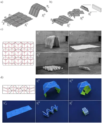
Figure 1.1 An example of a foldable origami structure with two, independent folded states. (a) A crease pattern and its resulting shelter configuration. (b) Miura-ori pattern and its folded configuration. (c) Overlay of the shelter pattern (black) and Miura-ori pattern (red) and the resulting structure folded into each configuration. (d) A thick panel equivalent of the shelter and Miura-ori foldable structure. (Image from Liu et. al21). ... 11

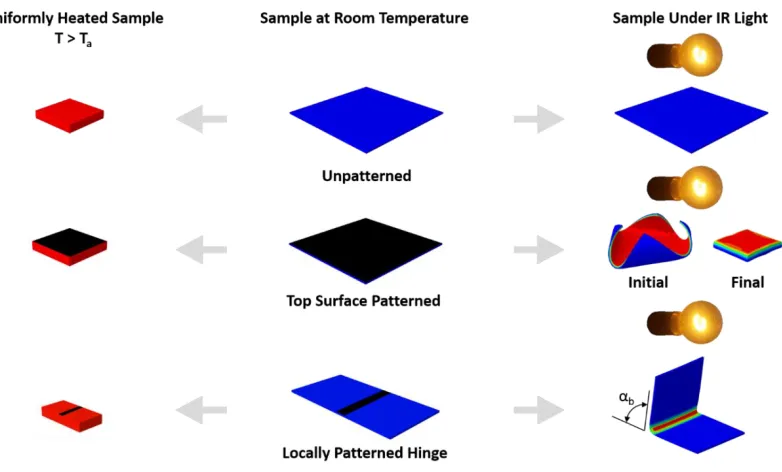
Figure 1.2 Response of ink patterned SMP sheets to uniform heating and exposure to IR light. Center column: patterned sheets do not shrink at room temperature. Left column: patterned sheets shrink uniformly when heated above the activation temperature Ta. Right column: and unpatterned sheet (top) does not absorb thermal energy from and IR light efficiently and does not heat above the activation temperature. Therefore, it does not shrink. A sheet coated in black ink (middle) will begin heating from the exposed surface. This generates a temperature and shrinkage gradient through the thickness, and the sheet initially curls towards toward the light before flattening out to shrink uniformly. A sheet patterned with discrete lines (bottom) will heat in the patterned region only. A gradient in temperature and shrinkage beneath the patterned region causes the sheet to fold along the line. ... 12

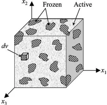
Figure 1.3 Illustration of the bi-phasic model used to predict the behavior of SMPs.30 Temperature converts frozen phases to active phases. The switch between frozen and active phases allows for the storage and release of entropic deformation. ... 13

Figure 2.1 Relative volume as a function of temperature (Image from Brinson and Brinson.3) ... 31

Figure 2.2 Creep and creep recovery tests: stress input (top) and qualitative material strain response (bottom). (Figure from Brinson and Brinson3). Strain has an immediate, elastic response upon stress application and removal and a time-dependent, viscous response after changes in stress. ... 31

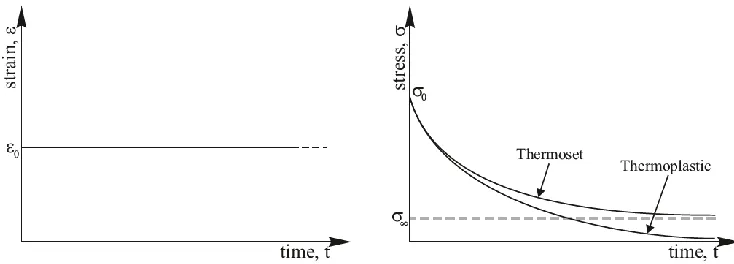
Figure 2.3 Stress relaxation test: strain input (left) and qualitative stress output (right). (Figure from Brinson and Brinson3) Stress has immediate elastic response followed by time-dependent, viscous response after initial strain application. Stress relaxes with time. ... 32

(16)

xii

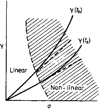
Figure 2.5 Isochronals taken at ta (see Figure 2.4) after the initiation of the creep experiment, γ(ta), and at tb, γ(tb). The diagram illustrates the transition from linear to non-linear viscoelastic behavior. Note that this is not the γ-σ plot that would be obtained in a conventional stress-strain test; the data are taken from creep experiments at different stresses.(Figure and caption from McCrum et

al.4_{) ... 33}

Figure 2.6 Maxwell model consisting of a spring and dashpot in series. ... 33

Figure 2.7 Kelvin-Voigt model consisting of a spring and dashpot in parallel... 33

Figure 2.8 Generalized Maxwell model ... 34

Figure 2.9 Generalized Kelvin-Voigt model. ... 34

Figure 2.10 Example master curve for a modified epoxy. (Original data from Cartner (1978).) Figure from Brinson and Brinson.3 ... 35

Figure 2.11 (A) Storage modulus, G', Loss Modulus, G", and (B) Phase angle, tan(δ) for a two-element generalized Maxwell model containing one free spring in parallel with a single Maxwell element (spring and dashpot in series). GR=0.01, G0=1, and τ=1. ... 35

Figure 2.12 Left: Relationship between strain, stress, and phase angle. Right: Depiction of phase angle in the complex plane. ... 36

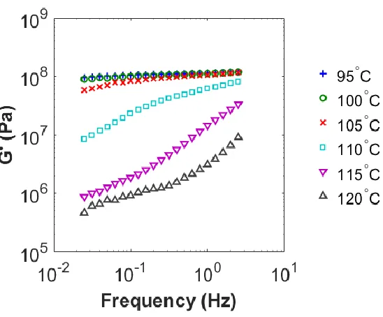
Figure 3.1 Storage modulus of PS as a function of temperature and frequency. ... 40

Figure 3.2 Viscoelastic Master Curve. Colors correspond to colors in Figure 3.1. Data for T < 105°C is approximately constant and therefore is omitted for clarity. Solid red line represents Prony series model fit. ... 40

Figure 3.3 Typical DSC results for polystyrene SMP. The dashed red line represents Tg=103°C. ... 41

(17)

xiii

Figure 3.5 Schematic of folding experimental setup. The sample rests on a hotplate pre-heated to 90°C. An IR light placed approximately 5 cm above the surface of the hotplate provides the external stimulus to initiate folding. ... 42

Figure 4.1 Illustration of shrinkage/folding behaviour of pre-strained Shrinky-Dinks SMP. Left column: samples acted on by uniform heating shrinks to approximately half the original size in each direction while increasing in thickness. Centre column: initial sample shape before heating. Shrinking or folding does not occur at room temperature. Right column: samples under radiant heating (e.g., by IR light) shrink in regions patterned with ink. Top row: unpatterned sample does not shrink. Middle row: entire top of sample coated with black ink initially curls before flattening and shrinking. Bottom row: locally patterned sample folds along hinge. ... 56

Figure 4.2 Folding model. (a) Mechanical boundary conditions during pre-straining sequence. (b) Mechanical and thermal boundary condition of folding model during recovery. (c) Folding model showing model symmetry and mesh. Labels specify the number of elements that span the indicated region. X1=20 elements for 1.0 and 1.2 mm hinge widths,.X1 = 19 elements for 1.5 and 2.0 mm hinge widths. X2 = 10 elements/mm of hinge width. Y = 22 elements. Z = 24 elements. ... 57

Figure 4.3 Illustration of thermal and mechanical boundary conditions for both in-plane recovery and folding models during pre-straining sequence. ... 58

Figure 4.4 Rheology data fit with Prony series model. (a) Experimental shear storage modulus (G’) data. (b) Shifted shear storage modulus data with Prony series model. (c) Experimental phase angle (tan δ) data. (d) Shifted phase angle data with Prony series model. Isothermal curves shifted using WLF equation (Supplemental Information Equation S4.2) with C1 = 17.44, C2 = 51.6, and Tref = 103°C. ... 59

Figure 4.5 Comparison of predicted values (lines) and experimental results (symbols) for in-plane shrinkage. (a) Isothermal recovery between 100 and 120°C, (b) Recovery for pre-strained samples heated uniformly at two heating rates. .... 60

Figure 4.6 Predicted folding results for 1 mm hinge width. (a) Modelled hinge surface heat flux (qin). (b) Comparison of averaged model and experimental hinge surface temperatures. (c) Comparison of model and experimental bending angles (αb). ... 61

(18)

xiv

(b) Predicted bending angle (αb) results for model (lines) and experimental (symbols) results. ... 62

Figure 4.8 Predicted variation of axial shrinkage and material thickness in the hinged region during folding for 1 mm hinge width. (a) Axial shrinkage at multiple times steps. (b) Axial shrinkage as a function of depth along folding angle bisection line. Note that the depth has been normalized by instantaneous hinge thickness. (c) Variation of hinge thickness along folding angle bisection line normalized by the pre-strained, unfolded thickness for duration of experiment. ... 63

Figure 4.9 Comparison of mass accumulation in hinged region for 2 mm hinge. (a) Experimental, early folding stages. (b) Experimental, late folding stages. (c) Computational model, shorter times. (d) Computational model longer times.64

Figure S4.1 Alternate geometric model that accounts for shrinkage of top and bottom hinge surfaces. (a) Geometric definitions. (b) Bending angle predicted by alternate geometric model for a range of top and bottom surface shrinkage values. .... 71

Figure S4.2 In-plane shrinkage model. (a) Mechanical boundary conditions during programming sequence. (b) Mechanical and thermal boundary condition of in-plane shrinkage model during shrinking process. (c) In-in-plane folding model showing model symmetry and mesh. Labels specify the number of elements that span the indicated region. X=10 elements. Y = 10 elements. Z = 4 elements. ... 72

Figure S4.3 Comparison of effect of short and long cooling times on isothermal recovery behavior. Samples programmed by short cooling time shown as solid lines. Samples programmed by long cooling time are shown as dashed lines. Experimental data shown as discrete points. ... 72

Figure S4.4 Bending angle results obtained by specifying experimentally measured hinge temperature for 1 mm hinge width model. Solid line represents model results. Symbols represent experimental results. ... 73

Figure S4.5 Constant IR flux results for 1 mm hinge. (a) Average hinge temperature results. (b) Bending angle results. Solid lines represent model results. Discrete points represent experimental results. ... 73

(19)

xv

across the hinge width). The hinge region is highlighted in red. (d) Thermal and mechanical loads applied during the folding sequence. (e) Plot of applied mechanical and thermal boundary conditions during pre-strain. (f) The viscoelastic master curve with a comparison of experimental results (discrete points) and the fit Prony series model (red line) at the glass transition temperature Tref=Tg=103°C. The blue discrete points are for the shear storage modulus, G', and the green discrete points are for the phase angle, tan(δ). .... 97

Figure 5.2 (a) Viscous heating caused a rapid rise in the average temperature on the mid-plane of model, perpendicular to the compression direction. (b) Temperature increases due to viscous heating affected the average stress on the mid-plane normal to the compression direction. (c) Relaxation of compressive normal stresses affected the average stress in the direction transverse to the compression direction on the mid-plane normal to the compression direction. (d) Transverse stresses along the plane parallel to the compression direction, after cooling, indicated significant differences in the residual stress state. The result in the top contour plot does not account for viscous heating, while the result in the bottom contour plot does. Contours are plotted on the undeformed mesh. ... 98

Figure 5.3 The viscous heat fraction and recovery temperature affected unconstrained recovery behavior. (a) Isothermal temperature Tsink=110°C. (b) Isothermal temperature Tsink=115°C. (c) Isothermal temperature Tsink=120°C. (d) Viscous heating during unconstrained recovery at 120°C caused an increase in internal temperature. The average temperature changes on the mid-plane due to conduction and viscous heating are plotted for Tsink=120°C. Viscous heat generation accounted for ~5.3% of the total temperature increase. ... 99

Figure 5.4 Viscous heating occurred during variations on the original pre-straining sequence. (a) Viscous heating caused a rise in temperature during the compression step for all pre-strain variations considered. A common time scale is used for all pre-strain variations considered. (b) Due to viscous stress relaxation during pre-strain, the unconstrained recovery response of models exposed to a Tsink=110°C convective boundary condition were approximately identical. ... 100

(20)

xvi

Figure 5.6 Demonstration of folding and unfolding of a single-hinged SMP sheet. (a) The material was first pre-strained according to the pre-strain sequence. (b) The sheet folded in response to a specified surface heat flux in the hinged region. (c) The folded shape was retained after removing the heat flux and cooling the material to below Tg. (d) The sheet unfolded and shrank after application of a uniform, isothermal boundary condition with a temperature greater than Tg. ... 102

Figure 5.7 Results for the investigation of the effects of sheet thickness on bending angle, αb, using a constant surface heat flux applied to the hinge region. (a) Plot of αb as a function of time for multiple sheet thicknesses. All sheets had the same initial, transverse pre-strain. (b) A comparison of the maximum bending angle,

αb,max, and time to reach αb,max for each sheet thickness. (c) Images of the folded

models at αb,max. Color indicates temperature from blue (cool) to red (hot). 103

Figure 5.8 Results for the investigation of the effects of hinge width on bending angle, αb. (a) αb plotted as a function of time for a range of hinge widths. (b) A comparison of the maximum bending angle, αb,max, and time to reach αb,max. (c) Images of folded model at αb,max. Color indicates temperature from blue (cool) to red (hot). ... 104

Figure 5.9 Results for the investigation of the effects of the degree of pre-strain on bending angle, αb. (a) αb as a function of time for a range of pre-strains listed by maximum possible shrinkage upon recovery. (b) Maximum bending angle,

αb,max, and time to reach αb,max. (c) Images of folded model at αb,max for each

degree of pre-strain. Color indicates temperature from blue (cool) to red (hot). ... 105

Figure 5.10 Bending results from a specified temperature boundary condition applied to a 1 mm wide hinged region. (a) Bending angle, αb, and the rate of folding was affected by the applied hinge temperature. (b) Contour plots indicate a gradient in temperature. Unfolding occurred when a sufficiently high temperature was attained on the back surface of the hinge. ... 106

(21)

xvii

image: Valley folds with a gradient of spacing cause the sheet to curve in a discontinuous fashion due to the direct curvature mechanism. The scale bars are 25 mm. ... 126

Figure 6.2 Progression of deformation of SMP samples 50% covered with black ink. Images progress in sequence of time from top to bottom. Both synclastic and anticlastic samples take less than 10 seconds to complete their activation response. Left two columns: Samples patterned with black strips along the outer edges bent up initially along the edges before the sample was curled towards the inked side in a synclastic (positive Gaussian curvature) manner. Right two columns: Samples patterned with a black strip along the middle initially folded along the ink pattern then curled away from the ink in an anticlastic (negative Gaussian curvature) manner. The colors in the computational images represent temperatures ranging from below Tg (blue) to above Tg (red). Intermediate temperatures are depicted in green. The scale bar is 5 mm. ... 127

Figure 6.3 Changes to the ink darkness resulted in a transition from a synclastic to anticlastic response. The percent ink darkness of each strip was superimposed on the patterns in the left column. (A, B) Synclastic, positive Gaussian curvature. (C) Random curvature formed by uniform ink coverage. (D, E) Anticlastic, negative Gaussian curvature. Slight heating of the previously uninked strips in (D) softened the material enough that the experimentally seen anticlastic behavior was predicted computationally. The colors in the computational images represent temperatures ranging from below Tg (blue) to above Tg (red). The scale bar is 5 mm. ... 128

Figure 6.4 An illustration of the effects of changes to the substrate aspect ratio while maintaining 50% ink coverage. (A) Two equal-with horizontal strips produced a synclastic response. (B) A single, centrally located, horizontal strip produced an anticlastic response. (C) A horizontal strip moved to the edge resulted in a “U” shape. (D) An equal width border created a similar synclastic response as in (A). In general, the total deformation was influenced by the substrate aspect ratio. The colors in the computational images represent temperatures ranging from below Tg (blue) to above Tg (red). Scale bars are 5 mm. ... 129

(22)

xviii

convenience. Scale bars are 5 mm for samples A-C and 10 mm for samples D-E. ... 130

Figure 6.6 Comparison of experimentally and computationally generated structures utilizing both direct and indirect mechanisms. (A) Spatially varying curvature was controlled by ink distribution. There was excellent visual agreement between the computational and experimental results. The colors in the computational images represent temperatures ranging from below Tg (blue) to above Tg (red). (B-C) 3D point clouds produced via serial sectioning for both the bordered and gradient ink patterns, B and C respectively. The black points represent the computational results, and the colored points indicate the experimental samples. Individual panels are extracted on the right-hand columns to clarify the excellent agreement between the experimental and computational results. The scale bars are 5 mm. ... 131

Figure 6.7 Quantitative comparison of the computationally and experimentally generated structures. (A) The computational result for the gradient sample is shown with a representative radius of curvature (Rc) and dihedral angle (θ) for clarification. The radius of curvature was calculated using three points along the curve of the panel. The colors in the computational images represent temperatures ranging from below Tg (blue) to above Tg (red). (B) The dihedral angle values, θ, are plotted for both structures seen in Figure 6.6. (C) The radius of curvature values, Rc, are plotted for both structures seen in Figure 6.6. There is excellent agreement between the experimental and computational results. The scale bar is 5 mm. ... 132

Figure 6.8 The four-paneled bio-inspired structures were extended to a greater number of panels with similar behavior, allowing for a wider range of applications. (A) A hexagonally-based, six-paneled array was applied as a small gripping device. (B) Grippers based on these designs were able to encompass and hold small objects, such as the head of a bolt. (C) Due to their global curvature and lightweight nature, these grippers were able to firmly grip the bolt and could easily hold ~925x their own weight. The scale bars are 10 mm. ... 133

(23)

xix

Figure S6.2 A graphical and visual depiction of how surface temperature and normalized IR absorption increases with nominal and actual ink density for experimental (A) and computational (B) results. The temperature values used within the graph are directly correlated to the values on the thermal image (A). The dashed black lines overlaid on the IR image visually depict that the surface temperature values were recorded at the centerline (squares) and lower edge (circles). The lower image in B represents the ink pattern where the grey regions are unpatterned and the black regions indicate ink coverage. ... 138

Figure S6.3 An illustration of the effects of changes to the sample aspect ratio while maintaining the designated gradient pattern. Samples became more curved with the increase in aspect ratio, while the same general trend was observed for each gradient ink pattern. The scale bar is 5 mm for 3:1 aspect ratio samples and 10 mm for the 2:1 and 1:1 aspect ratio samples... 139

Figure S6.4 Serial section process used to obtain the digital, 3D point cloud of the bio-inspired structures. (A) The samples were painted, casted, milled in ~ 0.5 mm segments, and digitally imaged to acquire the necessary data points. The final point cloud can be seen for both the (B) indirect and (C) direct mechanism of curvature. The gradient in color corresponds to changes in height while the black data points represent the computational results. ... 140

Figure S6.5 Schematic defining variables in Equations S6.1-S6.4 ... 140

Figure 7.1 (A) Hinged folding can be used to produce 3D structures of intermediate complexity from initially flat sheets. The orientation and spacing of hinges, as well as the hinge width and substrate geometry affects the final shape and bending angle of the sheet. (B) Self-folding in our thermally activated SMP sheet arises from the viscoelastic material behavior as the local temperature traverses the glass transition temperature, Tg = 103°C. A Prony series with six terms is used to represent the viscoelastic master curve. (C) Representative thermal and mechanical boundary conditions are applied to the sheet to pre-strain the material and subsequently induce the folding response. ... 158

Figure 7.2 (A) The incident heat flux

q



incauses a similar increase in the average hinge

(24)

xx

vectors p1 and p2 indicates that each hinge angle θ produces the same folding motion. This is the view shown in the lower right corner of Figure 7.1B. ... 159

Figure 7.3 The constrained bending reaction force is evaluated for 1.0, 1.5, and 2.0 mm hinge widths. (A) Increasing the hinge width results in a slight temperature increase. (B) Increasing the hinge width increases the maximum total reaction force while decreasing the time to this maximum force. (C) The reaction force is dominated by the force due to axial shrinking in the hinge region. (D) Prior to 1 second, the hinge bends backwards due to thermal expansion and creates a positive reaction force. At approximately 1 second, material shrinking becomes activated which results in a negative reaction force. Decreasing the hinge width results in a vertical reaction force with a larger magnitude that occurs at a later time than for wider hinges. ... 160

Figure 7.4 Placing two parallel hinges in close proximity to each other increases the bending angle. For instance, two 1 mm hinges placed in close proximity exceeds the maximum bending angle, αb,max, of a single 2 mm hinge width pattern. The spacing between the two hinges affects the maximum bending angle and the time to fold as seen for the 1 mm hinge width results. For the 2 mm hinge width results, the transient bending angle is approximately the same for the three spacings, ΔW, considered. The red x at t=1.35 s indicates the last time step before the folding faces of the model intersect. ... 161

Figure 7.5 Contour plots of the temperature distribution in the cross-section of the hinge show how transverse conduction creates a wider effective hinge width. (A) The space between the 1 mm hinges becomes activated due to conduction. (B) The material between the 2 mm hinges does not sufficiently heat to become activated due in part to the faster response time of this pattern. ... 162

Figure 7.6 Self-folding responses from three initial temperatures, 30, 60, and 90°C, are considered. (A) Lower initial temperatures result in a delay in the time it takes for the average hinge temperature to exceed the glass transition temperature. (B) Decreasing the initial temperature delays and broadens the peak bending angle. ... 162

Figure 7.7 (A) Increasing the incident heat flux results in a faster heating rate as indicated by the average hinge temperature. (B) The increased heating rate results in a faster folding rate and higher maximum bending angle. ... 163

(25)

xxi

reaction force is dominated by the axial contraction force regardless of surface heat flux. ... 164

Figure 7.9 The effect of changing the width of the hinge is evaluated for widths of (A) 0.5 mm, (B) 1 mm, (C) 2.5 mm, (D) 5 mm, (E) 7.5 mm, (F) 9 mm, and (G) 9.5 mm. The width of the substrate is 10 mm. The material response transitions from hinged folding to smooth curvature between 1 and 2.5 mm. The inset images show the cross-section of the sample. ... 165

Figure 7.10 The patterns from Figure 7.9 are inverted so that the center stripe is unpatterned, but the outer panels are coated in black ink. The unpatterned center stripe has a width of (A) 0.5 mm, (B) 1 mm, (C) 2.5 mm, (D) 5 mm, (E) 7.5 mm, (F) 9 mm, and (G) 9.5 mm. Above 5 mm, the patterned region is not large enough to induce significant curvature in the unpattered region. ... 166

Figure 7.11 Axisymmetric gradients on 1-inch diameter discs Top row: a gradient of ink that increases in the radial direction caused the sheet to form a bowl. Bottom row: a gradient of ink that decreases in the radial direction causes the sheet to buckle into a saddle shape. ... 167

Figure 7.12 A solid outer ring pattern causes the sheet to curl into a bowl-like shape when exposed to an IR light. The size of the wrinkles around the perimeter can be controlled by the width of the pattern. Top row: outer ring width is 25% of the disc radius. Middle row: outer ring width is 50% of the disc radius. Bottom row: outer ring width is 75% of the disc radius. ... 168

Figure 7.13 A solid inner ring pattern causes the sheet to buckle into a saddle shape when exposed to an IR light. The magnitude of the out of plane deformation can be controlled by the width of the pattern. Top row: outer ring width is 25% of the disc radius. Middle row: outer ring width is 50% of the disc radius. Bottom row: outer ring width is 75% of the disc radius. ... 169

Figure 7.14 A concentric ring pattern with the ring centered at 50% of the radius. The width of the ring increases from 12.5% of the radius (top row), to 25% (middle row), and 50% (bottom row). ... 170

Figure 7.15 A concentric ring pattern with the unpatterned ring centered at 50% of the radius. The width of the unpatterned ring decreases from 50% of the radius (top row), to 25% (middle row), and 12.5% (bottom row). ... 171

Figure 7.16 Gradient wedges generated by a sinusoidal wave. Top Row: 4 patterned wedges. Bottom Row: 8 patterned wedges. ... 172

(26)

1

Chapter 1: Introduction

1.1 Overview

Consider what it takes to manufacture and put into use an everyday object, such as a chair. This process begins with manufacturing steps that require time consuming and costly operations to produce components of the chair. These steps may be additive or subtractive in nature, i.e., material is added to or removed from the workpiece, to produce individual parts and assemblies. These manufacturing steps bring the chair to its near final, three-dimensional (3D) shape. The chair is then shipped in this bulky state to its final destination. This results in empty space during shipping, which reduces the number of chairs that can be transported. Upon reaching the final destination, some assembly may be required before using the chair.

Alternatively, folding systems allow the use of high throughput patterning and cutting techniques to produce a two-dimensional (2D) representation of the chair. The chair ships in its flat state to the final destination where it is put into use through folding and unfolding manipulations. The incorporation of active materials into a folding structure results in a self-folding structure that responds to the environment. Active materials change shape or have significantly altered properties in response to external stimuli such as heat, light, or solvents.

1.1.1 Engineered Origami and Kirigami

(27)

2

closely related approach, kirigami, incorporates cuts into the material and can be used to develop more complex structures.6–11

A primary thrust of origami engineering is the development of fold patterns and the associated kinematics of folding and unfolding. Commonly utilized fold patterns include the waterbomb12,13 base and Miura-ori.8,14–17 Other crease patterns can be designed using models that typically assume that the material has a negligible thickness and that the material forms a sharp, zeroth-order fold at the crease line. The use of finite thickness materials invalidates this assumption, which has led to the development of models for smooth folds18 and folding of structures with finite thicknesses.19,20 Further, origami patterns can be superimposed to obtain functional structures with multiple stable states, as seen in Figure 1.1.21 Kirigami structures have been developed for beam steering and solar tracking applications.7,10 In these systems, linear actuation produces significant changes in the orientation of facets on the structure. Another advantage of self-folding origami is that it allows full access to the surface of the material for patterning at the microscale, and the active materials in the structure can be used to control shape at the macroscale.22 Self-folding can also be actuated by relaxation of mechanical loads. For instance, release of mechanical pre-strain in an elastomeric substrate can cause rigid origami structures to pop-up from a flat state.2,23,24

1.1.2 Self-Folding Origami

(28)

3

methods for patterning and cutting sheets, (iii) facile or autonomous assembly of 3D structures reduces time and cost of deploying the product. Converting a planar sheet into a 3D shape requires deformation of the sheet, which can be achieved by physical manipulation or by using active materials, i.e., materials that can change shape (i.e., shrink or expand) in response to an external stimulus such as light, heat, or solvent.28–41 Conventionally, these responsive materials are placed in regions where deformation is desired.30,31,39,41–43 Self-folding can be used to obtain 3D structures for an array of applications, including medical stents,44–46_antennas,47_and engineered origami applications, such as space telescopes.48 Self-folding can be attained through the use of active materials, such as hydrogels,49–53 shape memory alloys (SMAs),54–56 or shape memory polymers (SMPs),30,42,57–59 or either alone or in combination with passive materials including wood, paper, or polymers.

Hydrogels are active materials that swell in response to exposure to solvents,12,13,33,42,57,59–66 and therefore represent suitable candidates for inducing changes in curvature in initially flat sheets. Bilayers of hydrogels28,32,38,51,67–70 or hydrogels patterned with stiff regions37,53,71 can produce curved 3D structures due to differential swelling. However, hydrogel based materials generally possess a slow response time, low moduli, and require continuous solvent exposure to maintain their deformed shape.

(29)

4

response and range of activation temperatures, but they are generally more expensive and often must be used in combination with a second material.

Conventional SMPs are attractive shape changing alternatives to gels and SMAs due to their relatively short response time, low cost, high stiffness, and potential responsiveness to a wide range of activation stimuli. Activation stimuli for SMPs include heat, light, and electric fields.58,73 Heat activated SMPs can respond to a variety of heat sources, such as uniform heating,31,63,74_{local energy absorption,}14,30,41,43,75_{or Joule heating.}42,61_{SMPs can generate} discretely folded structures in laminated composites42,60–63 or homogeneous sheets.30,31,37,41 Additionally, heat activated SMPs maintain their shape upon removal of the stimulus.

Of these active materials, SMPs are attractive due to their low cost, ease of processing, ability to recover large deformation, and a diverse selection of activation stimuli, i.e., heat,30,42,60,61,63,76_light,77–79_pH,80_solvents,49,81–83_{and magnetic fields.}84 _{Based on} these advantages, I sought an approach to obtain 3D objects from thermoplastic SMP sheets by using localized material shrinking. Although SMPs have many applications, I am primarily interested in using the material as thermally responsive actuators for self-folding origami structures73,85,86 because of the potential multifunctional applications.

1.1.3 Experimental Studies

The typical thermo-mechanical cycle applied to heat activated SMPs87–89 involves straining the polymer, which is initially at an elevated temperature near the glass transition temperature (Tg), to some temporary shape (e.g., an elongated sheet). After cooling, the

(30)

5

through a viscoelastic strain recovery process, referred to as shrinkage. Shrinkage is a function of both time and temperature and occurs more rapidly at higher temperatures.90

I have shown that black ink patterned on SMPs can locally absorb light to induce folding.30,90,91 In this investigation, I utilized pre-strained polystyrene SMP sheets in the form of commercially available Grafix® shrink film. These amorphous, biaxially pre-strained polystyrene sheets shrink in-plane to approximately half of the original dimensions when thermally activated (the activation temperature, Ta, is approximately

the same as Tg, Tg = 103°C). Figure 1.2 outlines schematically the behavior of three

SMP samples when exposed to two different heat sources. The center column depicts the samples before heating. All three configurations shrink uniformly when heated above Ta as shown in the left column of Figure 1.2. These configurations behave

differently when exposed to a radiant heat source, e.g., infrared (IR) light. A transparent SMP does not shrink readily when exposed to the radiant heat source because the polymer does not absorb the radiant thermal energy efficiently (Figure 1.2, top row).90 Samples coated with black ink absorb light more efficiently than uncoated samples and a temperature gradient develops through the thickness of the sheet. Thus, the polymer shrinks locally wherever the temperature reaches Ta. This temperature gradient results

(31)

6

gradient, and the polymer folds along the ink pattern (Figure 1.2, bottom row).30 While folding, the un-patterned regions do not shrink noticeably. Other approaches to induce self-folding in thermally activated SMP sheets include the use of uniform1 or Joule heating42,63 in SMP composites, or using microwaves76 or lasers.91 Previously, a simple geometrical model was developed and presented that predicts the maximum and transient bending angles, αb (defined graphically in the lower right image of Figure 1.2)

of self-folding polymer sheets.90_{However, that geometrical model does not provide} fundamental thermo-mechanical understanding of the relevant material mechanisms and requires experimentally measured temperatures to predict transient αb. In addition

to the hinged folding behavior, a balance of internal stresses that arise from material shrinkage can be used to induce curvature in the polymer sheet. In our system, the recovery rate can be controlled by the rate of localized energy absorption and the subsequent heat dissipation of the patterned region. This can be realized by changing the intensity of the IR light source or the light absorptivity of the ink.43 Complex 3D structures can be obtained by combining multi-hinged patterns with cuts in the material.41

As part of this investigation, I investigated viscous heating during the shrinking and folding of SMP sheets. Viscous heat generation arises from viscous sliding and shearing of polymer chains at the molecular level.92–96 This heating effect is significant in many polymer systems during the transition from glassy to rubbery behavior, and is prevalent near Tg. Viscous

(32)

7

cyclic mechanical loading.98,99 In these materials, viscous heating can lead to significant thermal increases,98_{which affect the behavior of the damper. Hence, the effects of viscous} heating must be understood among a myriad of effects, such as damping and material failure.

1.1.4 Computational Studies

(33)

8

have investigated the effects of the thermal and mechanical history applied to the polymer on the recovery behavior89,102_{and finite deformation viscoelasticity}101,109,115–119 using a combination of finite element or numerical analysis and experimental evaluations.

1.2 General Research Objectives and Approach

The objective of this research is to model computationally the behavior of SMPs used for self-folding origami. Self-folding is affected significantly by the heat absorption and heat transfer, the non-linear relationship between temperature and shrinkage, and the conservation of mass in the material. Therefore, in this investigation, I use a 3D, non-linear, finite element framework with a thermo-viscoelastic material model and fully-coupled thermo-mechanical solution to gain insights into the fundamental behavior of folding SMP sheets that cannot be obtained experimentally. To this end, I systematically investigate the effects of hinge orientation, size, and spacing, as well as the effects of initial temperature and surface heat flux. Further, this computational framework provides an understanding of the sensitivity of folding to the surface heat flux and sample pre-straining process.

(34)

9

manually. An alternative method is to induce changes in material dimensions, such as through strain that arises from swelling or shrinking of SMP sheets. I explored two strategies, termed the ‘direct’ and ‘indirect’ mechanism of curvature to convert planar thermoplastic sheets into

3D shapes. The direct mechanism, achieves curvature by applying strain directly to the portions of the sheet to be curved. For the indirect mechanism, curvature can arise ‘indirectly’ in

response to internal stresses induced by one region shrinking relative to adjacent regions. Within the framework of the computational model, I sought a better understanding of the thermo-mechanical mechanisms that lead to shrinking and folding in SMP sheets. These mechanisms include time and temperature dependent moduli, viscoelastic recovery, external temperature fields, surface heat fluxes, internal dissipative viscous heat generation, and diffusive heat conduction. Viscous heating occurs whenever there is viscous sliding among polymer chains, i.e., during both the initial straining and subsequent relaxing of SMPs. Given the relationship between temperature and the shrinking or folding of SMP sheets, viscous heating, in combination with other heating mechanisms, would affect the shape change response of the material. Additionally, viscous heating during shape recovery causes an increase in temperatures that significantly affect the strain relaxation rate.

(35)

10

diffuses heat that arises from internal and external sources. Heating affects instantaneous moduli, which are related to TTSP, and also affects thermal expansion, which is related to thermal stresses and strains. All these thermal components affect the internal temperature distribution, but they are also coupled to the stresses through viscous heating. In addition to the imposed thermal loading, each thermal component affects thermo-mechanistic aspects of shrinking and folding, which can provide further understanding regarding how time, temperature, and stresses affect material response.

1.3 Dissertation Organization

(36)

11

(37)

12

Figure 1.2 Response of ink patterned SMP sheets to uniform heating and exposure to IR light. Center column: patterned sheets do not shrink at room temperature. Left column: patterned sheets shrink uniformly when heated above the activation temperature Ta. Right column: and unpatterned sheet (top) does not absorb thermal energy

(38)

13

Figure 1.3 Illustration of the bi-phasic model used to predict the behavior of SMPs.30_{Temperature converts frozen}

(39)

14

References

1 J.-H. Na, A. A. Evans, J. Bae, M. C. Chiappelli, C. D. Santangelo, R. J. Lang, T. C. Hull and R. C. Hayward, Adv. Mater., 2015, 27, 79–85.

2 Z. Yan, F. Zhang, J. Wang, F. Liu, X. Guo, K. Nan, Q. Lin, M. Gao, D. Xiao, Y. Shi, Y. Qiu, H. Luan, J. H. Kim, Y. Wang, H. Luo, M. Han, Y. Huang, Y. Zhang and J. A. Rogers, Adv. Funct. Mater., 2016, 26, 2629–2639.

3 G. Stoychev, N. Puretskiy and L. Ionov, Soft Matter, 2011, 7, 3277–3279. 4 A. Lebée, Int. J. Space Struct., 2015, 30, 55–74.

5 C. Qiu, V. Aminzadeh and J. S. Dai, J. Mech. Des., 2013, 135, 111004–111004. 6 Q. Zhang, J. Wommer, C. O’Rourke, J. Teitelman, Y. Tang, J. Robison, G. Lin and J.

Yin, Extreme Mech. Lett., 2017, 11, 111–120.

7 A. Lamoureux, K. Lee, M. Shlian, S. R. Forrest and M. Shtein, Nat. Commun., 2015,

6.

8 C. Jianguo, D. Xiaowei and F. Jian, Smart Mater. Struct., 2014, 23, 94011.

9 Y. Tang, G. Lin, S. Yang, Y. K. Yi, R. D. Kamien and J. Yin, Adv. Mater., 2016, n/a-n/a.

10 W. Wang, C. Li, H. Rodrigue, F. Yuan, M.-W. Han, M. Cho and S.-H. Ahn, Adv. Funct. Mater., 2017, n/a-n/a.

11 S. Yang, I.-S. Choi and R. D. Kamien, MRS Bull., 2016, 41, 130–138.

12 B. H. Hanna, J. M. Lund, R. J. Lang, S. P. Magleby and L. L. Howell, Smart Mater. Struct., 2014, 23, 94009.

13 B. H. Hanna, S. P. Magleby, R. J. Lang and L. L. Howell, J. Appl. Mech., 2015, 82, 081001–081001.

14 K. Suzuki, H. Yamada, H. Miura and H. Takanobu, Microsyst. Technol., 2007, 13, 1047–1053.

(40)

15

17 K. C. Cheung, T. Tachi, S. Calisch and K. Miura, Smart Mater. Struct., 2014, 23, 94012.

18 E. A. Peraza Hernandez, D. J. Hartl and D. C. Lagoudas, J. Mech. Robot., 2016, 8, 61019-61019–22.

19 Y. Chen, R. Peng and Z. You, Science, 2015, 349, 396–400.

20 M. R. Morgan, R. J. Lang, S. P. Magleby and L. L. Howell, Mech. Sci., 2016, 7, 69– 77.

21 X. Liu, J. M. Gattas and Y. Chen, Sci. Rep., 2016, 6, 36883.

22 S. Janbaz, R. Hedayati and A. A. Zadpoor, Mater. Horiz., 2016, 3, 536–547.

23 S. Xu, Z. Yan, K.-I. Jang, W. Huang, H. Fu, J. Kim, Z. Wei, M. Flavin, J. McCracken, R. Wang, A. Badea, Y. Liu, D. Xiao, G. Zhou, J. Lee, H. U. Chung, H. Cheng, W. Ren, A. Banks, X. Li, U. Paik, R. G. Nuzzo, Y. Huang, Y. Zhang and J. A. Rogers, Science, 2015, 347, 154–159.

24 Z. Yan, F. Zhang, F. Liu, M. Han, D. Ou, Y. Liu, Q. Lin, X. Guo, H. Fu, Z. Xie, M. Gao, Y. Huang, J. Kim, Y. Qiu, K. Nan, J. Kim, P. Gutruf, H. Luo, A. Zhao, K.-C. Hwang, Y. Huang, Y. Zhang and J. A. Rogers, Sci. Adv., 2016, 2, e1601014.

25 D. H. Gracias, Curr. Opin. Chem. Eng., 2013, 2, 112–119.

26 E. A. Peraza-Hernandez, D. J. Hartl, R. J. Malak Jr and D. C. Lagoudas, Smart Mater. Struct., 2014, 23, 94001.

27 L. Ionov, Polym. Rev., 2013, 53, 92–107.

28 J. C. Athas, C. P. Nguyen, B. C. Zarket, A. Gargava, Z. Nie and S. R. Raghavan, ACS Appl. Mater. Interfaces, 2016, 8, 19066–19074.

29 H. Arazoe, D. Miyajima, K. Akaike, F. Araoka, E. Sato, T. Hikima, M. Kawamoto and T. Aida, Nat. Mater., 2016, 15, 1084–1089.

30 Y. Liu, J. K. Boyles, J. Genzer and M. D. Dickey, Soft Matter, 2012, 8, 1764–1769. 31 D. Davis, B. Chen, M. D. Dickey and J. Genzer, J. Mech. Robot., 2016, 8, 031014–

031014.

(41)

16

34 Q. Guo, A. K. Mehta, M. A. Grover, W. Chen, D. G. Lynn and Z. Chen, Appl. Phys. Lett., 2014, 104, 211901.

35 A. I. Egunov, J. G. Korvink and V. A. Luchnikov, Soft Matter, 2015, 12, 45–52. 36 D. J. Glugla, M. D. Alim, K. D. Byars, D. P. Nair, C. N. Bowman, K. K. Maute and R.

R. McLeod, ACS Appl. Mater. Interfaces, 2016, 8, 29658–29667.

37 J. Kim, J. A. Hanna, M. Byun, C. D. Santangelo and R. C. Hayward, Science, 2012,

335, 1201–1205.

38 J. Ma, X. Mu, C. N. Bowman, Y. Sun, M. L. Dunn, H. J. Qi and D. Fang, J. Mech. Phys. Solids, 2014, 70, 84–103.

39 R. Takahashi, Y. Ikura, D. R. King, T. Nonoyama, T. Nakajima, T. Kurokawa, H. Kuroda, Y. Tonegawa and J. P. Gong, Soft Matter, 2016, 12, 5081–5088.

40 J. J. Wie, K. M. Lee, M. L. Smith, R. A. Vaia and T. J. White, Soft Matter, 2013, 9, 9303–9310.

41 Q. Zhang, J. Wommer, C. O’Rourke, J. Teitelman, Y. Tang, J. Robison, G. Lin and J. Yin, Extreme Mech. Lett., Article in Press.

42 S. M. Felton, M. T. Tolley, B. Shin, C. D. Onal, E. D. Demaine, D. Rus and R. J. Wood,

Soft Matter, 2013, 9, 7688–7694.

43 Y. Lee, H. Lee, T. Hwang, J.-G. Lee and M. Cho, Sci. Rep., 2015, 5, 16544.

44 G. M. Baer, W. Small, T. S. Wilson, W. J. Benett, D. L. Matthews, J. Hartman and D. J. Maitland, Biomed. Eng. OnLine, 2007, 6, 43.

45 S. Reese, M. Böl and D. Christ, Comput. Methods Appl. Mech. Eng., 2010, 199, 1276– 1286.

46 L. Xue, S. Dai and Z. Li, J. Mater. Chem., 2012, 22, 7403–7411.

47 G. J. Hayes, Y. Liu, J. Genzer, G. Lazzi and M. D. Dickey, IEEE Trans. Antennas Propag., 2014, 62, 5416–5419.

48 J. T. Early, R. Hyde and R. L. Baron, 2004, vol. 5166, pp. 148–156.

(42)

17

50 S.-H. Kim, H. R. Lee, S. J. Yu, M.-E. Han, D. Y. Lee, S. Y. Kim, H.-J. Ahn, M.-J. Han, T.-I. Lee, T.-S. Kim, S. K. Kwon, S. G. Im and N. S. Hwang, Proc. Natl. Acad. Sci., 2015, 201504745.

51 C. Yoon, R. Xiao, J. Park, J. Cha, T. D. Nguyen and D. H. Gracias, Smart Mater. Struct., 2014, 23, 94008.

52 Y. Zhang and L. Ionov, Langmuir, 2015, 31, 4552–4557.

53 E. Palleau, D. Morales, M. D. Dickey and O. D. Velev, Nat. Commun., 2013, 4, 2257. 54 E. A. Peraza-Hernandez, D. J. Hartl and R. J. M. Jr, Smart Mater. Struct., 2013, 22,

94008.

55 C. Lelieveld, K. Jansen and P. Teuffel, J. Intell. Mater. Syst. Struct., 2016, 27, 2038– 2048.

56 M. Taya, Y. Liang, O. C. Namli, H. Tamagawa and T. Howie, Smart Mater. Struct., 2013, 22, 105003.

57 L. Ionov, Soft Matter, 2011, 7, 6786.

58 J. Leng, X. Lan, Y. Liu and S. Du, Prog. Mater. Sci., 2011, 56, 1077–1135.

59 E. Hawkes, B. An, N. M. Benbernou, H. Tanaka, S. Kim, E. D. Demaine, D. Rus and R. J. Wood, Proc. Natl. Acad. Sci. U. S. A., 2010, 107, 12441–5.

60 S. Felton, M. Tolley, E. Demaine, D. Rus and R. Wood, Science, 2014, 345, 644–646. 61 S. M. Felton, K. P. Becker, D. M. Aukes and R. J. Wood, J. Micromechanics

Microengineering, 2015, 25, 85004.

62 S. Miyashita, L. Meeker, M. T. Tolley, R. J. Wood and D. Rus, Smart Mater. Struct., 2014, 23, 94005.

63 M. T. Tolley, S. M. Felton, S. Miyashita, D. Aukes, D. Rus and R. J. Wood, Smart Mater. Struct., 2014, 23, 94006.

64 S. Daynes, R. S. Trask and P. M. Weaver, Smart Mater. Struct., 2014, 23, 125011. 65 E. T. Filipov, T. Tachi and G. H. Paulino, Proc. Natl. Acad. Sci., 2015, 201509465. 66 D. Hartl, D. Lagoudas, R. Malak, M. Frecker and Z. Ounaies, Smart Mater. Struct.,

(43)

18

67 D. Morales, E. Palleau, M. D. Dickey and O. D. Velev, Soft Matter, 2014, 10, 1337– 1348.

68 G. Stoychev, S. Turcaud, J. W. C. Dunlop and L. Ionov, Adv. Funct. Mater., 2013, 23, 2295–2300.

69 H. Thérien-Aubin, Z. L. Wu, Z. Nie and E. Kumacheva, J. Am. Chem. Soc., 2013, 135, 4834–4839.

70 R. Vaia and J. Baur, Science, 2008, 319, 420–421.

71 Z. L. Wu, M. Moshe, J. Greener, H. Therien-Aubin, Z. Nie, E. Sharon and E. Kumacheva, Nat. Commun., 2013, 4, 1586.

72 E. A. Peraza-Hernandez, D. J. Hartl and R. J. M. Jr, Smart Mater. Struct., 2013, 22, 94008.

73 Y. Liu, J. Genzer and M. D. Dickey, Prog. Polym. Sci., 2016, 52, 79–106.

74 B. An, S. Miyashita, M. T. Tolley, D. M. Aukes, L. Meeker, E. D. Demaine, M. L. Demaine, R. J. Wood and D. Rus, in 2014 IEEE International Conference on Robotics and Automation (ICRA), 2014, pp. 1466–1473.

75 K. N. Long, T. F. Scott, H. Jerry Qi, C. N. Bowman and M. L. Dunn, J. Mech. Phys. Solids, 2009, 57, 1103–1121.

76 D. Davis, R. Mailen, J. Genzer and M. Dickey, RSC Adv., 2015, 89254–89261. 77 J. S. Sodhi, P. R. Cruz and I. J. Rao, Int. J. Eng. Sci., 2015, 89, 1–17.

78 R. V. Beblo and L. M. Weiland, J. Appl. Mech., 2008, 76, 11008. 79 R. V. Beblo and L. M. Weiland, J. Appl. Mech., 2011, 78, 61016.

80 X.-J. Han, Z.-Q. Dong, M.-M. Fan, Y. Liu, J.-H. Li, Y.-F. Wang, Q.-J. Yuan, B.-J. Li and S. Zhang, Macromol. Rapid Commun., 2012, 33, 1055–1060.

81 D. Morales, I. Podolsky, R. W. Mailen, T. Shay, M. D. Dickey and O. D. Velev,

Micromachines, 2016, 7, 98.

82 C. Yoon, R. Xiao, J. Park, J. Cha, T. D. Nguyen and D. H. Gracias, Smart Mater. Struct., 2014, 23, 94008.

(44)

19

84 P. R. Buckley, G. H. Mckinley, T. S. Wilson, W. Small, W. J. Benett, J. P. Bearinger, M. W. Mcelfresh and D. J. Maitland, IEEE Trans. Biomed. Eng., 2006, 53, 2075–2083. 85 K. Oliver, A. Seddon and R. S. Trask, J. Mater. Sci., 2016, 1–27.

86 J. Leng, X. Lan, Y. Liu and S. Du, Prog. Mater. Sci., 2011, 56, 1077–1135. 87 X. Chen and T. D. Nguyen, Mech. Mater., 2011, 43, 127–138.

88 M. Behl and A. Lendlein, Mater. Today, 2007, 10, 20–28.

89 F. Castro, K. K. Westbrook, K. N. Long, R. Shandas and H. J. Qi, Mech. Time-Depend. Mater., 2010, 14, 219–241.

90 Y. Liu, R. Mailen, Y. Zhu, M. D. Dickey and J. Genzer, Phys. Rev. E, 2014, 89, 42601. 91 Y. Liu, M. Miskiewicz, M. J. Escuti, J. Genzer and M. D. Dickey, J. Appl. Phys., 2014,

115, 204911.

92 L. Oehm, S. Bach and J.-P. Majschak, Ultrasonics, 2016, 70, 204–210.

93 B. Liu, H. Xia, G. Fei, G. Li and W. Fan, Macromol. Chem. Phys., 2013, 214, 2519– 2527.

94 G. Li, G. Fei, B. Liu, H. Xia and Y. Zhao, RSC Adv., 2014, 4, 32701–32709. 95 H. Bruinewoud, Dissertation, Technische Universiteit Eindhoven, 2005.

96 G. Li, G. Fei, H. Xia, J. Han and Y. Zhao, J. Mater. Chem., 2012, 22, 7692–7696. 97 B. Jiang, H. Peng, W. Wu, Y. Jia and Y. Zhang, Polymers, 2016, 8, 199.

98 B. Dippel, M. Johlitz and A. Lion, ZAMM - J. Appl. Math. Mech. Z. Für Angew. Math. Mech., 2015, 95, 1117–1128.

99 R. K. Luo, W. X. Wu and W. J. Mortel, Proc. Inst. Mech. Eng., 2005, 219, 239–244. 100 R. W. Mailen, Y. Liu, M. D. Dickey, M. Zikry and J. Genzer, Soft Matter, 2015, 11,

7827–7834.

101 J. Diani, P. Gilormini, C. Frédy and I. Rousseau, Int. J. Solids Struct., 2012, 49, 793– 799.

102 S. Arrieta, J. Diani and P. Gilormini, Mech. Mater., 2014, 68, 95–103.

(45)

20

104 S. Moon, F. Cui and I. J. Rao, Int. J. Eng. Sci., 2015, 96, 86–110. 105 T. D. Nguyen, Polym. Rev., 2013, 53, 130–152.

106 J. Moon, J. Choi and M. Cho, Polymer, 102, 1–9.

107 H. J. Qi, T. D. Nguyen, F. Castro, C. M. Yakacki and R. Shandas, J. Mech. Phys. Solids, 2008, 56, 1730–1751.

108 Y. Liu, K. Gall, M. L. Dunn, A. R. Greenberg and J. Diani, Int. J. Plast., 2006, 22, 279–313.

109 Y.-C. Chen and D. C. Lagoudas, J. Mech. Phys. Solids, 2008, 56, 1752–1765. 110 Y.-C. Chen and D. C. Lagoudas, J. Mech. Phys. Solids, 2008, 56, 1766–1778. 111 K. Yu, T. Xie, J. Leng, Y. Ding and H. J. Qi, Soft Matter, 2012, 8, 5687–5695. 112 O. Balogun and C. Mo, Smart Mater. Struct., 2014, 23, 45008.

113 T. D. Nguyen, H. Jerry Qi, F. Castro and K. N. Long, J. Mech. Phys. Solids, 2008, 56, 2792–2814.

114 M. L. Williams, R. F. Landel and J. D. Ferry, J. Am. Chem. Soc., 1955, 77, 3701–3707. 115 V. Srivastava, S. A. Chester and L. Anand, J. Mech. Phys. Solids, 2010, 58, 1100–1124. 116 S. Reese and S. Govindjee, Int. J. Solids Struct., 1998, 35, 3455–3482.

117 J. C. Simo, Comput. Methods Appl. Mech. Eng., 1987, 60, 153–173.

118 B. L. Volk, D. C. Lagoudas, Y.-C. Chen and K. S. Whitley, Smart Mater. Struct., 2010,

19, 75005.

(46)

21

Chapter 2: Constitutive Theory and Finite Element Framework

In this Chapter, I discuss the constitutive theory and finite element framework employed in this investigation. Subsection 2.1 provides a molecular explanation for the behavior of shape memory polymers (SMPs). Subsection 2.2 outlines the fundamentals of viscoelastic theory. Subsection 2.3 describes the finite element framework. Subsection 2.4 discusses the implementation of viscoelasticity into the finite element framework. Subsection 2.5 presents the implementation of thermomechanical coupling in the finite element framework

2.1 Shape Recovery Mechanism

The ability of thermally activated SMPs to hold a temporary shape and recover their original shape arises from changes to free volume and enhanced polymer chain mobility in response to temperature changes. SMPs consist of a network of polymer chains, joined at physical (i.e., entanglements) or chemical (i.e., chemical bonds) crosslinks, which serve as net-points. In the case of physical crosslinks, it is critical that the polymer have a sufficiently high molecular weight, above the entanglement molecular weight, that a network of entanglements is formed. At low temperatures, free volume is reduced and secondary intermolecular bonds,

(47)

22

individual chains change conformation to a lowest energy state, thereby recovering the permanent shape.

As depicted in Figure 2.1, a significant change in free volume occurs as the material transitions across the glass transition temperature, Tg. Although this indicates the temperature

at which molecular motion is enabled, a distinction is drawn between Tg and the activation

temperature, Ta, for SMPs. It has been shown that SMPs begin to recover their original shape,

from an initial temporary shape, at temperatures slightly below Tg.1 Therefore, Ta may be

slightly lower than Tg, but Tg serves as a good approximation of Ta due to the time dependence

of molecular motion. This time dependence is described by the viscoelastic theory outlined next.

2.2 Viscoelastic Theory

Viscoelasticity is the term used to describe the time-dependent behavior of materials that exhibit the hallmarks of both elastic and viscous behavior. In the context of this investigation, viscoelasticity provides a means to analyze the mechanical behavior of polymers which have both “viscous” deformation, which is irreversible and time-dependent, and “elastic” deformation, which is reversible and time-independent. The time-dependent behavior

(48)

23

superposition principle (TTSP) discussed in Subsection 2.2.4. Subsection 2.2.5 describes the viscoelastic master curve, which represents viscoelastic behavior over a wide range of time and temperature.

2.2.1 Time-Dependent Behavior of Polymers

Two tests are typically used to characterize the time-dependent behavior of polymers: creep/creep-recovery and stress relaxation. These tests involve applying a stress or fixed displacement to a polymer sample, and recording the resulting deformation or stress, respectively, as a function of time.

Creep/Creep-Recovery

In a creep test, a constant magnitude force is applied to a sample and the strain in the sample is recorded as a function of time. This test is illustrated in the left side of Figure 2.2. Upon application of the force, there is an immediate elastic deformation of the material followed by an exponential, time-dependent deformation. If the polymer is a thermoset, i.e. if it has chemical cross-links between polymer chains, it will approach a limiting maximum deformation. If the material is a thermoplastic, the material will deform until it eventually fractures.

Also shown in Figure 2.2 is a creep-recovery test. In the creep recovery test, the load that is applied in the creep test is removed at some time, t1. Upon removal of the load, the

(49)

24

plastic deformation. In an experimental creep recovery test for polymers, four behaviors are exhibited:

1. Initial elastic strain upon load application 2. Time dependent creep, γ(t)

3. Instantaneous elastic recovery

4. Permanent deformation after removal of stress for thermoplastics

Stress Relaxation

In a stress relaxation test, a constant magnitude displacement, γ0, is applied to a sample,

and the stress, σ, in the sample is recorded as a function of time (cf.Figure 2.3). Application

of the fixed displacement, γ0, results in an initial, elastic stress σ0. The stress decreases

exponentially as time increases. For a thermoset, some residual stress remains at long times due to crosslinks, but for a thermoplastic, which is able to flow in the absence of chemical crosslinks, the stress eventually reduces to zero. The key behaviors exhibited in a stress relaxation test include:

1. Instantaneous initial stress upon load application 2. Decay of stress as time increases

3. Final stress depends on the type of polymer

2.2.2 Linear Viscoelasticity

Linear viscoelasticity does not refer to the stress-strain response, rather the time dependent stress or strain behavior exhibited in creep or stress relaxation tests. Consider a creep test in which a stress, σ1, is applied at t=0 (cf. Figure 2.4a), and the strain, γ1(t), is