A New Simulation and Optimization Multi-Reservoir System Model.

(1)

Reservoir system operation is a daunting task and an important area of concern in satisfying water needs and meeting water demands under a changing world. A reservoir simulation and optimization program written in Fortran called GRAPS (Generalized Reservoir Analyses using Probabilistic Streamflow forecasts) was developed to facilitate the integrated management of multi-reservoir and perform examinations on various climate change scenarios. The program can be used for analyses of reservoir management and regulatory policies, or for detailed analysis under various constraints and climate conditions.

Distinguished from the majority of existing reservoir software, GRAPS is well adapted to handle probabilistic forecasts in the form of massive ensembles. In the first chapter, the simulation part of the program is introduced and described in detail. Node-link schematic is used to represent real world reservoir systems. A physically-based model, GRAPS is built on fundamental hydraulic and hydrologic equations. In the case study, the simulation model is applied to a reservoir system in Ceará, Brazil for model demonstration and verification. In the second chapter, the optimization part of the program is presented an application

(2)

(3)

Yi Xuan

A thesis submitted to the Graduate Faculty of North Carolina State University

in partial fulfillment of the requirements for the degree of

Master of Science

Civil Engineering

Raleigh, North Carolina 2017

APPROVED BY:

_______________________________ _______________________________

Gnanamanikam Mahinthakumar Sankarasubramanian Arumugam

Co-Chair of Advisory Committee Co-Chair of Advisory Committee

(4)

DEDICATION

(5)

BIOGRAPHY

(6)

ACKNOWLEDGMENTS

I would like to express my deepest gratitude and appreciation to the chairs of my committee, Dr. Kumar and Dr. Arumugam, for their continuous support of my study and research. I also wish to thank the other member of my committee Dr. Queiroz for providing valuable

suggestions on my research. I am truly grateful to have them as my mentors.

(7)

LIST OF TABLES

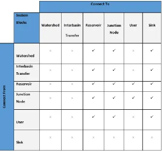
Table 1. Connectivity diagram ... 22

Table 2. Reservoir information. ... 32

Table 3 Wet year TVA reservoir optimization results (Oct. – Dec. 2009) ... 79

(11)

LIST OF FIGURES

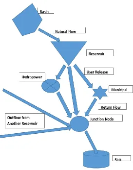
Figure 1. Conceptualization of a reservoir system in GRAPS with major modeling

components ... 9

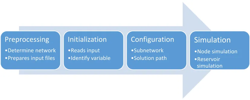
Figure 2. Modules and preparation tasks for setting up the simulation model ... 19

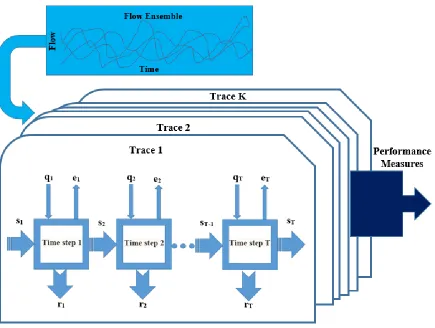
Figure 3. Model execution diagram. ... 20

Figure 4. Inflow and outflow variables allocated with reservoir water balance. ... 23

Figure 5. Jaguaribe valley river and irrigation system. (Not drawn to scale. Adapted from Broad et al., 2007) ... 33

Figure 6. Network diagram of the modeled reservoirs. ... 35

Figure 7. Flow diagrams of inflow and outflow for Node 1, Pacajus and Pacoti for flow routing verification... 38

Figure 8. Simulated storage of each reservoir for the period of July 1993 to March 1994. ... 40

Figure 9. Orós reservoir simulation with zero inflow policy for the water year of 1996. ... 41

Figure 10. Storage reliability curves for Orós reservoir with ensemble streamflow forecast. 43 Figure 11. Map of drought conditions in the U.S. as measured by Palmer Z-Index (“Historical Palmer Drought Indices | Temperature, Precipitation, and Drought | National Centers for Environmental Information (NCEI),” n.d.). ... 57

Figure 12. The GRAPS Framework... 62

Figure 13 Rivers and reservoirs in the Tennessee Valley ... 70

Figure 14. Tennessee Valley watershed. (Hutson et al., 2004)... 71

Figure 15. Tennessee River watershed cascade diagram with modeled reservoir circled in red (Figure not drawn to scale. Modified from Hutson et al., 2004) ... 73

Figure 16 TVA operating guide for Kentucky reservoir (“TVA - Kentucky Operating Guide,” n.d.). ... 75

Figure 17 Elevation storage relationship and storage area relationship curves (Fort Loudoun reservoir) ... 76

Figure 18. PSO convergence plot. (Single runs. Max iteration = 800, Population size = 500) ... 83

(12)

1

MULTIRESERVOIR SIMULATION MODEL

1.1 INTRODUCTION

1.1.1 Challenges and Motivation

Water allocations among municipal, industrial and agricultural sectors require comprehensive integration of supply, demand, climate change and ecological considerations. Many major river systems are extremely regulated with various ecosystem and environmental constraints. Multi-reservoir operations involve allocating supplies of two or more reservoirs to numerous downstream users. Moreover, multi-purpose reservoir operations comprise numerous

interactions and trade-offs among conflicting purposes. For instance, too little release will affect water quality and recreation, too much release will cause flooding. On the other hand, abrupt change in release rate will cause channel erosion and danger for navigation. The conflicting nature of benefits associated with storing the water and benefits associated with releasing the water contributes to the complexity of multi-reservoir system operations.

The goal of the management of a multi-reservoir system is to meet environmental disputes and regulatory (e.g. regulations from Environmental Protection Agency) and physical

constraints and at the same time satisfy water demands by various users. During the course of a reservoir system, the system will likely be subjected to many changes and variations, from external changes such as shifting in climate and deforestation, to internal developments such as adjustment of reservoir rule curve. Reservoir modeling software and programs are

(13)

reservoir modeling tools reservoir managers and operators can simulate different

environments, test out adaptive strategies and inform long-term management policies such as drought contingency plans, and withdraw rates.

Climate change could have a huge impact on watersheds and river basins. For example, higher temperature is found to have lower runoff ratios (Lehner et al., 2017).

Hydroclimatology is a rapidly developing field with exciting result and profound applications to water resources management. Climate phenomena such as El Nino Southern Oscillation (ENSO) have been shown to impact streamflow in many parts of the world (Dettinger and Diaz, 2000). Moreover, streamflow forecasts developed from combining multiple GCMs has been demonstrated to be valuable in reservoir operations (Golembesky et al., 2009). These climate forecasts are represented as ensembles. However, a review of existing literature indicates a paucity in reservoir modeling tools developed with ensemble input in mind. In these contexts, the Civil, Construction, & Environmental Engineering Department at North Carolina State University has developed a reservoir modeling software to address the aforementioned challenges and needs.

1.1.2 Review of Existing Models

(14)

(15)

river basin or multiple-basin region under priority-based water allocation systems. Not only can simulate reservoir system operations for flood control, WRAP can also facilitate

assessments of hydrologic and institutional water availability/reliability in satisfying requirements for instream flows, water supply diversions, hydroelectric energy generation, and reservoir storage. Developed by European research institutes and companies,

(16)

1.1.3 GRAPS

GRAPS stands for Generalized Reservoir Analyses using Probabilistic Streamflow forecasts. It is a newly developed multi-reservoir simulation model by North Carolina State University in Raleigh, NC. The model is based on and extended from a water allocation framework, as described by Arumugam et al. (2003), that utilizes the benefits of ensemble forecasts of reservoir inflows to issue annual water contracts. Applying the water allocation framework on Falls Lake Reservoir, N.C., Golembesky et al. (2009) has demonstrated the usefulness of the framework and multimodel streamflow forecasts in water management. Unlike many mainstream reservoir modeling tool, GRAPS is well suited to handle massive ensemble, which conveys forecast information and related uncertainty, in a speedy fashion. An easy-to-use, generalized, multi-reservoir simulation program, GRAPS can be applied to a myriad of reservoir systems under diverse conditions.

(17)

GRAPS is its capability to take full advantage of advanced forecasts in the form of unwieldly massive ensemble. This new integrated modeling software is developed to alleviate the 21st century challenges faced by water resources professionals and to support complex reservoir decision making.

1.1.4 Outline of the Chapter

This chapter provides detailed descriptions on the simulation program. First, capabilities of the simulation model are introduced. The program is developed by using both node-link formulation approach and object-oriented approach. Reservoirs and users are represented as nodes and are connected by links, which represent channels and rivers. Capable in modeling complex hydrological processes in a real-world reservoir system, GRAPS can represent all major surface water processes and components under a variety of spatial and temporal scales. Features of the program is then presented, which include its ability to handle inflows in the forms of massive ensembles.

Second, methodology in constructing the program is described. How the model is organized and executed are illustrated and explained. The model is executed by stepping sequentially through time and in an upstream to downstream fashion. In addition, mathematical

(18)

formulations are described in detail to elucidate how the model is able to capture the complex behavior of a reservoir system.

Lastly, a case study on reservoirs in Ceará, Brazil to demonstrate GRAPS’ capabilities in reservoir modeling and abilities to accurately reproduce historical storage and flows. Results of the simulation are assessed and validated with historical observations.

1.2 CAPABILITIES

GRAPS is written in Fortran, an established general-purpose, high-level programming language that is well suited for mathematical modeling and scientific computing. Most of the water resources program developed before 1990 and many of the recent ones are written in Fortran (Wurbs, 2005).

(19)

1.2.1 Node-link Formulation Approach

Similar to many other existing water resources systems modeling programs, GRAPS adapted a node-link schematic representation to describe physical river basin networks (not to be confused with network flow programing, a special form of linear programming). Even though shapes of river and reservoir are arbitrary and erratic, the underlying spatial configuration can be simplified and represented in the program by a two-dimensional interconnected directed network of nodes and links.

(20)

Figure 1. Conceptualization of a reservoir system in GRAPS with major modeling

components

1.2.2 Object-oriented Approach

(21)

step t to another state at time step t+1. Such state transition begins when an object such as a reservoir receives information like inflow from upstream. When all the simulations in a network is completed and new state data are recorded, the simulation model can proceed to the next time step. Following the trend and advancement, GRAPS has adapted an object-oriented approach for the modeling of complex multi-reservoir systems.

1.2.3 Modeling Capabilities

Unlike a site-specific reservoir model, GRAPS is designed to be applied to any reservoir systems. Innumerable site-specific reservoir models have been developed during the past several decades; however, these models are not intended for other reservoirs. Because writing testing and debugging code are extremely time consuming and expensive, recently people have been shifting away from customized site-specific models to generalized models (Wurbs, 2005). As a generalized modeling software, GRAPS is designed to model and simulate any reservoir systems under various conditions. Moreover, the modeling of natural systems like watersheds and river systems is complex and requires many assumptions and simplifications to be made. Despite such complexity, GRAPS is able to model all major surface water processes and components of a typical reservoir system.

1.2.3.1 Spatial scale

(22)

system configuration in the nation. From a single reservoir to numerous reservoirs in several basins and based on user defined system, the program is capable of simulating reservoir operations and river flows in arbitrary extents and ranges. Although there have been many studies about climate change impacts on hydrology, many of them are either too broad or two limited. GRAPS can help to bridge this gap by simulating reservoir systems with arbitrary complexities.

1.2.3.2 Time stepping

While many types of reservoir software come with fixed time steps, GRAPS’s overall period and time step of simulation can vary vastly, from monthly to submonthly time step.

Depending on the scope of the study, for example, the time step could be a period of ten years, or a period of three months. Because of this variable time step advantage, GRAPS can be used for daily operation to allow users to replicate short-term system behavior, and can be used for seasonal and yearly operation to simulate system reactions to various management strategies or global warming scenarios. Although GRAPS supports a wide spectrum of time steps, some functionalities may only be useful in a limited range of time steps. In the case of storage routing, daily time step is more appropriate to have over monthly time step.

1.2.3.3 Water supply source

(23)

the main water supply site. In addition, interbasin transfers from other watersheds may also be modeled in the program. As a generic reservoir systems model, GRAPS is well suited for modeling both single reservoir and multi-reservoir systems.

1.2.3.4 Withdrawal and demand

Various withdrawal and demand sites can be modeled via the program. The five main classes of users (stakeholders) in the program are: Municipal, Industrial, Agricultural, Hydropower, and Environmental. After water is allocated to different users, the program is also taking into account return-flows from municipalities and reuse of water downstream.

1.2.3.5 Nodes

There are two major kinds of nodes in GRAPS: reservoir node and junction node. Reservoir node is the place for reservoir simulation. Junction node is more rudimentary and it’s also a place for flow mass balance. Moreover, despite involving no mass balance calculations, basins, users and sinks are also represented as nodes.

1.2.3.6 Links

(24)

While there are innumerable benefits of reservoirs, reservoirs can be harmful to the environment. For instance, thermal stratification (Chapra, c1997.) and eutrophication can happen to reservoirs and impacts water quality. Reservoir releases also impact downstream river and people who value the outdoor environment and use the river for recreational activities. Consequently, GRAPS allows users to specify minimum flow required along a river to meet regulations such as water quality, fish and wildlife, recreation, and navigation.

1.2.3.7 Losses

In the real world, there are numerous kinds of water losses in the natural and manmade environment. Major water losses are represented in the simulation model. Conveyance losses in streams and diversions, as well as consumption losses from users in return flows are both accounted for in the program. Channel losses, such as loss of stream water through

evaporation and infiltration, are represented as fractional coefficients and be specified as inputs. Losses from channels may also be considered in interbasin transfer. Another major form of loss, evaporation from reservoir, is also calculated by using the nonlinear storage-elevation relationship.

1.2.3.8 Junction Node

(25)

multiple reservoirs situate on upstream tributaries. Flexible in modeling, junction nodes can be employed to represent one or multiple physical locations such as gauges or points of river confluences. Junction node can also be used to represent points of withdrawals and points of returns where demand nodes draw water from a river and later return the water back

somewhere downstream.

1.2.3.9 Hydropower

Many major rivers in the United States and around the world are regulated to generate

(26)

1.3 FEATURES

As a generalized model, GRAPS is designed for simulation and subsequent analysis of any basin/river system. The model can be used to represent a reservoir system and simulates its performance under various management and flow forecast conditions. Simulation can be carried out not only on stationary (e.g. historical) scenarios, but also on non-stationary (e.g. climate change) scenarios. Moreover, it can simulate and capture the complexities of operating multiple reservoirs and their intricate interactions due to change in climate or demands. Simulation results encompass major variables such as storage, reservoir releases, releases to users, and hydropower production.

Practical and straightforward to use, the program is designed to engage reservoir managers and watershed stakeholders. Without being concerned with underlying data structure and solvers, users simply need to provide text or data (DAT) file inputs, and inflow time series (historical or forecast) to run the program. Major features of the program are described in the following sections.

1.3.1 Ensemble Input Framework

(27)

benefit reservoir performance. For additional information and methodology about developing streamflow forecasts by using multimodel combination technique, see the forecasting paper by Devineni et al., 2008. As a result of these recent findings and advancements, GRAPS is designed to efficiently handle streamflow input in the form of massive ensemble. By using probabilistic streamflow forecast in the form of ensemble, GRAPS can be used to explored climate change effects on basin management and reservoir systems.

1.3.2 User Interface

1.3.2.1 Input

Like many other advanced water allocation models, GRAPS requires detailed information on basin hydrology, reservoir, and users. For a generalized reservoir model like GRAPS, input files are prepared and tailored to each particular reservoir system. These input files describe the connectivity, reservoir characteristics, reservoir management and user demands of the modeled system. Of these files, the most crucial and fundamental input to the program is appropriately formatted naturalized flow, stream flow that represents natural hydrology, into each reservoir. If there is a lack of inflow data but storage level and release data are

available, inflows into a multi-reservoir system can be estimated based on mass balances (Peng and Buras, 2000).

(28)

water demands for disparate water uses. The user is also expected to provide reservoir system-specific information regarding system and diversion blocks. Specific details about users, such as information about demands and water contracts, are also provided as input.

1.3.2.2 Output

Simulation results encompass major variables such as storage elevation, reservoir releases, releases to users, and hydropower production. The output is typically voluminous (e.g., storage elevation, releases, and diversion flow) and in the form of time series. At the end of each simulation, users can utilize the text output and display results in charts or diagram through a program of their choice. The main result of the program is the reliability of meeting end-of-period target storage for each reservoir.

1.3.3 Scenario

Easy to customize, GRAPS supports scenario analysis to address a wide range of operations and management situations. It also enables the user to quantify the impact of changes in streamflow and management policies. By providing input data that represent different

(29)

1.3.4 Performance Measure

Using a set of scenarios, which can represent a wide range of different operation actions and climate conditions, a measure of performance is needed to easily make comparisons among the scenarios. GRAPS offers the user a variety of ways to measure the performance of the reservoir systems. These performance measures include but are not limited to reliability of water supply to users and reliability of meeting target storage constraints. Express as

percentages, these reliabilities are based on counting the number of times in which a certain criterion (e.g., reservoir storage and volume of water supply) is fulfilled at the end of the simulation.

Reliabilities are formulated as:R n (100%) N

 , where N is the total number of simulation and

n is the number of times a certain criterion is met. Based on the above equation, similar definitions of reliability can be formulated and constructed.

1.3.5 System Requirement

(30)

1.4 METHODOLOGY

1.4.1 Model Composition

The model is comprised of three main parts: initialization, configuration and simulation (Figure 2). The initialization subdivision is for reading input and initializing variables. The configuration subdivision is for automatic constructing of a solution path and translating input into an internal network representation. The most important part is the simulation subdivision, which is for reservoir and flow calculations.

Figure 2. Modules and preparation tasks for setting up the simulation model

1.4.2 Model Execution

The program is executed based on temporal and spatial orders of the calculations. In a node-link representation, all the nodes in a reservoir network are connected by links. For each time step, model simulation starts at the furthest upstream reservoir node and advances according to the constructed solution path. Given a solution path, the simulation progresses

Preprocessing

•Determine network

•Prepares input files

Initialization

•Reads input

•Identify variable

Configuration

•Subnetwork

•Solution path

Simulation

•Node simulation

(31)

in an upstream-to-downstream fashion. During simulation, node simulation module accounts and combines flows from upstream reservoirs and return flows. The reservoir simulation module determines total inflows, evaporation, storage, and releases to downstream reservoirs and users. In these ways, GRAPS is able to track the movement of water from its source watershed to the sink.

Figure 3. Model execution diagram.

(32)

time step 1 to a total of T time steps. Reservoir mass balance calculations (storage, flow and evaporation) occur during each time step. For example, during the time step 1, s1 is the initial storage, q1 is the total inflow, e1 the evaporation, and r1 is the total release to downstream. Thus, the reservoir’s behaviors comprise of transitions from the current state at time t to a

new state at time t+1. Model formulation and mass balance equations are described in detail in later sections.

1.4.3 Connectivity

(33)

Table 1. Connectivity diagram

1.4.4 Model Formulation

GRAPS is a full implementation of a water allocation model as specified by Arumugam et al., 2003. Written in Fortran, GRAPS is hinged on the following mass balance equations and using double-precision floating-point format.

(34)

US including reservoirs that contribute flows indirectly into reservoir-‘s’. Then given this scenario, the flow into any reservoir could be grouped into two categories: (a) Uncontrolled Inflows (b) Controlled flows. Uncontrolled flows are represented in the form of conditional distribution. Two types of uncontrolled flows are considered in the model for the reservoir-‘s’:

(a) Natural Inflowsinto the reservoir (q_{t k}s_, ) (b) Spillagefrom the upstream reservoirs (Ex_ts_,k

).

Controlled flows are of three types: (a) Releases Direct Inflows from upstream reservoirs (b) Return Flows from command areas and wastewater from municipal and industrial use (c) Diversions and water from Inter-basin transfers or from other sources. Controlled flows are expressed as functions of the decision variables of the multi-reservoir water allocation model.

Figure 4. Inflow and outflow variables allocated with reservoir water balance.

Uncontrolled Inflows Controlled Inflows Direct Releases from

Upstream Reservoirs

Return Flows from water uses

Diversions and other transfers

Natural Inflows

Spills from upstream reservoirs

Evaporation

Spill

Releases for uses

Diversions

Direct Release to downstream reservoir

(35)

1.4.4.1 Flow

1.4.4.1.1 Direct Inflow from Upstream Reservoirs:

Direct Inflow results as part of instream requirement as well as excess water being released for hydropower generation and for downstream requirement. This can be expressed as





 US

s s ss t ss s

t a RE

DI 1 ' ' ' ' (1)

Where ss′ is the fraction quantifying the losses on the upstream direct release, REs' , from

reservoir-s′ and

a

_tss' is the within year distribution factor for the direct inflow release.

1.4.4.1.2 Return Flows from Uses:

Assuming there are ‘ns’ uses in each reservoir, releases for each use, Ris, return flows from the

uses released from the upstream reservoirs, US, could be calculated. Let NL be the number of lags (in months) taken for the return flow to reach the reservoir. Then, return flow in month-‘t’ into reservoir-‘s’, RFts can be estimated as,

'

1 ' 1 '

' , ' ' , ' s i U s n i NL t t t s i t ss i t s

t f R

RF s s

 

   

  (2)

where ' '

,

ss i t

f is the fraction of monthly releases from reservoir s′ that contribute into the current

reservoir ‘s’ with the contribution effective from previous releases (NL months) and ' '

,

s i t

 is the

(36)

1.4.4.1.3 Diversions and Other Transfers:

Diversions for wildlife protection and other environmental/inter-basin transfers could contribute to additional inflows.





NDs

d td sd s t D D 1  (3)

sd is the fraction representing the losses in the diverted quantity Dtd. Note Dtd has to be

specified as part of input to the model.

1.4.4.2 Uncontrolled Inflows:

1.4.4.2.1 Natural Inflows:

Natural Inflows, qts,k t = 1, …T is the ensemble probabilistic streamflow forecasts with index

‘k’ representing a particular ensemble.

Spillage:

Spillage is a result of uncontrolled spillway discharge. Net spillage from upstream reservoirs, Ext,k, is the sum of spill from all the upstream reservoirs after accounting conveyance losses.

Spill, ,'

s k t

SP , from reservoir ‘s’ is a derived conditional distribution after accounting releases,

diversions and evaporation.





  Us

(37)

1.4.4.2.2 Net Inflows:

Net inflows, Q_ts_,_k, is the sum of uncontrolled and controlled inflows. Note that RFsandDIs_t

t are

functions of decision variables of the allocation model, whereas Dts has to be specified as an input to the model.

s k t s s t s t s s k

t RF DI D Ex q

Q

k t

t ,

,     ,  (5)

1.4.4.3 Outflows and Releases:

Given the inflow Q_ts_,_kand the reservoir characteristics, we can use the continuity equation to

calculate the controlled releases, diversions, spills and evaporation from the reservoir. Release for Each Use:

Releases for each use is specified as

R

iswhere i=1, .., Ns with a corresponding reliability

(1-pfis) with pf representing the failure probability. Direct Release to Downstream Reservoir

Direct release to downstream reservoir, DIt,s will be obtained as a decision variable in the model.

Diversion and other transfers: Dts

This has to be specified as an input to the model.

1.4.4.4 Reservoir

(38)

Reservoir Information

min

,

max

,

0

s s s

S

are minimum (dead), maximum, initial storages of the reservoir.

H

s

and

SP

maxs

are the elevation of spillway crest level and maximum spillway discharge respectively.

1

and

2

s s



are the storage-elevation curve coefficients of the reservoir.

In line with the water contract specification, different restriction levels, prls, that has to be imposed if the actual inflows are drier than the actual inflows where l = 1,...,nrs denoting the

number of restriction level in a particular reservoir ‘s’.



tsrepresents the monthly evaporation rates in each reservoir ‘s’.

The model attempts to solve the following system of equations. Reservoir Simulation

For each ensemble ‘k’



    

 nr

i ti s t s t s t s

t S Q E R

S

1

1 (6)

which is the main mass balance equation in the program that determines the changes of storage over time in each reservoir. Essentially, the mass balance equation expresses that the change in storage is inflow minus releases and evaporation.

| 0

s s s t t t

SD  S S  (7)

max

min( , ), max( , 0)

s s s s s

t t t t

(39)

Equation (7) calculated shortfall. Equation (8) means the reservoir storage should between its minimum and maximum storages.

ti ti i

R  R (9)

Releases are calculated with demand fractions.

s s t s t s t s t s

t S S

E ₍₍ ₎_/₂₎ 2

1



  _

 (10)

Evaporation at each month,

E

_ts, is calculated as a function of average storage during current

and previous months and by using the storage-elevation relationship. Instead of the more complicated Penman method, which calculates evaporation more accurately but with more parameters (e.g., solar radiation, air temperature and humidity), the above method offers an

acceptable and efficient way for evaporation calculation. Because both s t

S and s t E are

unknown, implicit calculation of evaporation occurs for each member of the ensemble.

1.4.4.5 Hydropower

Hydroelectricity is generated by converting the potential energy of water in reservoirs. Hydropower P is calculated as a function of generator efficiency, K, density of water,,

gravity, g, and height difference between headwater and tailwater elevations, h.

P



K gh



(11)

(40)

hydropower generation for conventional hydropower plants and pumped storage hydropower plants, that obtain energy from potential energy of water stored in reservoirs. Because they have little to no storage, run-of-river hydropower plants’ hydropower generated can’t be determined with the above equation.

Various physical constraints are prescribed in the model. Demand Constraint

,min ,max 1, ...,

s s s

i i i s

R R R s N (12)

Inflow Requirement

' '

,min ,max 1, ...,

s ss ss s

t t t s

DI a RE DI s N (13)

Diversion Demands

,min ,max 1,..., 1, ...,

s s s

t t t s

D D D t T s N (14)

Spillway Constraints

max

(41)

1.5 MODEL APPLICATION

1.5.1 Study Area

1.5.1.1 Jaguaribe Valley, Ceará, Brazil

The purpose of this case study is to demonstrate GRAPS’ modeling capability and ability to accurately simulate historical operations. The case is based on the Jaguaribe River Basin, a river basin situated in the semiarid state of Ceará, in northeast and one of the poorest part of Brazil. With a drainage basin covers an area of 75,961.07 km2, the Jaguaribe River extends for about 610 km and its discharge can range from 7.000 m3_{/s up to zero in a time interval of} few months (Campos et al., 2000). The major water management challenge in the region is to capture the water in reservoirs in rainy years and to manage it such that it will last for several years, in case the following years are drought years (Johnsson and Kemper, 2005). The other important challenge is the increasing dependence of the state capital Fortaleza, one of the largest and fastest growing cities in Brazil (Johnsson and Kemper, 2005).

(42)

1.5.1.2 Modeled Reservoirs

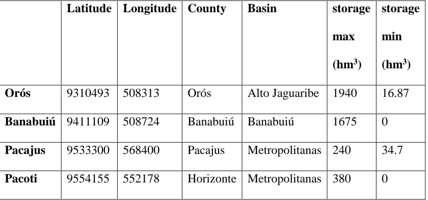
The generalized model is applied to four reservoirs in the Jaguaribe River Basin. The modeled reservoirs in this case study are Orós, Banabuiú, Pacajus and Pacoti. Water is diverted from the Jaguaribe River Basin to the Pacajus reservoir via Canal do Trabalhador (Worker’s Canal). The Canal do Trabalhador is a diversion medium that does supply water to

(43)

Table 2. Reservoir information.

Latitude Longitude County Basin storage max (hm3)

storage min (hm3₎

Orós 9310493 508313 Orós Alto Jaguaribe 1940 16.87 Banabuiú 9411109 508724 Banabuiú Banabuiú 1675 0 Pacajus 9533300 568400 Pacajus Metropolitanas 240 34.7 Pacoti 9554155 552178 Horizonte Metropolitanas 380 0

(44)

Figure 5. Jaguaribe valley river and irrigation system. (Not drawn to scale. Adapted from

(45)

1.5.2 Input

Historical streamflow and reservoir data were provided by Dr. Filho at the Federal University of Ceará, Fortaleza, Brazil. Because the data were provided many years ago, historical inflow and reservoir levels were dated before 2000. Castanhao reservoir, a major reservoir at the region was constructed after 2000. Consequently, Castanhao reservoir was not included in the model.

1.5.2.1 Ensemble input

Because lag-one correlation between the annual flows is close to zero, an ensemble of climatological streamflow forecasts was developed from the historical inflows for the corresponding month from 1913-1995 to populate 1000 ensemble forecasts (Arumugam et al., 2003). This ensemble of forecasts was generated by bootstrapping, a simplistic

resampling technique that draws randomly from a set of data points and allows replacement.

1.5.2.2 Zero inflow policy

(46)

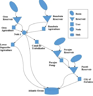
1.5.3 Schematic Representation of the Modeled System

Figure 6. Network diagram of the modeled reservoirs.

Figure 6 illustrates how the multi-reservoir system is represented schematically in the program. The model reservoir network contains reservoirs in both series and parallel

(47)

sector dominates the state and most of the users are agriculture users (as shown in fig. 5.), we simplify the modeling by assigning Orós and Banabuiú to have only one aggregated

agriculture user each. Node 1 (a junction node) is used to represent a point of river confluence and to gather upstream reservoir and user releases from Orós and Banabuiú. Canal do Trabalhador is presented in the network and is modeled as a pump that delivers water from node 1 to the Pacajus reservoir. Due to its function as a small relay reservoir, Pacajus reservoir only has one user, a pump that delivers water from the reservoir to Pacoti reservoir. Finally, Pacoti reservoir supplies all the drinking water to the city of Fortaleza, which is represented as a municipality user node. Although there are two major watersheds, interbasin transfer is not needed as the two watersheds are represented within one system model. Represented as a sink, the Atlantic Ocean receives return flows from Lower Jaguaribe agriculture, node 1, Pacoti reservoir and the city of Fortaleza.

1.5.4 Assumptions

(48)

simplicity, Lower Jaguaribe Agriculture is the only user in the lower Jaguaribe river and represent all the water demands in that area.

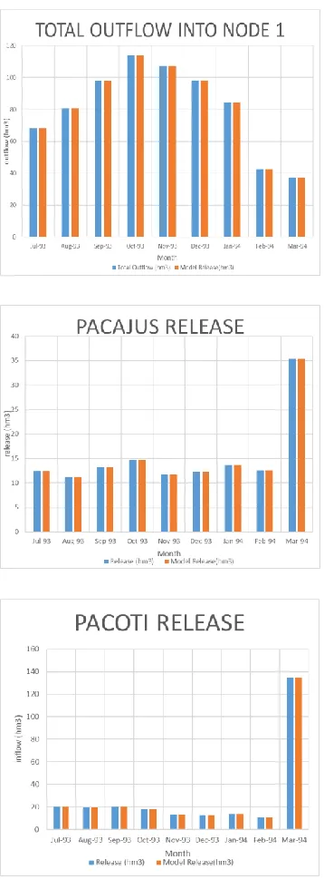
1.5.5 Case Study Simulation Result

(49)

Figure 7. Flow diagrams of inflow and outflow for Node 1, Pacajus and Pacoti for flow

(50)

(51)

Figure 8. Simulated storage of each reservoir for the period of July 1993 to March 1994.

(52)

levels match the historical storage levels and demonstrates the program’s ability to simulate

and reproduce reservoir storage given historical information.

Figure 9. Orós reservoir simulation with zero inflow policy for the water year of 1996.

(53)

reservoir spillages. As a result of Orós in a semi-arid region, Orós reservoir is seldom received enough inflow and is rarely spilled. Hence, zero inflow policy was applied as a conservative measure by the local government and in this case to facilitate and investigate reservoir spillage. Note that in the above historical and zero inflow policy simulations,

(54)

Figure 10. Storage reliability curves for Orós reservoir with ensemble streamflow forecast.

Fig. 10 shows how storage reliability varies as a result of different initial storages for Orós

reservoir (with bootstrapped ensemble forecast input). The storage reliability is calculated by 84 86 88 90 92 94 96 98 100

370 380 390 400 410 420 430 440 450 460 470

R eli abil it y (n/N ) %

Initial Storage (hm3)

Reliability Curve (n/N) % (Orós, 50 hm

3

Target Storage,

440 hm

3

Total Demand)

50 55 60 65 70 75 80 85 90 95 100

0 200 400 600 800 1000 1200

R eli abil it y (n/N ) %

Initial Storage (hm3)

Reliability Curve (n/N) % (Orós, 300 hm

3

Target Storage,

(55)

counting the number of times end-of-period storage equal or above the target storage over the entire traces. Fig. 10 shows two scenarios for Orós reservoir, one with 50 hm3 target storage and another with 300 hm3 target storage. The total demands for both cases are 400 hm3. In both cases, the reliability increases as the initial storage increases. Both figures show the reliabilities increase in steps, instead of gradual increase. This phenomenon is a result of bootstrapped ensemble input. Intuitively, higher target storage will require higher initial storage to achieve the same reliability. This is indeed the case, the model shows that case 1 (Orós with 50 hm3 target storage) only needs 460 hm3 initial storage to attain 100%

reliability, while case 2 (Orós with 300 hm3 target storage) needs about 1100 hm3 to attain 100% reliability.

1.6 SUMMARY AND CONCLUSIONS

(56)

(57)

1.7 REFERENCES

Arumugam, S., Sharma, A., Lall, U., 2003. Water allocation for multiple uses based on probabilistic reservoir inflow forecasts, in: Proceedings of Symposium HS02b Held during IUGG2003. Presented at the Water Resources Systems—Hydrological Risk, Management and Development, IAHS Publ, Sapporo.

Broad, K., Pfaff, A., Taddei, R., Sankarasubramanian, A., Lall, U., de Assis de Souza Filho, F., 2007. Climate, stream flow prediction and water management in northeast Brazil: societal trends and forecast value. Climatic Change 84, 217–239. doi:10.1007/s10584-007-9257-0

Campos et al., 2000 J. N. B. Campos, T. M. C. Studart, R. Luna, S. Franco Hydrological Transformations in Jaguaribe River Basin during the 20th Century In: 20th Hydrology Days, Fort Collins, CO. Proceed-ings of the 20th Annual American Geophysical Union. Fort Collins, Co: Hydrology Days Publications, 2000. v.1. p.221 – 227

Chapra, S.C., c1997. Surface water-quality modeling, McGraw-Hill series in water resources and environmental engineering. McGraw-Hill, New York.

(58)

Dettinger, M.D., Diaz, H.F., 2000. Global Characteristics of Stream Flow Seasonality and Variability. J. Hydrometeor. 1, 289–310.

doi:10.1175/1525-7541(2000)001<0289:GCOSFS>2.0.CO;2

Draper, A.J., Munévar, A., Arora, S.K., Reyes, E., Parker, N.L., Chung, F.I., Peterson, L.E., 2004. CalSim: Generalized Model for Reservoir System Analysis. doi:10.1061/(ASCE)0733-9496(2004)130:6(480)

Golembesky, K., Sankarasubramanian, A., Devineni, N., 2009. Improved Drought

Management of Falls Lake Reservoir: Role of Multimodel Streamflow Forecasts in Setting up Restrictions. doi:10.1061/(ASCE)0733-9496(2009)135:3(188)

Jamieson, D.G., Fedra, K., 1996. The “WaterWare” decision-support system for river-basin planning. 1. Conceptual design. Journal of Hydrology 177, 163–175. doi:10.1016/0022-1694(95)02957-5

Johnsson, R.M.F., Kemper, K., 2005. Institutional and policy analysis of river basin

management : the Jaguaribe river basin, Ceará, Brazil, Policy Research Working Papers. The

(59)

Klipsch, J.D., Hurst, M.B., 2013. HEC-ResSim Reservoir System Simulation User’s Manual.

Labadie, J.W., 2010. MODSIM 8.1: River Basin Management Decision Support System User Manual and Documentation.

Lehner, F., Wahl, E.R., Wood, A.W., Blatchford, D.B., Llewellyn, D., 2017. Assessing recent declines in Upper Rio Grande runoff efficiency from a paleoclimate perspective. Geophys. Res. Lett. 44, 4124–4133. doi:10.1002/2017GL073253

Peng, C., Buras, N., 2000. Practical Estimation of Inflows into Multireservoir System. Journal of Water Resources Planning and Management 126, 331–334.

doi:10.1061/(ASCE)0733-9496(2000)126:5(331)

Sieber, J., Purkey, D., 2015. Water Evaluation And Planning System USER GUIDE.

Singh, V.P. (Vijay P.), Frevert, D.K., 2006. Watershed models. CRC/Taylor & Francis, Boca Raton, FL.

(60)

Wurbs, R.A., 2005. Comparative Evaluation of Generalized River/Reservoir System Models.

Wurbs, R.A., 2015. Water Rights Analysis Package (WRAP) Modeling System Reference Manual.

Yao, H., Georgakakos, A., 2001. Assessment of Folsom Lake response to historical and potential future climate scenarios: 2. Reservoir management. Journal of Hydrology 249, 176– 196. doi:10.1016/S0022-1694(01)00418-8

Zagona, E.A., Fulp, T.J., Shane, R., Magee, T., Goranflo, H.M., 2001. RIVERWARE: A GENERALIZED TOOL FOR COMPLEX RESERVOIR SYSTEM MODELING1. JAWRA Journal of the American Water Resources Association 37, 913–929. doi:10.1111/j.1752-1688.2001.tb05522.x

Stroustrup, B., 1988. What is object-oriented programming? IEEE Software 5, 10–20. doi:10.1109/52.2020

Sulis, A., Sechi, G.M., 2013. Comparison of generic simulation models for water resource systems. Environmental Modelling & Software 40, 214–225.

(61)

2

MULTIRESERVOIR OPTIMIZATION MODEL

2.1 INTRODUCTION

2.1.1 Challenges and Motivation

As global population is expected to keep growing exponentially and countries are expected to keep advancing and developing, the demand of energy is escalating. Under this context, clean energy plays a considerable role in not only meeting energy demands, but also combating global warming and climate change. A major renewable energy, hydropower is an

inexpensive way of generating energy to meet various demands (e.g. peak load and base load). The leading renewable source for generating electricity, hydropower supplies about 70% of all renewable electricity and generates about 16% of total energy (Radu and Ibeanu, 2017). Although reservoirs also emit a significant volume of greenhouse gases (Deemer et al., 2016), hydropower plants are still less harmful than fossil fuel plants in polluting the air. Besides hydroelectricity generation, multi-purpose reservoirs are also used for drinking water supply, irrigation, and flood control. Given the complexity and assortment of challenges faced by water and energy professionals, optimization model can be used to solve today and tomorrow’s pressing water and energy management problems.

The utility of water resources optimization models has been displayed in numerous studies. For instance, by using an economic-engineering optimization, Jenkins et al. (2004) were able to make significant improvements for California’s water supply system through water

(62)

enormous success of applying optimization models to solve reservoir management problems in theories, actual real-world implementations remain limited or have not been sustained (Labadie, 2004).

Moreover, given the challenges of urbanization, technology uncertainty, resource constraints, and the threat of climate change, a better cyberinfrastructure is needed for the better

management of nation’s reservoir systems. Under these challenges, GRAPS (Generalized

Reservoir Analyses using Probabilistic Streamflow forecasts) has been further refined and developed to include the ability to optimize reservoir systems.

2.1.2 Review of Optimization Techniques for Reservoir Operations

“… [O]ne of the most important advances made in the field of water resources engineering is

the development and adoption of optimization techniques for planning, design, and

(63)

engineering. Typically, DP models are developed for specific reservoir system instead of being generalized for any systems (Wurbs, 2005). Recently, numerous heuristic

programming methods have been developed and applied extensively in the field of water resources engineering. For example, Cai et al. (2001) applied genetic algorithms (GA) for solving large nonlinear water management problems. More recently, multi-objective

optimization techniques have been subjected to intense study and applied extensively to the field of water resources management. Interested readers can read about the rich literature of reservoir optimization from the classic reservoir management and model review by Yeh, 1985, and a state-of-the-art multi-reservoir system optimization summary review by Labadie, 2004.

Even though most of the mathematical programming techniques mentioned in the review section can be applied to solving nonlinear problems, many of them have major flaws. For dynamic programming, the main problem (computational) is the notorious curse of

dimensionality. Many methods were developed to alleviate the dimensionality problem, such as incremental dynamic programming (IDP) and dynamic programming successive

approximation (DPSA), but they fail to eliminate the problem completely (Labadie, 2004). Equivalent reservoir is another method of tackling the dimensionality problem of DP by aggregating all reservoirs into one. However, the problem with such state

(64)

together (Labadie, 2004). For chance constrained programming, researchers had doubted the practical usefulness of the technique in modeling (Hogan et al., 1981).

2.1.3 Review of Existing Optimization Models

Numerous sectors, from government agencies and universities, to engineering companies and consulting firms, contributed to the development of diverse reservoir optimization models. Many of the models mentioned in the model review section in Chapter 1 are capable of optimization. For instance, Riverware has been used by TVA and USBR (United States Bureau of Reclamation) for short-term scheduling and long-term planning (Zagona et al., 2001). Similar to WRAP, most models for water allocation systems are based on network flow programming (Wurbs, 2005). In addition, many detailed site-specific models have been developed. For example, an economic-engineering optimization model for California’s water resources, CALVIN was showed to improve California’s water supply system operation and

water allocations with an expected value as large as $1.3 billion per year (Jenkins et al., 2004). For more information about various established reservoir optimization software, see model comparison and review by Wurbs, 2005.

2.1.4 GRAPS

(65)

real-world applications of reservoir optimization models, Labadie (2004) suggests one of the keys to success in implementing reservoir optimization model is to improve linkage with

simulation models. GRAPS offers ways to not only simulate varying changes but also optimize in a timely fashion.

Modeling approaches that include human actions have been widely recognized by the water resources scientific community to be beneficial in understanding the movement of water (Brown et al., 2015). GRAPS implemented water contract as described in Arumugam et al., 2003, which includes management elements like reliability of meeting target storages and penalty for not meeting water user demands. As a result, reservoir operations involve competing goals like maximizing revenue from multiple users and minimizing penalty for not meeting minimum storage and instream flow constraint.

GRAPS is implemented by using the simulation and optimization approach. Under such an approach, an optimization model is coupled with a simulation model. Two methods are available to solve nonlinear reservoir operation problems. The first method is particle swarm optimization (PSO), a global population-based optimization method inspired by the

(66)

2.1.5 Outline of the Chapter

This chapter introduces the optimization component of GRAPS. First, capabilities of the newly developed multi-reservoir optimization model are presented. The optimization model is based on the previously developed simulation model with the same name, which can accurately reproduce reservoir storage variation and correctly route inflow and outflow from upstream to downstream. Despite the immense and numerous reservoir and multi-reservoir modeling programs in the academia and industry today, programs that can effectively take advantage of ensemble input are few and far between. One of the advantages of GRAPS is that the program is being developed with ensemble flow input in mind and the program can capitalize the massive ensemble that can be easily generated nowadays.

Second, the simulation and optimization model is formalized and described in detail. During this section, various performance measures are described, water contract is introduced, as well as formulation of the objective function is presented. Nonlinear functions are

(67)

Last but not least, the capabilities of the model are demonstrated by applying the program to the TVA (Tennessee Valley Authority) reservoir system. A federally owned corporation, TVA owns and operates hydropower plants in the Tennessee Valley. Tennessee is a southeastern state with large hydropower production and a state plagued by hydrologic disasters such as droughts. The valley of Tennessee, where most of the reservoirs are located, experienced severe drought in 2016 (Figure 11) with some part of the region declared a rare Exceptional Drought (D4) by the National Oceanic and Atmospheric Administration (“TN Valley Drought in 2016,” 2017). In monthly time step, 28 reservoirs in the Tennessee Valley

is modeled and represented in the program. The system-wide model is optimized in both dry and wet year cases. At the end of the case study, optimum water allocation from each

(68)

Figure 11. Map of drought conditions in the U.S. as measured by Palmer Z-Index

(“Historical Palmer Drought Indices | Temperature, Precipitation, and Drought | National

(69)

2.2 CAPABILITIES

2.2.1 Climate Information Based Streamflow Forecasts

Streamflow forecasts based on climate information provides a considerable amount of opportunity in the development of short-term water management strategies and in setting up contingency measures for the threats of extreme climate events such as drought and floods. GRAPS is aimed at combining improved hydroclimatic information obtained from

hydrologic forecasting models to aid in improving water-related management decisions.

(70)

2.2.2 Simulation and Optimization

Simulation and optimization modeling approach is used to solve thorny water resources problems. Under this approach, an optimization model uses a simulation model to predict a modeled system’s responses under a specified set of states. Repeat runs of a simulation

model can be used to iteratively search for maximum objective and assess the performance of a system under varying inputs and assorted conditions. Under such approach, the simulation model can be used to answer “what if” questions and the optimization model can be used to answer “what is the best” questions under a specific set of situations (Singh, 2014).

Simulation and optimization modeling approach has a long history of applications in the field of civil and environmental engineering. Search methods are used to iteratively finding better values as determined by an objective function. A review of simulation and optimization modeling for sustainable irrigation uses of surface and groundwater resources is examined by Singh, 2014. Based upon the recently developed simulation model as detailed in Chapter 1, GRAPS effectively combines both simulation and optimization models under a unified framework.

2.3 FEATURES

2.3.1 Input

(71)

are read in from a file. The inflows are represented in an n-column matrix, in which n is the number of time steps. It is recommended to use monthly time step and to use monthly averages. In addition, each row represents an “ensemble” list of forecast inflows, and each entry corresponding to the inflow of a particular time step. Similar to the simulation model, additional detailed information about the watershed, reservoir, and demand are also required to be prepared and used as input into the program.

2.3.2 Analysis

GRAPS provides two methods of analysis: one is retrospective analysis and another is real-time operation analysis. Retrospective analysis allows the user to analyze the potential benefits of using climate information-based streamflow forecasts in relation to the

climatological information/currently followed practice. Real-time Operation allows the water manager to obtain monthly/seasonal decisions with regard to water allocation and reservoir operation by updating the reservoir system information to current conditions and utilizing the recently updated streamflow forecasts

2.3.3 Water Contract

(72)

(73)

2.4 METHODOLOGY

Figure 12. The GRAPS Framework.

2.4.1 Software Architecture

(74)

optimization, the framework drives the multi-reservoir simulation model under different decision variables.

2.4.2 Water Contract Formulation

A water supply contract for use ‘i’ is described by: (a) Duration, T

(b) Total volume of water, Ri, to be delivered over the contract period (c) Within period demand fraction, βti

(d) Amount, fi, to be paid for the water if all contract terms are met (e) Target reliability, (1-pfi)

(f) Restrictions, wi*, that the supplier can impose as part of the contract if the inflows are lesser than forecast

(g) Restriction fraction, αij, signifying the reduced supply under restriction level ‘j’ (where j = 1, …, nr with nr is the total number of restriction levels agreed by the

water committee)

(h) Compensation amount, γij, for the contract holder if restriction level ‘j’ is imposed (i) Compensation schedule, vi, for the contract holder in the event of contract failure

(i.e., if the total possible restriction is inadequate to meet the shortfall in the forecasted streamflow).

(75)

Total deficit,D, is computed by: 1 T s s t t D SD 





(16)

i

w for user “i” is calculated from CDil, restriction for user “i” in restriction level “l”.





 nr

l s il s i CD w 1 (17)

For a more detailed description of the water contract, please see Arumugam et al., 2003. Meanwhile, the probabilities are computed by looking at all the traces in the ensemble:

1. P(wis wi,maxs ) as the number of traces in which wis wi,maxs / total number of traces N

2. P(STsSTrs) as the number of traces in which STsSTrs / total number of traces, N

3. P(RLls) as the # of traces in which restriction level ‘l’ is enforced / total number of traces, N.

On top of the physical based constraints described in Chapter 1, there are additional management constraints.

Reliability Constraints:

,max

(ws_i ws_i ) ps_fi 1,..., N_s 1,..., N_s

P   i s (18)

(76)

Restriction Level Enforcement:

(RL )s_l pr_ls 1,..., _rs 1,..., _s

P  l n s N (19)

End of the Time Period Storage Constraint:

(STs S )Trs ss 1,..., s

P  p s N (20)

STrs is the target end of the time period storage and pss is the associated failure probability.

2.4.3 Objective Formulation

The objective of the program is to maximize the net utility from multiple uses.

O = ,max

1 1 1 1 1 1

(

)

(S

S )

s s l

N n N n n n

s s s s s s s s s

i i il il i i i Tr T

s i s i j i

R

W









     















 











 



In which i denotes the value of each use and

      Otherwise x if x 0 0 1 ) ( .

Consequently, the multi-objective problem of maximizing benefits and minimizing penalties is in the form of a single objective function. For a minimization solver like the one in Optimus, signs in the above equation are flipped to suit the solver.

2.4.4 Solvers

(77)

storage relationship. Instead of linearizing these functions and using piece-wise linear approximation, nonlinear programming techniques and algorithms are employed in the program. Furthermore, owing to the deficiencies in aforementioned mathematical

programming procedures, heuristic programming techniques such as PSO are better suited for a simulation-optimization program. Like other genetic algorithms, a major advantage of PSO is that it can be linked directly with trusted simulation model (Labadie, 2004). The two methods employed by GRAPS, PSO and FSQP are described in the following sections.

2.4.4.1 Particle Swarm Optimization (PSO)

2.4.4.1.1 Standard PSO

(78)

value and the optimum value (if known) is less than the maximum tolerance or the maximum number of evaluations is reached (Clerc, 2012).

2.4.4.1.2 PSO with Penalty Method

Application of PSO to constrained problems requires penalty method to transform the problems into an unconstrained one. As a result, constraints are embedded into the objective function with varying penalties that penalize constraint violations. One drawback of the penalty method is the introduction of free variables into the problem. In the objective function, a penalty coefficient is attached to each kind of constraint. These penalty coefficients are arbitrary and chose relatively to the objective by trial and error. Thus, the larger the constraint violation the higher the penalty for that violation.

2.4.4.2 Feasible Sequential Quadratic Programming (FSQP)

FSQP is a set of FORTRAN subroutines for the minimization of the maximum of a set of smooth objective functions subject to general smooth constraints (Zhou and Tits, 1992).

(79)

There are several limitations of FSQP. Because the algorithm is mainly for smooth problems, it will likely to have difficulty in solving non-smooth functions (Zhou and Tits, 1992).

Additionally, FSQP might be slow for problems with “thin” or unusually shaped feasible sets (Zhou and Tits, 1992). Moreover, SQP has the problems of having indefinite quadratic programming subproblems and being effective in solving only certain classes of large-scale nonlinear problems (Morales et al., 2012). Because the above limitations, FSQP is intended to function as an auxiliary method to the main PSO solver.

2.5 MODEL APPLICATION

2.5.1 Study Area

In this case study, the study area is the Tennessee Valley Authority watershed. Established by the Tennessee Valley Authority Act during the Great Depression, TVA owns and manages reservoirs and hydropower plants in the Tennessee Valley. In addition to hydropower generation, TVA also manages power productions from its many nuclear and fossil fuel power plants and operates them to serve a large electricity grid. Covering seven states, the Tennessee Valley watershed is about 40000 mi2 in size.

2.5.1.1 Hydrologic Setting of the Tennessee Valley Watershed

(80)

Carolina, Tennessee, and Virginia (Hutson et al., 2004). From east to west, the Tennessee River originated from Appalachian Mountains of Virginia and North Carolina. The Tennessee River flows westward passing through major cities such as Knoxville,

(81)

Figure 13 Rivers and reservoirs in the Tennessee Valley

2.5.1.2 Water Uses of the Tennessee Valley Watershed

(82)

for modeling watersheds like the TVA watershed with roughly 98% surface water withdrawals (Bohac and Bowen, 2012).

2.5.1.3 Modeled TVA Reservoirs

There are 28 reservoirs in the model with a wide range of characteristics. The smallest reservoir in terms of storage is Wilbur, with a maximum storage of only 0.715 TAF. On the other hand, the largest reservoir is Kentucky, with a maximum storage of a whopping 6129

(83)

(84)

Figure 15. Tennessee River watershed cascade diagram with modeled reservoir circled in

(85)

2.5.2 Input

2.5.2.1 Dry and Wet Years

Two hydrologic cases, dry and wet years, are included in this demonstration. 2007 and 2009 are the two years determined by calculating the average monthly precipitation anomalies from the norm.

2.5.2.2 Data Source

(86)

Figure 16 TVA operating guide for Kentucky reservoir (“TVA - Kentucky Operating Guide,”

(87)

Figure 17 Elevation storage relationship and storage area relationship curves (Fort

Loudoun reservoir)

Above figures show the elevation storage relationship and storage area relationship curves for Fort Loudoun reservoir as an example. Coefficients for elevation storage relationship and storage area relationships were determined from such Excel trendline equations for all reservoirs.

y = -0.0004x2_{+ 0.3276x + 750.63} R² = 0.9608

730 740 750 760 770 780 790 800 810 820 830

0 100 200 300 400 500 600