www.ijiset.com
Kernel Based Extreme Learning Machine in Identifying
Dermatological Disorders
Krupal ParikhP 1
P
, Trupti ShahP 2
P
1
P
Department of Applied Science & Humanities, G. H. Patel College of Engineering & Technology, Gujarat Technological University Vallabh Vidyanagar, Gujarat-388120, India
P
2
P
Department of Applied Mathematics, Faculty of Technology & Engineering, M.S. University of Baroda, Vadodara, Gujarat-390001, India
Abstract
Extreme Learning Machine (ELM)has gained importance among various learning algorithms particularly related to multi classification problems. In this paper, kernel-based ELM is used to identify common skin disorders such as Bacterial Infection, Fungal Infection, Eczema and Scabies. A proper diagnosis of these diseases at primary stage is very essential to prevent future complications. The various kernel functions like Radial Basis Function, Polynomial kernel, Exponential Chi-Square kernel with ELM are applied on the skin dataset. In our study we measure accuracy and leaning time obtained using these kernels with ELM and Support Vector Machine (SVM). We also analyze our dataset on Conventional Single Layer feed Forward Network (SLFN). A comparative study of accuracy and learning time of all these learning algorithms is made and it is observed that ELM gives optimum learning time with good classification accuracy using exponential chi-square kernel.
Keywords: 27TExtreme Learning Machine, Single Layer Feed Forward Network, Support Vector Machine, Skin Diseases, Exponential chi-square kernel, Classification.
1.
Introduction
Extreme Learning Machine (ELM) was originally developed for single hidden layer feed forward neural network-SLFN[1].Artificial Neural Network (ANN) based classifiers can integrate both structural and statistical information and achieve better performance than that of minimum distance classifiers[2].However, conventional feed forward neural network use gradient descent method to train network, which might get the algorithm stuck at local optimum. Also, all parameters of the network need to be tuned iteratively, so learning speed is very slow [1]. ELM is a single layer feed forward neural network (SLFN), which randomly chooses input weights and analytically determines the output weights. When input weights are taken arbitrary and hidden neurons are specified, SLFN is considered as linear system and output weights are calculated analytically. This makes learning speed of the network extremely fast. According to Bartlett SLFNs tend to have good generalisation performance if it not only minimizing training error but also having smaller norms of weights [3]. The learning algorithm of ELM not only
www.ijiset.com much time in adjusting parameters during training. So, in
DL training speed is very slow. In [13] convolutional extreme learning machine with kernels (CKELM) was proposed. The hidden layer of CKELM is not single layer but adds convolution layers and subsampling layers. It is based on DL but do not use gradient descent algorithm to adjust parameters. It uses random weights during training. Thus, CKELM uses features of convolution neural network (CNN) with ELM. So, in CKELM features are extracted with less training time.
Skin diseases such as Bacterial Infections, Fungal Infections, Scabies and Eczema are very common in developing countries. In [14] Parikh & Shah discussed the importance of proper diagnosis of these diseases at primary stage. In [14], authors used ANN with single as well as with two hidden layers and SVM with RBF and Polynomial kernels to diagnose these diseases. In [15] authors used the same data set and obtained classification accuracy with various kernels using SVM. In this paper we use ELM with Polynomial kernel functions, Radial Basis Function and Exponential chi-square kernel function to diagnose these diseases and obtain good classification accuracy with less learning time compare to SVM.
The rest of the paper is organized as follows. We review Machine learning techniques namely Conventional single hidden layer feed forward neural network (SLFN), Extreme learning machine (ELM) and Support vector machine (SVM) in section 2. We also present a comparative study of various features of SLFN, ELM and SVM in this section. Data description, Experiments and result analysis are discussed in section 3. Conclusion is given in section 4.
2.
Machine Learning Techniques
2.1
Conventional Single Hidden Layer Feed
Forward Neural Network(SLFN)
Feed forward neural networks were very popular learning algorithm in 90’s because of their ability to approximate complex nonlinear functions and provide model for many natural and artificial phenomena.
It consists of one layer of input nodes, one layer of hidden nodes and one layer of output units. In conventional feed forward networks input weights and hidden layer biases need to be adjusted. More over the learning algorithm use gradient descent method, which is generally slow and an improper learning step may lead to local minimum. SLFNs for N arbitrary distinct samples
(
xi,Ti)
where[
]
T nin i i
i x x x R
x = 1, 2,... ∈ and Ti =
[
ti1,ti2,...tim]
T∈Rmwith hn hidden units and activation functiong
( )
x , the output is mathematically calculated as(
i j i)
j ni i
o b x w g h
= + ∑
=1 .
β , j=1, 2,...,N
where wi =
[
wi1,wi2,...win]
T is the weight vector connecting the ith hidden node and the input nodes,[
]
Tim i
i
β
β
β
β
= 1, 2,... is the weight vector connecting theth
i hidden node and the output nodes, bi is the
threshold for the ith hidden node. To train an SLFN, values ofwi ,bi,βi
(
i=1,2,...,nh)
are to be train insuch a way that the cost function
(
)
∑
∑ + −
=
= =
N
j n
i i i j i j
h
t b x w g E
1
2
1
.
β is minimum.
Here g
( )
x is an activation function such as sigmoid function, radial basis function, sine, cosine, exponential function and many other nonregular functions [16]. In order to minimize cost function, conventional SLFN use gradient based algorithms and weights are iterativelyadjusted as
( )
w w E w
wk k
∂ ∂ −
= −1
η
where η is thelearning rate. If η is very small then learning time is
very large and if η is very large then algorithm is unstable and there may be a risk of divergence. Another drawback of the learning algorithm is that it may stop in local optimum. But, these draw back can be overcome using ELM.
2.2
Extreme Learning Machine (ELM)
ELM is also single hidden layer feed forward network, where hidden layer need not be neuron alike. In ELM input weights wi and biasesbi
(
i=1,2,...,nh , whereh
n be the number of hidden nodes) are assigned randomly.
Hidden nodes are crucial but need not be tuned in ELM. They are randomly initiated and remains unchanged ([1],[7]). Also, ELM maintains universal approximation capability even though hidden nodes are provided arbitrarily.
For N arbitrary distinct samples
(
xi,Ti)
where[
]
T nin i i
i x x x R
x = 1, 2,... ∈ andTi =
[
ti1,ti2,...tim]
T∈Rm , n is number of features and m is number of classes, the objective is to find the weight vector[
]
T n mnh ∈R h×
= β β β
β 1, 2,... which minimize
0
2=
−T
H
β
with minimum norm of output weightβ
. There are two stages for ELM training.www.ijiset.com continuous activation function g
( )
x such as sigmoidfunction, Gaussian function and many more. For ELM hard limit and multiquadratic also give good generalization performance [19]. For activation function one may use kernel functions such as Radial Basis Function, Polynomial kernel, Exponential chi-square kernel etc. The hidden nodes map input nodes to feature map. The hidden node weights are randomly generated. They are independent of training instances.
The hidden layer output matrix
( )
(
)
(
)
(
)
(
)
+ + + + = h h h h n N T n N T n T n T b x w g b x w g b x w g b x w g x h 1 1 1 1 1 1In the second stage, weights
[
1, 2,..., n]
Th β β β =
β , which
connects hidden layers with nodes nRhR to output nodes
(m≥1) are obtained by
Minimizing H
β
−T 2 = ∑(
)
∑ + − = = N j n
i i i j i j
h t b x w g 1 2 1 . β
The objective function of ELM is given by,
∑ − + = N i T H C 1 2 2 2 2 1
min β β
β ,
where C is a regularization parameter which is the trade off between norm of output weights and the training error
T H
β
− .The objective of the ELM is not only to minimize training error but also find optimum solution with minimum norm. Thus, it tends to have good generalization performance.[3] . If the number of training samples N and the number of hidden nodes nh are equal, then the hidden matrix H is
square and invertible. But, in most cases nh << N. In this case H is not a square matrix and the linear system
0 = −T
H
β
can be solved using Moore-Penrose inverse. The output layer weight βare estimated by the following equation: T H C I H H TH T T
1 * + − + = = β ,
where I is h×h identity matrix,T=
[
t1,t2,...,tm]
T∈RN×mis the target vector. H+is the Moore-Penrose generalized
inverse of the matrix H. H+T can be solved using Gaussian elimination method, orthogonal projection method, iterative method etc.
.
2.3
Support Vector Machine(SVM)
SVM was originally developed by Vapnik in 1995[18]. It is based on statistical learning theory. It is also called large margin classifier. It was originally developed for binary classification, but, it can be use for multi classification using one to one or one to all techniques. It can classify nonlinear function using kernel function. It uses kernel trick in which, in the feature space no need to calculate highly non linear kernel functions. Instead due to kernel trick only scalar product is required in feature space. In feature space it finds optimal separating hyper plane by solving quadratic programming optimization problem. For N training samples
(
)
{ }
{
xi,yi ,xi∈Rn,yi∈ −1,1i=1,2,...,N}
, the objective function is to minimize∑ ξ + = N 1 i 2 i 2 C w 2 1 , with
(
w.x b)
1 , 0 i 1,2,3,...N.yi i+ ≥ −ξi ξi≥ ∀ =
where Cis a positive constant, which is the trade off between marginal error and testing error .
Solving dual problem of this quadratic problem, optimum value of w can be obtained, which maximize the margin by the separating hyper plane
w
⋅
x
+
b
=
0
and the decision function is given by( )
(
)
+ ∑ α =∈ ykx ,x b
sign x
f i i
SV
i i
,
where training sample xiwith corresponding non zero αi
is called support vector( )SV . k
( ) () ( )
.,x =φ..φ x is called kernel function. Kernel plays a very important role in performance of SVM [19]. Most popular kernel functions are Radial Basis Function, Polynomial kernel, Sigmoid kernel etc.Differences and Relationship of various Features of Traditional SLFN, ELM and SVM are summarized in Table 1.
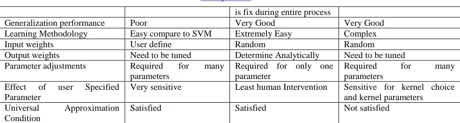
Table: 1 Comparison Study of features of Conventional SLFN, ELM and SVM
SLFN ELM SVM
Optimum value Local Optimum Global Optimum Global Optimum
Computing Time High Very Low High
Multi classes Single ANN for m classes Single ELM for m classes m or m(m-1)/2 for m classes Affected by Sample
Complexity
No No Yes
www.ijiset.com
is fix during entire process
Generalization performance Poor Very Good Very Good
Learning Methodology Easy compare to SVM Extremely Easy Complex
Input weights User define Random Random
Output weights Need to be tuned Determine Analytically Need to be tuned
Parameter adjustments Required for many
parameters
Required for only one parameter
Required for many
parameters Effect of user Specified
Parameter
Very sensitive Least human Intervention Sensitive for kernel choice and kernel parameters
Universal Approximation Condition
Satisfied Satisfied Not satisfied
3.
Data Description, Experiments and Result
Analysis
In our study we apply learning algorithm to diagnose common skin diseases such as Bacterial Infection, Fungal Infection, Scabies and Eczema. The data was collected from Department of Skin & V.D., Shrikrishna Hospital, Karamsad, Gujarat, India. Our dataset contains 470
patients’ information. Each patient is investigated using 47 features. Out of 470 samples, 139 samples are of Bacterial infection, 146 are of Fungal Infection, 98 are of Eczema and 87 are of Scabies. The attributes information use in analysis is given in Table 2.
Table 2: Input Attributes used for Analysis
Chief Complaints & OPD
1. Pain 2 Fever 3. Itching
Seasonal relation
4. Summ 5 Winter 6. Monsoon
Past History
7. Diabetes 8 Family History Occupational History
9. Hot and humid environment 11 Excessive sun exposure 10.. Exposure to irritants
Type of Lesion
12. Macules 16 Nodule
13. Patches 17 Plaques
14. Papules 18 Vesicles
15. Pustule 19 Bullae
Colour
20. Erythematous 22 Hypopigmented 21. Hyperpigmented
Associated With
23. Lichenification 26 Scaling
24. Oozing 27 Excoriation
25. Crusting 28 Discharge
Shape
29. Linear 30 Annular 31 Grouped
Sites
32. Webspaces 37 Abdomen 42 Back
33. Wrist 38 Genitals 43 Buttocks
34. Forearm 39 Thigh 44 Palms & Soles
35. Arm 40 Legs
36.. Chest 41 Dorsa of feet
www.ijiset.com
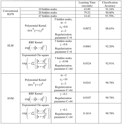
For comparative study, we use conventional SLFN and SVM along with ELM. Table 3 summarizes learning time and accuracy, when above three learning algorithms are applied on the data set.
In each case, we use 70% data for training and 30% data for testing purpose. Partitions are done by random process. All simulations for SLFN, ELM and SVM are carried out in MATLAB R2015b running in i5-44605 CPU @ 2.90GHz. Results are finalized taking averages of 100 trials. For SLFN, we use Neural Network toolbox of MATLAB. The network is created using
newff() matlab inbuilt function. We use ‘logsig’ as activation function. Training is done using Levenberg-Marquardt algorithm. Results are taken for 10, 20 and 47 hidden nodes in hidden layer. In ELM, classification accuracy is obtained using Polynomial kernel, RBF kernel and Exponential chi-square kernel. Parameters are set using grid search algorithm. For SVM also we use same kernels as in ELM. In SVM classification was done using LIBSVM 3.20 with MATLAB interface [20]. To decide parameters, we use 10 fold cross validation.
Table 3: Performance result of Conventional SLFN, SVM and ELM for 70-30% data partition
Learning Time (seconds)
Classification Accuracy Conventional
SLFN
10 hidden nodes 43.89 91.24%
20 hidden nodes 79.52 90.60%
47 hidden nodes 14.42 93.70%.
ELM
Polynomial Kernel
d 1 T
) c y x (α +
5 hidden nodes, α=1
1
c =0.8
d=3 Regularization parameter C=8
0.0072 88.65%
RBF Kernel
−γ − 2
y x exp
5 hidden nodes γ=0.8 Regularization parameter C=8
0.0061 92.20%
Exponential Chi-square
∑
+ − γ −
2 2
y x
y x exp
5 hidden nodes γ=0.98 Regularization parameter C=64
0.0324 92.91%
SVM
Polynomial Kernel
d Ty c)
x (α +
α=2
1
c =10
d=3 Regularization parameter C=64
0.0241 90.78%
RBF Kernel
−γ − 2
y x exp
γ=0.1 Regularization parameter C=64
0.0187 90.78%
Exponential Chi-square
∑
+ − γ −
2 2
y x
y x exp
γ=0.1 Regularization parameter C=64
0.1614 90.78%
4.
Conclusions
The simulation results show that the accuracy obtained using Conventional SLFN is highest among the three learning algorithms under study. But it may be due to local optimum. We also find that using SLFN, learning
www.ijiset.com accuracy, ELM is taking about 398% less learning time
than that of SVM for the data set under study. So, we observe that ELM has better scalability compared to SLFN and SVM.
Acknowledgments
Authors are thankful to Shrikrishna Hospital to give permission for data collection. Authors are also thankful to the department of Skin & VD for their help to collect data.
References
[1] G. B. Huang, Q.Y. Zhu , and C.K. Siew, “Extreme learning machine: theory and applications”, Neurocomputing, Vol.70, no. 1, pp. 489-501, Dec. 2006.
[2] W. Zhao, R. Chellappa, P.J. Phillips, and A. Rosenfeld, “Face recognition: A literature survey”,ACM computing surveys (CSUR), Vol. 35,no.4, pp. 399-458, Dec.1, 2003 [3] P. L. Bartlett, “ The sample complexity of pattern
classification with neural networks: the size of the weights is more important than the size of the network”, IEEE transactions on Information Theory, Vol. 44,no. 2,pp. 525-536, Mar. 1998.
[4] G. -B. Huang, X. Ding, and H. Zhou, “Optimization method based extreme learning machine for classification,” Neurocomputing, vol. 74, no. 1–3,pp. 155–163, Dec. 2010. [5] G. -B. Huang, and L. Chen, “ Convex incremental extreme
learning machine”, Neurocomputing , Vol. 70, no.16, pp.3056–3062, Oct. 31, 2007.
[6] G. -B. Huang, L. Chen, “ Enhanced random search based incremental extreme learning machine” , Neurocomputing, Vol. 71, no. 16, pp. 3460-3468, Oct., 31, 2008.
[7] G. Huang, G. -B. Huang, S. Song, and K. You, “Trends in Extreme Learning Machine: A Review”, Neural Network, Vol. 61, pp. 32-48, Jan. 2015.
[8] G. -B. Huang, H. Zhou, X. Ding, and R. Zhang, “Extreme learning machine for regression and multiclass classification”, IEEE Transactions on Systems, Man, and Cybernetics, Part B (Cybernetics), Vol. 42, no. 2, pp. 513-529, Apr. 2012
[9] X. Liu, L. Wang, G.B. Huang, J. Zhang, and J. Yin, “Multiple kernel extreme learning machine”, Neurocomputing, Vol.149, pp.253-264, Feb. 3, 2015.
[10]Y. Wang, F. Cao, and Y. Yuan, “A study on effectiveness of extreme learning machine”, Neurocomputing, Vol. 74, no. 16, pp. 2483-2490, Sep. 30, 2011.
[11]G. E. Hinton, S. Osindero, and Y. W. Teh, “A fast learning algorithm for deep belief nets”, Neural Computing, Vol. 18, no. 7, pp.1527–1554, Jul. 2006.
[12]G. E. Hinton, and R. R. Salakhutdinov, “Reducing the dimensionality of data with neural networks”, Science, Vol. 313, no. 5786, pp. 504-507, Jul. 28, 2006.
[13]S. Ding, L. Guo, Y. Hou, “Extreme learning machine with kernel model based on deep learning”, Neural Computing and Applications, pp. 1-10, 2016.
[14]K. Parikh, and T. Shah,”Diagnosing Common Skin Diseases using Soft Computing Techniques”, International Journal of Bio-Science and Bio-Technology, Vol. 7, no. 6, pp. 275-286, 2015.
[15]K. Parikh, and T. Shah, “Support Vector Machine - a Large Margin Classifier to Diagnose Skill Illnesses” , Procedia Technology Elsevier Publisher, Vol. 23, pp. 369-375, 2016. [16]G.-B. Huang, and H. A. Babri, “Upper bounds on the
number of hidden neurons in feedforward networks with arbitrary bounded nonlinear activation functions”, IEEE Trans. Neural Networks, Vol. 9, no.1,pp. 224–229, 1998. [17]G.-B. Huang, Q.-Y. Zhu, K. Z. Mao, C.-K. Siew, P.
Saratchandran, and N. Sundararajan, “Can threshold networks be trained directly?” IEEE Trans. Circuits Syst. II, Exp. Briefs, vol. 53, no. 3, pp. 187–191, Mar. 2006.
[18]C. Cortes, and V. Vapnik, “Support-vector networks”, Machine learning, Vol. 20, no. 3, pp. 273-297. Sep. 1,1995. [19]Y. Zhang, P. Fu, W. Liu, and G. Chen, “Imbalanced data
classification based on scaling kernel-based support vector machine”, Neural Computing and Applications, Vol. 25, no. 3-4, pp. 927-935, Sep. 1, 2014.
[20]C. C. Chang, C.J. Lin, “LIBSVM: a library for support vector machines”, ACM Transactions on Intelligent Systems and Technology (TIST), Vol. 2, no. 3, pp.27, Apr. 1,2011.
Krupal Parikh, received Master of Science in Applied Mathematics from M. S. University of Baroda, India. She is working as an Assistant Professor in the department of Applied Science and Humanities, G. H. Patel College of Engineering & Technology, Gujarat, India and also pursuing Ph.D. in Applied Mathematics from M. S. University of Baroda. Her current research of interest includes soft computing techniques and its applications in medical informatics.
Trupti Shah received Ph.D.(Applied Mathematics) from M.S.University of Baroda, Vadodara and P.G. Diploma in Computer Science and Application (P.G.D.C.A.) from the Sardar Patel University, Vallabh Vidyanagar. She is working at Department of Applied Mathematics, M.S. University of Baroda since 1994. Her research work includes controllability and stability problems of discrete dynamical systems using functional analytic techniques. Her interest includes soft