Lists in a Lighthouse

(1)

University of South Carolina

Scholar Commons

Theses and Dissertations

Winter 12-14-2015

nD − PDPA: n Dimensional Probability Density

Profile Analysis

Arjang Fahim

University of South Carolina

Follow this and additional works at:https://scholarcommons.sc.edu/etd

Part of theComputer Engineering Commons, and theComputer Sciences Commons

This Open Access Dissertation is brought to you by Scholar Commons. It has been accepted for inclusion in Theses and Dissertations by an authorized administrator of Scholar Commons. For more information, please [email protected].

Recommended Citation

Fahim, A.(2015).nD − PDPA: n Dimensional Probability Density Profile Analysis.(Doctoral dissertation). Retrieved from

(2)

nD−P DP A_: n _{Dimensional Probability Density Profile Analysis}

by

Arjang Fahim

Bachelor of Science

Azad University of Tehran, 1998 Master of Science

University of South Carolina, 2014

Submitted in Partial Fulfillment of the Requirements

for the Degree of Doctor of Philosophy in

Computer Science

College of Engineering and Computing

University of South Carolina

2015

Accepted by:

Homayoun Valafar, Major Professor

John Rose, Committee Member

Marco Valtorta, Committee Member

Gabriel Terejanu, Committee Member

Mirko Hennig, External Committee Member

(3)

c

(4)

Dedication

This dissertation is dedicated to all the people who have brought so much into

my life.

To my wife, without you this journey might not have been successful. Thanks for

your emotional and intellectual support. With all my love, I dedicate this dissertation

to you.

To my daughter, you have brought more into my life than you can imagine. I

have become a better person, because of the reflection of myself I see in your eyes.

To the day you will be a fabulous woman, I dedicate this dissertation to you.

To my mother, whom I missed her so much. You gave me the love and confidence

to believe I could achieve anything. For always being in my heart, I dedicate this

(5)

Abstract

Proteins are often referred as working molecule of a cell, performing many

structural, functional and regulatory processes. Revealing the function of proteins

still remains a challenging problem. Advancement in genomics sequence projects

produces large protein sequence repository, but due to technical difficulty and cost

related to structure determination, the number of identified protein structure is far

behind. Novel structures identification are particularly important for a number of

reasons: they generate models of similar proteins for comparison; identify

evolution-ary relationships; further contribute to our understanding of protein function and

mechanism; and allow for the fold of other family members to be inferred.

Consider-ing the evolutionary mechanisms responsible for the generation of new structures in

proteins, it has been speculated that there may be a limited number of unique protein

folds as few as ten thousand families. Currently, the Protein Data Bank consists of

nearly 113,000 protein structures, but less than 1,500 families are represented, and

almost no new fold families have been reported since 2008. Ideally, solved protein

structures for new protein families would be used as templates for in silico structure

prediction methods, and the results of both solved and predicted structures would

in turn be used to infer function. However, such an approach requires new, efficient

and cost-effective computational methods for target selection and structure

determi-nation. Traditional characterization of a protein structure by NMR spectroscopy is

expensive and time consuming regardless of the structural novelty of the target

pro-tein. In an effort to expand the applicability of NMR spectroscopy, the community

(6)

enable the study of more challenging, or structurally novel proteins. While many

ad-vances have been made in this regard, very little attention has been made on reducing

the cost of structural characterization of routine proteins.

Probability Density Profile Analysis (PDPA) has been previously introduced to

directly addresses the economies of structure determination of routine proteins and

subsequently, identification of novel structures from minimal sets of NMR data. The

latest version of PDPA (2D-PDPA) has been successful in identifying the structural

homologue of an unknown protein within a library of 1000 decoy structures. In

order to further expand the selectivity and sensitivity of PDPA, incorporation of

additional data is necessary. However, current PDPA approach is limited by its

computational requirements, and its expansion to include additional data will render

it computationally infeasible. Here we propose a new method and developments

that eliminate PDPA’s computational limitations and allow inclusion of Residual

Dipolar Coupling (RDC) data from multiple vector types in multiple alignment media.

Additionally nD-PDPA will be used to refine an unknown protein to obtain closer

(7)

List of Tables

Table 4.1 PDP analysis of the structure 1C99(79) with 20 different

struc-tures representing 9 family folds. . . 39

Table 4.2 Results of PDP analysis to experimental data collected from

Galentic3 (PDBID:1A3K(137)) . . . 41

Table 5.1 List of four proteins that are used in establishing the properties

of 2D-PDPA bb-rmsd interpretation patterns . . . 48

Table 5.2 Results of structure identification using simulated data. . . 50

Table 5.3 Results of structure identification from unassigned experimental

RDC data for the protein PDBID:1P7E. . . 51

Table 5.4 Results of structure identification from unassigned experimental

RDC data for the protein PDBID:1RWD. . . 52

Table 5.5 Pairwise bb-rmsd of the ten structures modeled by ROBETTA

and five structures modeled by I-TASSER. . . 54

Table 5.6 Order tensors of PF2048.1 estimated from 2D-RDC analysis us-ing unassigned RDC data from two alignment media (Phage and

PEG). . . 55

Table 5.7 2D-PDPA scores for the ten ROBETTA structures. . . 56

Table 5.8 2D-PDPA scores for the five I-TASSER structures. . . 56

Table 5.9 Results of 2D-PDPA analysis of modeled structures for PF2048.1 with the estimated range of bb-rmsd to the solution state

struc-ture using 1A1Z(91) as a template for the interpretation pattern. . 58

Table 6.1 List of the protein structures that are used for the experiment.These structures are obtained from Protein Data Bank. . . 65

Table 6.2 List of initial order parameters generated by REDCAT that are

(11)

Table 6.3 Order Tensor parameters estimation using 2D-Approx software for the data listed in Table 6.2. The data is corrupted by±1Hz

of error and 25% of the RDCs are removed from datasets. . . 66

Table 6.4 Summary of the results of 1OUR using RDC sets without any error (second column) and RDC sets with ±1Hz error and 25%

of RDC values randomly removed(third column) . . . 70

Table 6.5 Summary of the results of 1G1B using RDC sets without any error (second column) and RDC sets with ±1Hz error and 25%

of RDC values randomly removed(third column) . . . 70

Table 6.6 Protein structures that are obtained from BMRB database based

on availability of experimental RDC. . . 71

Table 6.7 This table shows the QFactor for 5 N-H RDC sets for protein 1P7E. 71

Table 6.8 List of relative Order Tensor values estimated for M1 and M2 with respect to M1. Also M3 and M4 with respect to M3 for

protein 1P7E. . . 72

Table 6.9 The estimation of the Order Tensor values for three sets of

ex-perimental N-H RDC using 3DApprox software for protein 1P7E. . 72

Table 6.10 The nD-PDPA scores for the first ten structures of Figure 6.11(b). The RDC sets that are used in this experiment are M1 and M2.

Both RDC sets are N-H vectors. . . 75

Table 6.11 The nD-PDPA scores for the first ten structures 6.11(c). The RDC sets are used in this experiment are M1, M2 and M3. All

RDC sets are N-H vectors. . . 75

Table 6.12 List of relative Order Tensor values estimated for M1 and M2 with respect to M1. Also M3 and M4 with respect to M3 for

protein 1P7E. . . 76

Table 7.1 The result of refinement from Figure 7.2 is listed here. The second column shows the iteration (Run) number. 7th column

(12)

Table 7.2 The detail refinement process result from Figure 7.3. Column one denotes the iterations number followed by the best candidate structures name in column two. Columns three to six indicate the orientation of the molecule and the rotation axis in which the best nD-PDPA score produced. Column seven is nD-PDPA score for each iteration and the last column is the bb-rmsd with

respect to 1A1Z protein. . . 82

Table 7.3 The detail refinement process result from Figure 7.4. Column one denotes the iterations number followed by the best candidate structures name in column two. Columns three to six indicate the orientation of the molecule and the rotation axis in which the best nD-PDPA score produced. Column seven is the nD-PDPA score for each iteration and the last column is the bb-rmsd with

respect to 1D3Z protein. . . 85

Table 7.4 The detail refinement process result from Figure 7.5. Column 1 denotes the iterations number followed by the run number in column 2. Columns 3 to 4 indicate the orientation angles of the molecule and the rotation axis in which the best nD-PDPA score produced. Column 5 is the nD-PDPA score for each iteration

and the last column is the bb-rmsd with respect to 1P7E protein. . 86

Table 7.5 The result of ranking of an refinement iterations. Run1 shows 3.051Å while Run2 shows the better bb-rmsd. In this case struc-tures from row2 to row 12 are selected as reference strucstruc-tures for

the next refinement iteration. . . 88

Table 7.6 The result of nD-PDPA refinement using n-Best structures selec-tion method. Each group is separated by a blank line, indicate a refinement iteration. The gray shaded structures indicate the best structure among n best structure in each iteration. The

structure refinement shows improvement of 1.5Å. . . 89

Table 7.7 The result of the comparison of the nD-PDPA with the xPlor-NIH. The Starting Structure column denotes the bb-rmsd of the structure with respect to protein 1A1Z. And Refined Structure column shows the bb-rmsd of the refined structures with respect

to 1A1Z. . . 91

Table 7.8 The result of comparison of nD-PDPA with xPlor-NIH. The Starting Structure column denotes the bb-rmsd of the structure in Å with respect to protein 1D3Z. And Refined Structure col-umn shows the bb-rmsd of the refined structures with respect to

(13)

(14)

List of Figures

Figure 1.1 The Structure of a prototypical amino acid. The chemical groups bound to the centralα−carbon, are highlighted in the background. The R-group represents any of the possible 20

amino acid side chains. . . 2

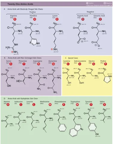
Figure 1.2 The twenty amino acids used in proteins. Each amino acid is labeled by its full name followed by three letters and one letter (in the red circle) abbreviations. Amino acids are grouped into negative or positive charges, hydrophobic or hydrophilic side

chains [71]. . . 3

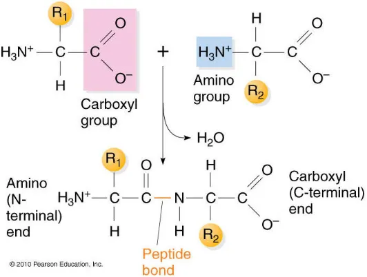
Figure 1.3 Peptide bond formation between successive amino acids. Amine group ends on the second (R2) amino acid is added to the car-boxyl end of the first (R1) amino acids. The amino acid termi-nus of R1 amino acid remains unchanged, end of polypeptide grows in theN toCdirection. The repeatingN−C(R)−C

sub-unit remaining after the dehydration is an amino acid residue [71]. 4

Figure 1.4 The backbone atoms of two joined amino acids.The green spheres

denote the carbon atoms and the blue spheres are nitrogen atoms. 4

Figure 1.5 The planar characteristic of the peptide bond, and the rotation of the peptide backbone about the Cα atom. The two planar

peptide bonds about the central α−carbon, shown here as a ball-and-stick model. Rotation is only possible aroundφ and ψ

angles. . . 5

Figure 1.6 A schematic representation of a ramachandran plot (a plot of

φ andψ angles). The closed regions denotes valid regions forφ

and ψ angles. The red dots are φ and ψ angles extracted from database of 50 structures. Data was taken from Richardson Lab

(http://kinemage.biochem.duke.edu) . . . 6

Figure 1.7 Comparison of Ramachandran plots for Proline and Glycine amino acids. The smaller side-chain of Glycine demonstrates the larger valid region φ and ψ in contrast to Proline and

(15)

Figure 1.8 (a) Atomic formation of an α − helix, the red dashed lines represent the hydrogen bonds that form the helix shape.(b) The

cartoon view of the same helix. . . 8

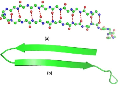
Figure 1.9 (a) Atomic formation of aβ−sheet, red dashed lines represent the hydrogen bonds that form β−sheet.(b) The cartoon view

of the same β−sheet. . . 9

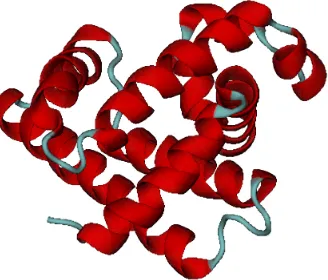
Figure 1.10 Tertiary representation of the protein 1G1B(164). . . 9

Figure 1.11 Homomeric quaternary representation of the protein 1NWW(149). 11

Figure 1.12 Superposition of human and the yeast FK506-binding proteins 2FKE(107)(red) and 1YAT(113)(green) the backbone RMSD score for the backbone atoms after alignment is 0.887 Å. These

proteins have very similar structures. . . 12

Figure 2.1 Myoglobin (PDBID:1MBN(153)). This protein is very common in muscle cells, and its function is to store Oxygen. The reserved Oxygen is used when muscle tissues are hard at work. It is

characterized using X-ray crystallography in 1958. . . 15

Figure 2.2 The illustration of diffraction of incoming beams when colliding

with crystal points.( [93]) . . . 16

Figure 2.3 Protein BUS2(57) is known as the first de-novo protein

charac-terized by NMR spectroscopy . . . 17

Figure 2.4 caption for LOF . . . 18

Figure 2.5 Number of protein structures in PDB (a) unique folds reported

by SCOP and (b) cumulative since 1992 . . . 20

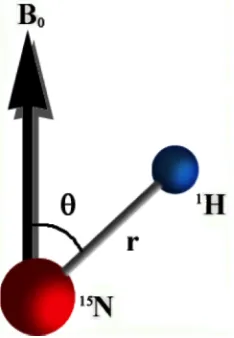
Figure 3.1 The dipolar coupling between two nucleiN andHthat depends

on the distance r and average orientation θ. . . 24

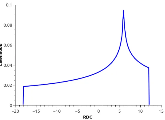
Figure 3.2 Sample powder pattern for the Residual Dipolar Coupling. . . 25

Figure 3.3 Distribution of simulated RDCs for protein 1A1Z(91) (in red-dotted color), with hypothetical order tensors. The horizontal axis represents value of RDC data and the vertical axis

(16)

Figure 4.1 A powder pattern and the PDP for ARF (PDBID: 1HUR(180)) using principal order parameters of -71.1, 47.4 and 23.7 in units

of Hz. . . 33

Figure 4.2 An example of Parzen density estimation using Gaussian kernels

applied to four points. . . 35

Figure 4.3 Distribution of simulated RDCs for protein 1A1Z(91) (in red-dotted color), with hypothetical order tensors. The horizontal axis in this figure represents value of RDC data and the vertical

axis represents the likelihood of observing a given value of RDC. . 36

Figure 4.4 General flowchart of the PDPA algorithm. . . 37

Figure 4.5 Structure of all 12 proteins used in the application of PDP

analysis of Galectin3 (PDBID:1A3K(137)). . . 40

Figure 5.1 An example of a 2D-PDP map generated using kernel density

estimation. This 2D-PDP can serve as a structural fingerprint. . . 44

Figure 5.2 Operational schematic of the 2D-PDPA method illustrated in

three main phases. . . 45

Figure 5.3 Sensitivity of 2D-PDPA analysis as a function of bb-rmsd when applied to (a) two unrelatedα-proteins and (b) two unrelated b-proteins. Simulations included addition of±0.5 Hz of uniformly

distributed noise. . . 48

Figure 5.4 Sensitivity of 2D-PDPA analysis as a function of bb-rmsd on twoα-proteins 1A1Z(91) and 2M67(81) (a) with 25% of the data

randomly removed and (b) with 30% of the data randomly removed. 48

Figure 5.5 Cartoon representation of proteins 1P7E(56) (yellow), 1IGD(61)

(blue) and 1P7F(56) (red). . . 51

Figure 5.6 Cartoon representation of the superimposed structures 1BRF(53)

(yellow) and 1RWD(53) (blue). . . 52

Figure 5.7 Fifteen modeled structures of PF2048.1 by ROBETTA and

(17)

Figure 5.8 Results of 2D-RDC analysis based on unassigned data from PF2048.1 obtained in Phage and PEG alignment media. The blue lines indicate the convex hull of the 2D-RDC dataset de-termined from the experimental data and the red line indicates the convex hull of the distribution of 2D-RDC data points for

the order tensor estimate. . . 55

Figure 5.9 An interpretation patter for the protein PF2048.1, which illus-trates the relationship between 2D-PDPA’s score and structural

quality in bb-rmsd. . . 57

Figure 6.1 An example of a 2D-PDP map, using kernel density estimation. This 2D-PDP can serve as a structural finger print.M1 and M2

denote RDC sets from two alignment media. . . 61

Figure 6.2 2D-PDPA utilizes a 64 by 64 grid for both computational and experimental RDC sets for scoring. The out of boundaries area

are unnecessary for calculation. . . 63

Figure 6.3 cartoon representation of the proteins used in the experiment . . 64

Figure 6.4 (a) Calculated nD-PDPA scores vs. bb-rmsd for protein 1G1B using two N-H RDC sets. (b) Calculated nD-PDPA scores vs.

bb-rmsd for protein 1G1B using two N-H and Cα-Hα RDC sets. . 67

Figure 6.5 The funneling pattern of nD-PDPA score and bb-rmsd of 1000 decoy structures for protein 1A1Z(83). Three N-H RDC sets

were used to conduct this experiment. . . 67

Figure 6.6 250 decoy structures (1A1Z as reference) with (a) two N-H RDC sets (2D-PDPA) (b) three N-H RDC sets (nD-PDPA). 25% of

the data were randomly removed from each set. . . 68

Figure 6.7 (a) Calculated nD-PDPA scores vs. bb-rmsd for protein 1G1B using two N-H RDC sets. (b) Calculated nD-PDPA scores vs.

bb-rmsd for protein 1G1B using two N-H and Cα-Hα RDC sets. . 69

Figure 6.8 Calculated nD-PDPA scores vs. bb-rmsd for protein 1G1B uti-lizing three sets of RDC. Two of which are N-H sets and the third one is Cα-Hα. R2 value is improved in comparison to

utilization of two RDC sets. . . 69

(18)

Figure 6.10 The plots of nD-PDPA and 2D-PDPA analysis using 250 decoy structures for protein 1P7E. All RDC sets are experimental and Order Tensor values are calculated using REDCAT software.(a) 2D-PDPA analysis using { NH, NH } vectors from two align-ment media;(b)nD-PDPA analysis using { NH, NH } vectors from two alignment media;(c)nD-PDPA analysis using { NH,

NH, NH } vectors from three alignment media(M1, M2 and M3) . 73

Figure 6.11 The plots of nD-PDPA analysis utilizing 250 decoy structures for protein 1P7E. All RDC sets are experimental and Order Tensor values are estimated using 2D and 3D approximation software. (a){ NH-NH} RDC vectors from two alignment me-dia (M1 and M2);(b){ NH-NH } RDC vectors from two align-ment media (M2 and M3);(c){ NH-NH } RDC vectors from

three alignment media (M1, M2 and M3); . . . 74

Figure 6.12 The plots of nD-PDPA analysis utilizing 250 decoy structures for protein 1D3Z. All RDC sets are experimental and Order Tensor values are estimated using 2D and 3D approximation software (a){NH-NH}RDC vectors from two alignment media;(b){ NH, CαHα}RDC vectors from two alignment media;(c){NH, CN } RDC vectors from two alignment media;(d){ NH, NH,

CαHα } from two alignment media. . . 77

Figure 7.1 Operation schematic of refinement illustrated in three main stages. 79

Figure 7.2 The refinement process of a modeled structure that is 2.847Å away from 1A1Z. The red dots denotes the structure with the best nD-PDPA score at each round. Totally this refinement ran in six iterations. The final structure is approximately 1.9Å away from 1A1Z. Two N-H RDC sets with no error is used for

this experiment. . . 81

Figure 7.3 The refinement process of a modeled structure that is 2.847Å away from 1A1Z. The red dots denotes the best structure at each iteration. Totally this refinement ran in 6 iterations.Final structure is about 1.7Å away from 1A1Z. Three N-H RDC sets

with no error is used for this experiment. . . 82

Figure 7.4 The refinement process of a structure that is 2.843Å away from protein 1D3Z. The experiment is repeated 22 times using

(19)

Figure 7.5 The refinement plot of a structure that is 2.911Å away from the

protein 1P7E. The experiment is repeated 15 iterations. . . 86

Figure 7.6 The superimpose of four structures from Table7.4.The struc-tures include Run0 in blue, Run6 in red, Run8 in purple and Run10 in green. The reference structure, protein 1P7E also is

added in cyan. . . 87

Figure 7.7 Three out of nine shaded structures from Table 7.6 and 1D3Z are superimposed. 1D3Z is in cyan, the reference (row 1) is in

red, the row 2 is in green and the row 8 is in blue. . . 90

Figure 8.1 A fragment of the configuration file for nD-PDPA. The align-ment media count and the information about the RDC type

and order tensor values are shown. . . 94

Figure 8.2 A fragment of the configuration file for nD-PDPA is demon-strated. Setting information for Kernel calculation such as

sigma and start and end rotational angles are shown. . . 95

Figure A.1 The flowchart of the decoy structures generator program. . . 114

Figure A.2 The distribution of the bb-rmsd for 1000 decoy structures from

protein 1A1Z. . . 115

Figure A.3 The distribution of the bb-rmsd for 5000 decoy structures from

(20)

Chapter 1 Proteins: The building block of life

1.1 Fundamentals of Protein Structures

Almost all biological processes involve the interaction of one or more proteins. These

large molecules exhibit a remarkable versatility that allow them to perform a myriad

of crucial activities and functions. Structure of proteins is not separate from their

functionality. It has been shown that there is a relation between the protein

struc-ture and its functionality. Many reactions in biological systems are conducted by

proteins, producing a sophisticated chemical reaction that an organism needs for its

life. Moreover, proteins have the responsibility of transporting chemicals and

regu-lating functions in organisms. Proteins are polymers constructed from a set of 20

amino acids. Polymers of amino acids are called polypeptide.A protein may consist of one or more polypeptides chain that are folded into a specific three-dimensional

shape [50] [71].

1.1.1 The Primary Structure of Proteins: Sequence

of Amino Acids

A protein is a linear combination of amino acids and this combination ultimately

defines its three-dimensional shape. The sequence of amino acids is often called

(21)

Figure 1.1: The Structure of a prototypical amino acid. The chemical groups bound to the centralα−carbon, are highlighted in the background. The R-group represents any of the possible 20 amino acid side chains.

formula of an amino acid. At the center of an amino acid, there is a carbon atom

called α−carbon. Surrounding the α−carbonare an amine group, carboxyl group,

hydrogen atom and a variable group symbolized by the letter R. The R group is

called the side chain and is different for every amino acid. There are nearly 20 amino

acids that can be incorporated into a protein sequence. The resulting protein can

use any number of 20 amino acids, in any order. Physical and chemical properties of

the side chain determine the characteristic of an amino acid such as hydrophobicity,

hydrophilicity, and polarity (Figure 1.2).

1.1.2 The Peptide Bond

When two amino acids are positioned in such a way that the carboxyl group of the

first amino acid links with the amine group of the other, the result is a dehydration

reaction where a water molecule is formed and removed from the reaction and the

two amino acids come together to form a covalent bond called apeptide bond (Figure 1.3).A polypeptide is synthesized by linear formation of peptide bonds between two

(22)

(23)

Figure 1.3: Peptide bond formation between successive amino acids. Amine group ends on the second (R2) amino acid is added to the carboxyl end of the first (R1) amino acids. The amino acid terminus of R1 amino acid remains unchanged, end of polypeptide grows in the N to C direction. The repeating N −C(R)−C subunit remaining after the dehydration is an amino acid residue [71].

Figure 1.4: The backbone atoms of two joined amino acids.The green spheres denote the carbon atoms and the blue spheres are nitrogen atoms.

(24)

Figure 1.5: The planar characteristic of the peptide bond, and the rotation of the peptide backbone about the Cα atom. The two planar peptide bonds about the

central α−carbon, shown here as a ball-and-stick model. Rotation is only possible aroundφ and ψ angles.

1.1.3 Ramachandran plot

The peptide bonds have important effects on the three-dimensional structure of

a protein. These bonds are labeled as φ (Phi) and ψ (Psi) angles (Figure 1.5). The

peptide bonds give a polypeptide limited freedom to rotate only about theα−carbon

bond. The limitation of the rotation of theφ(N−Cα) andψ (Cα−C) angles are due

to steric hindrance between the side chain of the residue and the peptide backbone. A

Ramachandran Plot (a plot ofφ vs ψ angles) maps the entire allowed and disallowed conformational space of an amino acid. These restrictions were developed by G.N

Ramachandran in the late 1960s based on studies of sterically allowedφandψtorsion

angles (Figure 1.6). An amino acid with the simple structure in the side chain (e.g

Glycine with a single hydrogen(Figure 1.2)) demonstrates less steric hindrance of φ

andψwhich leads to expanding the conformational space. On the other hand, Proline

(with a cyclic R group (Figure 1.2)) demonstrates less freedom of steric hindrance

(25)

Figure 1.6: A schematic representation of a ramachandran plot (a plot of φ and ψ

angles). The closed regions denotes valid regions for φ and ψ angles. The red dots are φ and ψ angles extracted from database of 50 structures. Data was taken from Richardson Lab (http://kinemage.biochem.duke.edu)

1.1.4 The secondary structure of a proteins: Local

Three dimensional structures

The stability that is introduced by hydrogen bonds leads to locally stabilized

con-formations that are known asSecondary Structures. The secondary structure consists of polypeptide chains that repeatedly coils or folds into a pattern that contributes

to a protein’s overall conformation. The two types of secondary structure that are

dominant in protein conformation areα-helix and β-sheets.

1.1.5 α

-Helices

(26)

Figure 1.7: Comparison of Ramachandran plots for Proline and Glycine amino acids. The smaller side-chain of Glycine demonstrates the larger valid region φ and ψ in contrast to Proline and Pre-Proline.Generally the larger side-chain restricts backbone movements.

residues in anα−helixis the geometrical relationship. In an α−helix any residue

i + 1 rotates approximately 100◦ rotation relative to the residue i around the helix axis. α−helicesin protein, almost without exception, are right handed. If the chain

is compressed more tightly than in an α −helix, an alternative hydrogen-bonded

structure can form, called the 310 helix, whereN−H of residuei is hydrogen bonded to the carbonylO of residuei+3. If the chain winds up less tightly than theα−helix, it can form aπ−helices, in which theN−H of residue i is hydrogen bonded to the carbonyl O of residuei+5.

1.1.6 β

-sheets

A β−sheet is formed from two separate strands, which may arise from regions

(27)

Figure 1.8: (a) Atomic formation of an α−helix, the red dashed lines represent the hydrogen bonds that form the helix shape.(b) The cartoon view of the same helix.

residue side chains alternating position on the opposite sides of the sheet (Figure

1.9). The two possible arrangements for β−sheets are parallel and anti-parallel. In

parallel sheets, the strands are arranged in the same direction with respect to the

amine terminal (N) and carboxyl terminal (C) ends. However, in the anti-parallel

arrangement, the strands alternate the amino acid and carboxyl terminal ends in such

a way that a given strand interacts with a strand in the opposite direction.

1.1.7 The tertiary structure of proteins: Global

three-dimensional structure.

Tertiary structure of a protein is defined as the global three-dimensional structure

of its polypeptide chain (Figure 1.10). Tertiary structure of a protein is the result

of interaction between the side chains (R group) of the various amino acids.

Con-sequently, the side chains in the tertiary structures of a protein play an important

(28)

Figure 1.9: (a) Atomic formation of a β −sheet, red dashed lines represent the hydrogen bonds that form β−sheet.(b) The cartoon view of the sameβ−sheet.

Figure 1.10: Tertiary representation of the protein 1G1B(164).

responsible for the generation of the secondary structure (α−helixand β−sheet).

1.1.8 Protein folding

The process of transferring the linear polypeptide chain to a three-dimensional

structure is referred as protein folding. Protein folding is a complex process that is

(29)

properties (such as hydrgenbonds, van der Waals interactions, backbone torsion

an-gles preferences and etc) of linear set of amino acids translate to the three-dimensional

native conformation of a protein and what forces drive amino acids chain into a folded

structure [32]. The physical forces are described byforcefields. The forcefields utilize internal potential energy of proteins for computer simulations. Although computer

aided simulation methods such as MD (Molecular Dynamic) Simulation are successful

to address the folding problem, but so far, such a modeling succeeds on small and

simple protein folds [67]. More complex protein structures require more

computa-tional power and speed, which is still out of reach of our computacomputa-tional capabilities.

Most proteins probably go through many intermediate states to reach to the final

stable folded stage; and looking at the mature conformation does not reveal the stage

of the folding required to achieve the final conformation.

1.1.9 The Quaternary structure of proteins

Quaternary structure of a protein is the aggregation of two or more folded

polypep-tides into its functional macro-molecule. These proteins are also referred as

multi-subunits. The subunits may be identical (homomeric) proteins or they can be

con-stituted of different proteins subunits (hetromeric)(Figure 1.11).

1.2 Classification of Protein Structures

Protein structures can be categorized based on the similarity in sequence, topology

or even in observable structural details. Protein sequence and topology similarity

are two main features that are utilized in protein classification. As the number of

characterized protein structures grew, the classification of these proteins became more

difficult [64] [29] [30]. A protein fold family is a group of proteins that share common

(30)

Figure 1.11: Homomeric quaternary representation of the protein 1NWW(149).

or structure. When a novel protein is identified, its functional properties can be

potentially predicted based on the group to which it belongs. It is worthy to note

that the classification of a novel protein solely based on the sequence may not always

lead to a correct classification if three-dimensional conformation of the structure is

not considered [50]. In the classification of protein, it is also important to study the

biological evolutionary of the structure. The terms super-family (describing a large group of distantly related proteins) andsub-family(describing a small group of closely related proteins) are sometimes used in this context.

1.2.1 Comparison of proteins using sequences and

struc-tures

A common method to identify the similarities of proteins is comparing protein

sequences. If the sequence of amino acids of two proteins aligns, then either the

(31)

Figure 1.12: Superposition of human and the yeast FK506-binding proteins 2FKE(107)(red) and 1YAT(113)(green) the backbone RMSD score for the backbone atoms after alignment is 0.887 Å. These proteins have very similar structures.

similarity between amino acids can be used. The similarity between two sequences is

then the sum of the value of the indices of similarity for each pair of aligned amino

acids plus a correction to address for insertion and deletion of amino acids [51] [33].

Given the structures of two proteins, it is possible to superimpose the

three-dimensional structures using computer tools to observe the similarities and differences

of the structures. A commonly used mathematical measure of the difference between

two structures is rmsd (root-mean-square deviation) in atomic position of the back

bone atoms after optimal super position (Figure 1.12).

1.2.2 Classification of protein topologies

Classification based on the topology was first proposed by M. Levitt and C.

Chothia [63]. This classification is based on the secondary and tertiary structures

(32)

Usu-ally domains are responsible for a particular function or interaction, contributing

to the overall role of a protein. Classification of proteins based on the similarity

of domain creates a very broad range of groups, protein structures sort themselves

into distinct categories with noticeable different folding patterns. Within the sets of

classification using topology there are families that share enough features to suggest

evolutionary relationship. There are numerous databases available for classification

of proteins. Protein Data Bank (PDB) [15] [14] contains more than 113672

pro-tein structures and their toplogy information. CATH(Class, Architecture, Topology,

Homology) [64] [29] [30] is a hierarchical domain classification of protein structures

in the Protein Data Bank. Protein structures are classified using a combination of

(33)

Chapter 2 Protein Structure Determination

2.1 Introduction

Despite the recent advances in various Structural Genomics Projects, a large gap

remains between the number of sequenced and structurally characterized proteins.

The reasons contribute to this inefficiency include technical difficulties, labor, and

the cost related to structure characterization by experimental methods such as NMR

spectroscopy. As of June 2014, UniPortKB contains more than 69 million protein

sequences were deposited in the UniProtKB database [9](http://uniport.org).

How-ever, the number of protein structures in the Protein Data Bank (PDB) [14] [15]

(http://www.rcsb.org) is only about 113,000; less than 1% of the protein sequences.

Protein structure determination is essential to understand its function and

inter-action, for important applications such as drug discovery and design. In principle,

protein structure prediction methods can be grouped into two categories,

experimen-tal methods and computational methods. In the following two sections, the two major

methods of determining protein structures are discussed.

2.2 Experimental Methods

X-ray crystallography and NMR spectroscopy are two methods of choice to

de-termine protein structures experimentally. Based on the report from Protein Data

(34)

Figure 2.1: Myoglobin (PDBID:1MBN(153)). This protein is very common in muscle cells, and its function is to store Oxygen. The reserved Oxygen is used when muscle tissues are hard at work. It is characterized using X-ray crystallography in 1958.

.

are identified by X-ray crystallography and 10.3 percent by NMR spectroscopy and

the rest of proteins are identified by other techniques. One reason for this

dispro-portional contribution is due to the recent introduction of NMR spectroscopy as a

routine method for structure determination.

2.2.1 X-ray Crystallography

Structural biology was born in 1958 with the utilization of X-ray technique to

characterize the atomic structure of Myoglobin (PDBID:1MBN(153))(Figure 2.1) by

John Kendrew [45]. By the early of 1970’s, there were many proteins, characterized

using the same technique and until now, X-ray Crystallography remained one of the

major methods to study protein structures. X-ray Crystallography utilizes X-ray

diffraction for a single protein crystal to determine the three-dimensional shape and

structure of the molecules(Figure 2.2). The crystalline atoms cause a beam of X-ray

to diffract in many directions. By measuring the angles and intensities of diffracted

beams, a three-dimensional picture of the electrons density within the crystal can be

produced. To crystallize a protein, the purified sample undergoes slow precipitation

(35)

Figure 2.2: The illustration of diffraction of incoming beams when colliding with crystal points.( [93])

.

and aligned themselves in a repeating series of "unit cells" by adopting consistent

orientation [75]. X-ray Crystallography has several major drawbacks. The process of

protein crystallization can be very time consuming since selected sample conditions

and environment(such as varying PH, salt concentration, salt type, buffer type) need

to be carefully explored for successful crystallization. Crystallization medium may

introduce packing forces on the protein, which may alter the structure and internal

dynamics of the protein. Additionally the X-ray diffraction phenomena known as

radio damage has an effect on the protein structure. To reduce the radio damage, the

sample is usually put into a very low-temperature environment. Under this condition,

the internal dynamics of the molecule is suppressed. Obtaining results from X-ray

Crystallography are relatively fast and require utilization of computer software.

2.2.2 Nuclear Magnetic Resonance

The first de-novo NMR (Nuclear Magnetic Resonance) [92] structure determination

was completed in 1984 by Timothy F. Havel and Michael P. Williamson [54](Figure

2.3). Within five years, over 2,000 NMR structures have been deposited into newly

(36)

Figure 2.3: Protein BUS2(57) is known as the first de-novo protein characterized by NMR spectroscopy

.

physics, chemistry and biology. Specifically in biology, NMR spectroscopy is utilized

to determine the protein structure by analyzing the magnetic properties of different

nuclei under electric-magnetic stimuli. NMR provides structural information through

measuring geometric restriction of a given structure. These restrictions are the

dis-tance between the different pair of atoms (NOE, Nuclear Overhauser Effect), the

orientation of inter-nuclear vector (RDC, Residual Dipolar Coupling) or other

relax-ation properties of nuclei. The NOE is the transfer of nuclear spin polarizrelax-ation from

one nuclear spin population to another via cross-relaxation. It is a common

phe-nomenon observed by NMR spectroscopy. NOE provides information related to the

inter-atomic distances within a short range. The distance information can be used to

determine molecular structure based on the distance constraint. Figure 2.4

demon-strates a sample 2D-NOESY spectrum of the protein Ubiquitin(PDBID:1UBQ(76)).

In this spectrum the intense regions refer to the inter-atomic distance between pair

of atoms in particular frequencies. The magnitude of the NOE peaks exhibits an r−6

dependency with respect to the inter-atomic distancer. Therefore, NOE constraints are considered to provide short range distance information limited to no more than 5

(37)

Figure 2.4: NOESY spectrum contour map of ubiquitin.1

structure determination is undermined by some significant limitations. For instance,

molecular dynamics is hardly reflected by the inter-atomic distance within very short

range. Therefore, NOE naturally is insensitive to internal motion. Furthermore, as

the protein size grows the identification of NOEs between partners become a difficult

task. Finally, the assignment process is time-consuming and error prone. Without

assignment, NOE data provide the distance relation between chemical groups rather

than residues. Residual Dipolar Coupling is the primary data source in this research.

Next chapter provides more detail information about RDC and its application in this

study.To fully understand the functionality of NMR experiments, detailed knowledge

of subjects from quantum physics to chemistry and mathematics would be required.

To avoid complexity of the subject and to maintain focus of our objective in this

manuscript, NMR is treated as a black-box, providing information and data that is needed for proposed computational methods. A full exposition of the topic can be

(38)

the study of the protein in its native environment. Study of a protein in its actual

physiological conditions will provide better functional information while preserving

the internal motions. The disadvantage of NMR spectroscopy is isotopic labeling of

certain nuclei(such as 15_{N ,} 13_{C) and relatively long data acquisition periods.}

2.3 Computational Methods

The core task of the computational methods for structure characterization is the

prediction of protein fold (three-dimensional conformation) from a sequence of amino

acids. Computational methods that are used routinely fall into three categories:

Template-Based Modeling, Homology-Based Modeling and De novo or Ab-initio pro-tein modeling.

2.3.1 Template-Based Modeling

If proteins of a similar structure are identified from the PDB library, the target

model can be constructed by copying the framework of the solved proteins

(tem-plates). The procedure is called “Template Based Modelling (TBM) ” [37] [95].

Al-though high-resolution models often can be generated by TBM, the procedure relies

on completion of the protein database. Protein Data Bank contains 113,672 proteins.

Several methods are developed to categorize proteins based on structural features

and three-dimensional shapes often called folds or fold families[see section 1.2] [64].

Considering the intrinsic physical constraints of a sequence and the evolutionary

mechanism responsible to generate a new protein structure, current estimates of the

number of folds range from 1,000 to 10,000 depending on the models and

approxima-tion applied [41] [49]. Thus far based on CATH [29] [30] or SCOP [66] classificaapproxima-tions

the growth of unique fold per year indicates no significant change from 2008 to 2014

(39)

(a) (b)

Figure 2.5: Number of protein structures in PDB (a) unique folds reported by SCOP and (b) cumulative since 1992

shows a healthy trend of growth each year (Figure 2.5(b)). The main contributing

factor to this inefficiency is the lack of any accurate method of target selection that

is: a structure will be selected for analysis may not yield a novel structure. The

current method for selection a structure is based on sequence homology analysis.

Although homology method covers the available protein sequence space, it may not

be an optimal method to cover protein three-dimensional structural space. Protein

Data Bank contains protein structures with similar structures but different sequences.

Thus, developing an efficient computer-based algorithm to predict three-dimensional

structures from sequences is probably the only avenue to solve the problems.

2.3.2 Homology-Based Modeling

Homology modeling is based on the identification of one or more protein structures

that are likely to resemble the structure of the query sequence. Sequencing method

is used to align the query sequence against the accumulation of a known protein

structure. Structural homologous can be identified using software such as BLAST

[24] [19] or PSI-BLAST [6]. Once a protein with sufficient sequence identity has been

(40)

target protein.

2.3.3 Ab-initio Modeling

If protein templates are not available, the three-dimensional models are built from

scratch. This procedure is known as ab initio modeling [52] or de-novo modeling [21].

Typically, ab-initio modeling conducts a conformational search under the guidance

of a designed energy function. This procedure usually generates a number of possible

conformations (structure decoys), and final models are selected from them.

There-fore, a successful ab-initio modeling depends on three factors: (1) an accurate energy

function with which the native structure of a protein corresponds to the most

thermo-dynamically stable state, compared to all possible decoy structures; (2) an efficient

search method that can quickly identify the low-energy states through

conforma-tional search; (3) selection of native-like models from a pool of decoy structures. The

CASP [61] meeting has shown that, over the past few years, the most rapid

devel-opment has been in the ability of ab-initio protein folding techniques to generate a

reasonable structure for an arbitrary sequence. This has mostly been done using some

form of statistical potential since our understanding of the physics of protein folding

has not progressed anywhere near as much.While it is clear that the folding of proteins

from first principles remains intractable and therefore outside of out computational

(41)

2.4 Comparison of Experimental and

Compu-tational Methods - Summary of Current

Method Limitations

X-ray crystallography and NMR spectroscopy methods provide very reliable and

relatively accurate structural information. Generally the experimental methods suffer

from three major setbacks: Cost, required analysis time and preparation of biological

samples. The cost of producing a protein is generally near $1000,000 which on average,

takes about one year of combined data acquisition and analysis. On the other hand,

protein sample preparation for laboratory experimentation, in practice, becomes a

major limitations factor. Most of the time protein extraction and purification is a

difficult process. The conformation of proteins is often not preserved in chemicals

environments other than their native solutions.

In summary, the production of a protein structure based on the conventional

meth-ods is slow and expensive. Computational methmeth-ods produce a protein structure in a

very cost efficient, and relatively fast and bypass the need for the physical existence of

a biological sample. Although many advances have been made in the computational

field, often the structures produced by this method contain considerable structural

errors. Combining both experimental and computational methods can be a solution

for aforementioned problems. Minimum data collected from NMR spectroscopy are

often rapid and inexpensive. Combining these data with computational methods

can produce more reliable structures. Such a hybrid method that combines minimal

(42)

Chapter 3 Residual Dipolar Coupling - RDC

Residual Dipolar Coupling had been observed as early as 1963 [72] in a nematic

crystal environment. In mid-1990s, a number of research reignited the usage of the

RDC in the characterization of biomolecules [80] [78]. The usage of RDC in the

analysis of the biological structures has expanded rapidly recently, ranging from

au-tomated backbone resonance assignment [90], structure determination [86], protein

folding to ligand protein and protein-protein interactions [5] [89].

3.1 RDC Principles

The physical basis of RDC is the dipole-dipole interaction between two nuclear

spins(Figure 3.1). In the presence of an external magnetic field the RDC between

two spin 1

2 nuclei i and j is given by Equation 3.1:

dij =

−µ0γiγjh

8π3 h

3cos2_θ₍_t₎₋₁ 2r(t)3

ij

i (3.1)

where γi , γj are magnetogyric ratio of given nuclei, h is Plank’s constant, r is the

distance of two nuclei, andθ is the angle between internuclear vector and the external

magnet fieldB0. The angle brackets denotes the time average dependence of the RDC

(43)

Figure 3.1: The dipolar coupling between two nuclei N and H that depends on the distance r and average orientationθ.

3.2 Alignment Media

The successful acquisition of RDC data depends on using a proper alignment

media. To obtain RDC signal, the partial alignment of the molecule in the solution

is required [69]. Alignment media help to restrict free tumbling protein. Therefore,

the overall protein ensemble shows detectable net RDC signals. Alignment media are

utilized routinely such as bicelles, bacteriophage and polyacrylamide gels [68]. The

identification of suitable media for a protein is not necessarily trivial. The level of

alignment media is an important factor. Alignment should be sufficient to produce

measurable RDC, but not so large to introduce the spectral complexity [68].

3.3 RDC Assignment

The assignment of a set of RDC is to find the relationship between RDC data and

corresponding protein residue. RDC data from the NMR device is unassigned. That

means RDC data are not corresponding to the primary sequence of the structure.

Assignment of RDC data can be difficult and time-consuming, depend on the size

(44)

Figure 3.2: Sample powder pattern for the Residual Dipolar Coupling.

3.4 Powder Pattern

The distribution of the RDC data for the infinite number of isotropically

dis-tributed vectors in three-dimensional space will generate a Powder Pattern (Figure 3.2) [87]. A Powder Pattern is described by three parameters, Sxx,Syy and Szz where

Szz = −Sxx −Syy which are called Principle Order Parameters (POP). The three

parameters demonstrate the alignment strength of the protein along the x, y and z

axes. Two conditions are assumed to form a Powder Pattern from the distribution

of RDC data. The first one is the number of internuclear vectors should be large

enough, and the second is the distribution of the internuclear vectors data should be

uniform in three-dimensional space. The distribution of an actual structure is highly

non- random, depending on the shape of the protein (Figure 3.3). Therefore, the

dis-tribution of the RDC data contains structural information about the secondary and

(45)

Figure 3.3: Distribution of simulated RDCs for protein 1A1Z(91) (in red-dotted color), with hypothetical order tensors. The horizontal axis represents value of RDC data and the vertical axis represents the likelihood of observing a given value of the RDC.

3.5 Order Tensor and Its Application in RDC

Analysis

The averaging described in Equation 3.1 contains information about the

internu-clear with respect to the magnetic field. In the case of a macromolecule, the average

can be described as the average orientation of the macromolecule with respect to the

magnetic field and the orientation of the internuclear vector relative to the molecular

frame. Let vectorB~(t) = B.[bx(t)by(t)bz(t)] be the magnetic field such thatB =|B~(t)|

at time t, and let R~ij(t) = rij(t).[rxryrz] such that rij = |R~ij(t)|. Substituting this

time-dependent orientational information into Equation 3.1 yields Equations 3.2 to

3.9:

RDCij =h −µ0γiγjh ((2π)rij(t))

3.(

3([bx(t)by(t)bz(t)].[rxryrz])2−1

2 )i (3.2)

RDCij =h −µ0γiγjh (2π)3_h_r3

ij(t)i

.(3h([bx(t)by(t)bz(t)].[rxryrz]) 2

i −1

(46)

RDCij = −µ0γiγjh (2π)3_h_r3

ij(t)i

×(3

2.[rxryrz].

       

hbx2(t)i hbx(t)by(t)i hbx(t)bz(t)i

hbx(t)by(t)i hby2(t)i hby(t)bz(t)i

hbx(t)bz(t)i hby(t)bz(t)i hbz2(t)i         .         rx ry rz         −1 2) (3.4)

Dmax =

−µ0γiγjh

(2π)2 (3.5)

rij_{ef f} =q3_r3

ij(t) (3.6)

v = [rxryrz] (3.7)

S = 3 2        

hbx2(t)i hbx(t)by(t)i hbx(t)bz(t)i

hbx(t)by(t)i hby2(t)i hby(t)bz(t)i

hbx(t)bz(t)i hby(t)bz(t)i hbz2(t)i         − 1

2I (3.8)

where I is the identity matrix.

RDCij = Dmax (r_{ef f}ij )3.vSv

T _(3.9)

As Equation 3.6 showsrij_{ef f} is not the same ashr_ij3(t)i. This is because of the vibration

of the particles that creates non-constant bonds length. In this manuscript we assume

rij_{ef f} = hrij(t)i. In Equation 3.8, S is referred to as the Saupe Order Tensor Matrix,

which in this manuscript will often be referred to as simply the Order Tensor Matrix

(OTM). Equation 3.9 can be re-written as Equation 3.10

RDCij = ( Dmax

(r_{ef f}ij )3)(Sxxx 2_{+ 2}_S

xyxy+ 2Sxzxz+Syyy2+ 2Syzyz+Szzz2) (3.10)

where S=        

Sxx Sxy Sxz

sxy syy syz

sxy syz szz         (3.11)

v = [x y z] (3.12)

(47)

3.6 Order Tensor Matrix Decomposition

Spectral Theorem of Linear Algebra states that every symmetric matrix has the

factorization of A =QΛQT _{with real eigenvalues in Λ and orthonormal eigenvector}

in Q [40]. Therefore, since every order tensor matrix is symmetric, there exists

a decomposition of S = RS0RT for every order tensor matrix S such that S’ is a

diagonal matrix of the eigenvalues of S and R is rotation matrix whose columns

are the eigenvectors of S. The rotation preserves the traceless property of a matrix,

thereforeS0is also Saupe Order Tensor Matrix (OTM). Equation 3.9 can be re-written

as below:

RDCi = ( Dmax

ref f3

).viRS0RTviT (3.14)

RDCi = ( Dmax

ref f3

).(viR)S0(viR)T (3.15)

Equation 3.15 explains that all vectors in the molecule can be rotate by R rotation

matrix. Equation 3.15 can be re-written as below:

RDCi = ( Dmax

ref f3

).((x0_i)2Sxx2+ (yi0)

2

Syy2+ (zi0)

2

Szz2) (3.16)

where

viR =v0i = [x 0 iy

0 iz

0

i] (3.17)

|vi|= 1 (3.18)

We can assume R as an anchor frame that has the application of rotating of two

domain of molecules with respect to each other from Residual Dipolar Coupling we

used this property to generate RDC computationally two simulate medium alignments

[84]. If |S_xx0 | , |S_yy0 | and |S_zz0 | be the diagonal elements of S0 , the relation between

these elements are as follows:

(48)

Equation 3.17 statesv0_i is in the Principal Alignment Frame (PAF) and the diagonal elements of matrix S0 are known as Principal Order Parameters (POP) of S. Con-sequently the maximum and minimum of RDC value can be obtained by following

equations:

RDCmax =

Dmax rref3

S_zz0 v0 = [0 0 ±1] (3.20)

RDCmin =

Dmax rref3

S_yy0 v0 = [0 ±1 0] (3.21)

Rotation matrix R can further be decomposed into three rotational matrix around z,

y and z axes. Equations 3.22 to 3.25 demonstrate these rotational matrices:

R(α, β, γ) =Rz(α).Ry(β).Rz(γ) (3.22)

Ry(θ) =        

cosθ 0 sinθ

0 1 0

−sinθ 0 cosθ

        (3.23)

Rz(θ) =        

cosθ −sinθ 0

sinθ cosθ 0

0 0 1

        (3.24)

R(α, β, γ) =

       

cosαcosβcosγ−sinαsinγ −cosαcosβcosγ−sinαcosγ cosαcosβ

sinαcosβcosγ+cosαsinγ −sinαcosβsinγ+cosαcosγ sinαsinβ

−sinβcosγ sinβsinγ cosβ

        (3.25)

3.7 Order Tensor Estimation

The core of the RDC analysis is the accurate estimation of order tensors, which

provide valuable information about the alignment of the molecule. This information

(49)

Order tensor can be estimated based on the assignment of resonance. This method

however is costly and time-consuming and existence of high-resolution structure is

required [84]. Other researches have developed methods to eliminate the need for

assignment of resonance. These methods mainly use an unassigned collection of

RDC sets from single medium and comparing it with an infinite number of uniformly

distributed vectors (powder pattern) [91].In general principal order tensor generated

by this method are accurate, furthermore it is mathematically impossible to obtain

orientational information of the structure using this method, due to large searching

space. Alternatively, a new method has been developed that combines the methods

of estimating principle order parameter of order tensor from unassigned RDC data

with a known structure to estimate the orientational components of the order tensor

as well [12] [85].However the order tensor estimation may not be accurate due to the

(50)

Chapter 4 Protein Structure Analysis Using Unassigned

RDC Data

4.1 Introduction

Residual Dipolar Coupling (RDC), provides useful orientational information for

the inter-nuclear vectors within a molecule [80]. RDC data have been shown to be

a very rich source of information about the structure and dynamics of proteins that

can be acquired quickly on samples with more limited isotopic labeling. RDCs have

been used in studies of carbohydrates [11] [1] [76], nucleic acids [79] [88] [2] [5] and

proteins [10] [7] [31] [70] [83]. The use of RDCs as the main source of structural

information has led to a significant reduction in data collection and analysis, while

providing the possibility of resonance assignment [74] [44] [56] [48], and

identifica-tion of dynamical regions [16] [20] [23]. Any distance-based constraints can be used

only if they have been assigned(see Section 3.3). A given distance is called to be

assigned, if the two atoms participating in the interaction within entire structure are

known. RDC assignment process generally, is very time-consuming and it requires

a large amount of experimental data that is often difficult to collect.Assigned RDC

data have also been utilized in a number of instances for identification of homologous

structures [31] [8] [58].

Another category of investigations focuses on development of simultaneous

(51)

help in extending the frontiers of science, they do not serve as an appropriate

screen-ing tool because they either rely on enormous amounts of RDC data acquired in

multiple alignment media, or assist in assignment of RDCs to an a-priori known

structure. Finally from the practical standpoint, acquisition of RDC data imposes

the additional requirement for successful preparation of alignment media. This issue

is continually mitigated through the introduction of new alignment media [69]. The

large-scale applicability of RDC acquisition has been established by the Structural

Genomics Centers (such as NESG http://spine.nesg.org/rdc.cgi) [17], where a large

fraction of their target NMR proteins (if not all) have been subjected to RDC data

acquisition. Relinquishing the need for assignment of NMR data significantly reduces

the financial and temporal cost of data acquisition. Unassigned RDC data contain

important structural information that can be extracted for the analysis of the protein

structure. Our laboratory has successfully developed a Probability Density Profile Analysis (PDPA) method that utilizes unassigned RDC set to rapidly classify pro-tein structures. PDPA also provides an optimal method of validating computationally

structures using a minimal set of empirical data [70] [23]. Identifying a homologous

structure for an unknown protein using PDPA should be of direct interest to

struc-tural biologists and pharmaceutical researchers, since they operate under the same

general constraints as the structural genomic centers, which consist of reducing the

cost of operation and increasing productivity. Rapid and cost-effective methods of

identifying protein structures, which are truly novel, could also serve to increase the

general efficiency of structure determination. Therefore, development of a method

utilizing unassigned data is highly desirable. This chapter introduces PDPA method.

First, the theory of the PDP is discussed, then one-dimensional PDPA and its

appli-cation are demonstrated. Finally, the shortcomings of one-dimensional methods are

(52)

Figure 4.1: A powder pattern and the PDP for ARF (PDBID: 1HUR(180)) using principal order parameters of -71.1, 47.4 and 23.7 in units of Hz.

4.1.1 Theoretical Background

The proposed method for PDP analysis uses Unassigned Residual Dipolar

Cou-pling (RDC) and Kernel Density Estimation (KDE) method for estimating probability

density function of RDC data for a given protein. We first provide a brief

descrip-tion of KDE. It can be shown that the distribudescrip-tion of dipolar couplings for a large

number of uniformly distributed vectors within a sphere will converge to a relatively

featureless powder pattern shown in Figure 4.1. The theoretical basis of this behavior

is well documented [13] [84] [53] [26] [87] [85] and an analytical form of this pattern

has been derived [87] [85]. While this powder pattern does not contain any useful

structural information, values for the principal order parameters (Sxx, Syy, Szz) can

be obtained by examining the extreme points of this distribution [27](see Section

3.5). However, proteins appropriate in size for NMR spectroscopy neither contain a

large number of vectors (of a specific type such as backbone Cα −Hα or N −H)

nor sample the entire space uniformly. The number of vectors in proteins (amenable

for NMR spectroscopy) remain finite, and their distribution in space significantly

de-parts from uniformity, dictated by the organization of vectors into groups established

by the tertiary structure of a protein. Violation of both requirements leading to a

Lists in a Lighthouse

University of South Carolina

Scholar Commons

nD − PDPA: n Dimensional Probability Density

Profile Analysis

Arjang Fahim

Dedication

Abstract

Table of Contents

List of Tables

List of Figures

Chapter 1

Proteins: The building block of life

1.1

Fundamentals of Protein Structures

1.1.1

The Primary Structure of Proteins: Sequence

of Amino Acids

1.1.2

The Peptide Bond

1.1.3

Ramachandran plot

1.1.4

The secondary structure of a proteins: Local

Three dimensional structures

1.1.5

α

-Helices

1.1.6

β

-sheets

1.1.7

The tertiary structure of proteins: Global

three-dimensional structure.

1.1.8

Protein folding

1.1.9

The Quaternary structure of proteins

1.2

Classification of Protein Structures

1.2.1

Comparison of proteins using sequences and

struc-tures

1.2.2

Classification of protein topologies

Chapter 2

Protein Structure Determination

2.1

Introduction

2.2

Experimental Methods

2.2.1

X-ray Crystallography

2.2.2

Nuclear Magnetic Resonance

2.3

Computational Methods

2.3.1

Template-Based Modeling

2.3.2

Homology-Based Modeling

2.3.3

Ab-initio Modeling

2.4

Comparison of Experimental and

Compu-tational Methods - Summary of Current

Method Limitations

Chapter 3

Residual Dipolar Coupling - RDC

3.1

RDC Principles

3.2

Alignment Media

3.3

RDC Assignment

3.4

Powder Pattern

3.5

Order Tensor and Its Application in RDC

Analysis