Machines
Thesis by
Hsuan-Tien Lin
In Partial Fulfillment of the Requirements for the Degree of
Master of Science
California Institute of Technology Pasadena, California
2005
c
2005
Acknowledgements
I am very grateful to my advisor, Professor Yaser S. Abu-Mostafa, for his help, sup-port, and guidance throughout my research and studies. It has been a privilege to work in the free and easy atmosphere that he provides for the Learning Systems Group.
I have enjoyed numerous discussions with Ling Li and Amrit Pratap, my fellow members of the group. I thank them for their valuable input and feedback. I am particularly indebted to Ling, who not only collaborates with me in some parts of this work, but also gives me lots of valuable suggestions in research and in life. I also appreciate Lucinda Acosta for her help in obtaining necessary resources for research. I thank Kai-Min Chung for providing useful comments on an early publication of this work. I also want to address a special gratitude to Professor Chih-Jen Lin, who brought me into the fascinating area of Support Vector Machine five years ago.
Most importantly, I thank my family and friends for their endless love and support. I am thankful to my parents, who have always encouraged me and have believed in me. In addition, I want to convey my personal thanks to Yung-Han Yang, my girlfriend, who has shared every moment with me during days of our lives in the U.S.
Abstract
Ensemble learning algorithms achieve better out-of-sample performance by averaging over the predictions of some base learners. Theoretically, the ensemble could include an infinite number of base learners. However, the construction of an infinite ensemble is a challenging task. Thus, traditional ensemble learning algorithms usually have to rely on a finite approximation or a sparse representation of the infinite ensemble. It is not clear whether the performance could be further improved by a learning algorithm that actually outputs an infinite ensemble.
In this thesis, we exploit the Support Vector Machine (SVM) to develop such learning algorithm. SVM is capable of handling infinite number of features through the use of kernels, and has a close connection to ensemble learning. These properties allow us to formulate an infinite ensemble learning framework by embedding the base learners into an SVM kernel. With the framework, we could derive several new kernels for SVM, and give novel interpretations to some existing kernels from an ensemble point-of-view.
Contents
Acknowledgements iii
Abstract iv
1 Introduction 1
1.1 The Learning Problem . . . 1
1.1.1 Formulation . . . 1
1.1.2 Capacity of the Learning Model . . . 3
1.2 Ensemble Learning . . . 6
1.2.1 Formulation . . . 6
1.2.2 Why Ensemble Learning? . . . 7
1.3 Infinite Ensemble Learning . . . 9
1.3.1 Why Infinite Ensemble Learning? . . . 9
1.3.2 Dealing with Infinity . . . 10
1.4 Overview . . . 12
2 Connection between SVM and Ensemble Learning 13 2.1 Support Vector Machine . . . 13
2.1.1 Basic SVM Formulation . . . 14
2.1.2 Nonlinear Soft-Margin SVM Formulation . . . 16
2.2 Ensemble Learning and Large-Margin Concept . . . 20
2.2.1 Adaptive Boosting . . . 20
2.2.2 Linear Programming Boosting . . . 22
3 SVM-based Framework for Infinite Ensemble Learning 29
3.1 Embedding Learning Model into the Kernel . . . 29
3.2 Assuming Negation Completeness . . . 32
3.3 Properties of the Framework . . . 34
3.3.1 Embedding Multiple Learning Models . . . 34
3.3.2 Averaging Ambiguous Hypotheses . . . 35
4 Concrete Instances of the Framework 38 4.1 Stump Kernel . . . 38
4.1.1 Formulation . . . 38
4.1.2 Power of the Stump Ensemble . . . 40
4.1.3 Stump Kernel and Radial Basis Function . . . 43
4.1.4 Averaging Ambiguous Stumps . . . 44
4.2 Perceptron Kernel . . . 45
4.2.1 Formulation . . . 45
4.2.2 Properties of the Perceptron Kernel . . . 48
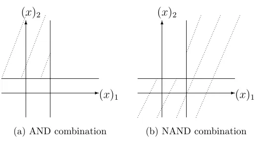
4.3 Kernels that Embed Combined Hypotheses . . . 50
4.3.1 Logic Kernels . . . 50
4.3.2 Multiplication of Logic Kernels . . . 51
4.3.3 Laplacian Kernel and Exponential Kernel . . . 55
4.3.4 Discussion on RBF Kernels . . . 58
5 Experiments 60 5.1 Setup . . . 60
5.2 Comparison of Ensemble Learning Algorithms . . . 62
5.2.1 Experimental Results . . . 62
5.2.2 Regularization and Sparsity . . . 63
5.3 Comparison of RBF Kernels . . . 65
List of Figures
1.1 Illustration of the learning scenario . . . 3
1.2 Overfitting and underfitting . . . 5
2.1 Illustration of the margin, where yi = 2·I[circle is empty]−1 . . . 15
2.2 The power of the feature mapping in (2.1) . . . 17
2.3 LPBoost can only choose one between h1 and h2 . . . 24
4.1 Illustration of the decision stump s+1,2,α(x) . . . 39
4.2 The XOR training set. . . 43
4.3 Illustration of the perceptron p+1,θ,α(x) . . . 46
4.4 Illustration of AND combination . . . 52
4.5 Combining s−1,1,2(x) and s+1,2,1(x) . . . 55
List of Tables
5.1 Details of the datasets . . . 61
5.2 Test error (%) comparison of ensemble learning algorithms . . . 63
5.3 Test error (%) comparison on sparsity and regularization . . . 65
5.4 Test error (%) comparison of RBF kernels . . . 66
List of Algorithms
Chapter 1
Introduction
This thesis is about infinite ensemble learning, a promising paradigm in machine learning. In this chapter, we would introduce the learning problem, the ensemble learning paradigm, and the infinite ensemble learning paradigm. We would build up our scheme of notations, and show our motivations for this work.
1.1
The Learning Problem
1.1.1
Formulation
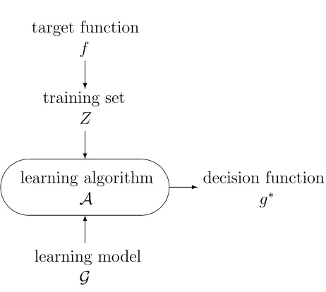
In this thesis, we would study the problem of learning from examples (Abu-Mostafa 1989). For such alearning problem, we are given atraining setZ ={zi: zi = (xi, yi)}Ni=1
which consists of the training examples zi. We assume that the training vectors xi
are drawn independently from an unknown probability measure PX(x) on X ⊆ RD,
and their labelsyi are computed from yi =f(xi). Here f: X → Y is called the target
function, and is also assumed to be unknown. With the given training set, we want to obtain a functiong∗:X → Y as our inference of the target function. The function
g∗ is usually chosen from a collection G of candidate functions, called the learning model. Briefly speaking, the task of the learning problem is to use the information in the training set Z to find some g∗ ∈ G that approximates f well.
problem, but we can also formulate it as a learning problem. We first ask someone to write down N digits, and represent their images by the training vectors xi. We then
label the digits byyi ∈ {0,1,· · · ,9}according to their meanings. The target function
f here encodes the process of our human-based recognition system. The task of this learning problem would be setting up an automatic recognition system (function)g∗
that is almost as good as our own recognition system, even on the yet unseen images of written digits in the future.
Throughout this thesis, we would work on binary classification problems, in which
Y ={−1,+1}. We call a function of the formX → {−1,+1} a classifier, and define the deviation between two classifiersg andf on a pointx∈ X to beI[g(x)6=f(x)].1
The overall deviation, called the out-of-sample error, would be
π(g) = Z
X
I[f(x)6=g(x)]dPX(x).
We say that g approximates f well, or generalizes well, ifπ(g) is small.
We design the learning algorithmA to solve the learning problem. Generally, the algorithm takes the training set Z and the learning modelG, and outputs a decision function g∗ ∈ G by minimizing a predefined error cost eZ(g). The full scenario of
learning is illustrated in Figure 1.1.
To obtain a decision function that generalizes well, we ideally desires eZ(g) = π(g)
for all g ∈ G. However, both f and pX are assumed to be unknown, and it is hence impossible to compute and minimizeπ(g) directly. A substitute quantity that depends only on Z is called the in-sample error
ν(g) =
N
X
i=1
I[yi 6=g(xi)]·
1 N .
Many learning algorithms consider ν(g) to be an important part of the error cost, because ν(g) is an unbiased estimate of π(g). The general wish is that a classifier g with a small ν(g) would also have a small π(g). Unfortunately, the wish does not
1I
target function f
?
training set Z
?
learning algorithm decision function
A g∗
'
&
$
%
-6
learning model
G
Figure 1.1: Illustration of the learning scenario
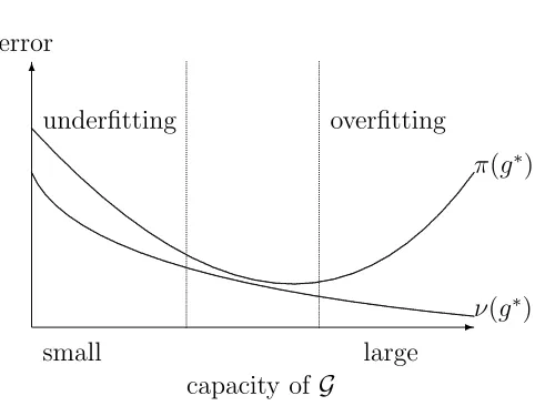
always come true. Although the in-sample error ν(g) is related to the out-of-sample error π(g) (Abu-Mostafa et al. 2004), a small ν(g) does not guarantee a small π(g) if the classifiers g ∈ G are considered altogether (Vapnik and Chervonenkis 1971). Next, we would show that the difference between π(g) and ν(g) could indicate how well the decision function g∗ generalizes.
1.1.2
Capacity of the Learning Model
It is known that the capacity of a learning model G plays an important role in the learning scenario (Cover 1965; Baum and Haussler 1989; Abu-Mostafa 1989; Vapnik 1998). The capacity of G denotes how the classifiers in G could classify different training sets (Cover 1965; Blumer et al. 1989). We say that G is more powerful, or more complex, if it has a larger capacity.
There are many approaches for measuring the capacity of a learning model (Cover 1965; Zhang 2002; Bousquet 2003; Vapnik 1998). One of the most important ap-proaches is the Vapnik-Chervonenkis dimension:
Definition 1 (Baum and Haussler 1989; Blumer et al. 1989) Consider the set of
{−1,+1}N, there exists g ∈ G such that yi =g(xi) for i= 1,2,· · · , N.
The Vapnik-Chervonenkis dimension (V-C dimension) of a learning model G,
de-noted DVC(G), is the maximum number N for which there exists X = {xi} N i=1 that
can be shattered by G. If there exists such X for all N ∈N, then DVC(G) =∞.
When G shatters a set of N training vectors {xi} N
i=1, we could find a classifier
g ∈ G that achieves ν(g) = 0 for any of the 2N possible labelings. In other words, G
is so powerful that no matter how those training labels are generated, we can always obtain zero in-sample error on this training set. The V-C dimension captures this classification power, or the capacity, by a single integer. Nevertheless, the integer is very informative in the learning theory (Baum and Haussler 1989; Abu-Mostafa 1989; Vapnik 1998). In particular, the difference between the out-of-sample and the in-sample error can typically be bounded by the V-C dimension.
Theorem 1 (Vapnik and Chervonenkis 1971; Abu-Mostafa 1989; Vapnik 1998) For
the binary classification problem, if the learning model G has DVC(G)<∞, then for
any >0, there exists some N0 ∈N such that for any training set of size N ≥N0,
Pr
sup
g∈G
π(g)−ν(g) >
≤4 (2N)DVC(G)+ 1exp
−N
2
8
(1.1)
Theorem 1 is a route to estimate the out-of-sample error from the in-sample error. The inequality (1.1) is independent ofpX andf. In addition, it is a worst-case bound for all g ∈ G, and thus can also be applied to the decision function g∗. Next, we
use this theorem to explain how the choice of a suitable G affects the generalization performance ofg∗.
6
-capacity of G
small large
Figure 1.2: Overfitting and underfitting
even if we obtain a decision function g∗ with a small ν(g∗), the function may still
have a large π(g∗).
On the other hand, we can use a learning model G with a very small capacity to avoid overfitting. Then, the bound in (1.1) would be smaller. However, if allg ∈ Gare too simple, they could be very different from the target function f. In other words, bothν(g) and π(g) would be large for all g ∈ G. Hence, the learning algorithm could not output any g∗ that has a small π(g∗). This situation is called underfitting.
We illustrate the typical behavior of overfitting and underfitting in Figure 1.2. Successful learning algorithms usually handle these situations by working implicitly or explicitly with a reasonable learning model. One famous strategy, called regular-ization, implicitly shrinks the capacity ofG by only considering some simpler subsets of G, or by penalizing the more complex subsets of G. Regularization helps to avoid overfitting, and is inherit in many learning algorithms, such as the Support Vector Machine that we would encounter later.
a remedy to underfitting. We would further explore the use of regularization and boosting in this thesis.
1.2
Ensemble Learning
1.2.1
Formulation
The ensemble learning paradigm denotes a large class of learning algorithms (Meir and R¨atsch 2003). Instead of considering a powerful learning model G, an ensemble learning algorithm A deals with a base learning model H, which is usually simple. The classifiers h∈ Hare often calledhypothesesorbase learners. The algorithm then constructs a decision function g∗ by 2
g∗(x) = sign
T
X
t=1
wtht(x)
! ,
wt ≥0, t= 1,2,· · · , T.
(1.2)
Any classifier g∗ that could be expressed by (1.2) is called an ensemble classifier, and
thewt in (1.2) are called thehypothesis weights. Without lose of generality for possible
ensemble classifiers, we usually normalizewbyPT
t=1wt. Then the hypothesis weights
would sum to 1.3 For each ensemble classifier in (1.2), we can define its normalized
version as
g∗(x) = sign
T
X
t=1
˜ wtht(x)
! ,
T
X
t=1
˜
wt = 1,w˜t ≥0, t= 1,2,· · ·, T.
(1.3)
We would denote the normalized hypothesis weights by ˜w, while reserving w for pos-sibly unnormalized ones. Note that ˜w and w can usually be used interchangeably, because scaling the hypothesis weights by a positive constant does not affect the
2
sign(v) is 1 when vis nonnegative,−1 otherwise.
3
prediction after the sign(·) operation. By considering normalized classifiers, we can see that that g∗ ∈ cvx(H), where cvx(H) means the convex hull of H in the
func-tion space. In other words, the ensemble learning algorithm A actually works on
G = cvx(H).
AlthoughH could be of infinite size in theory, traditional ensemble learning algo-rithms usually deal with a finite and predefined T in (1.2). We call these algorithms
finite ensemble learning. Finite ensemble learning algorithms usually share another common feature: they choose each hypothesis ht by calling another learning
algo-rithm AH, called the base learning algorithm.
Another approach in ensemble learning is infinite ensemble learning, in which the size of {ht} is not finite. For infinite ensemble learning, the set {ht} could either
be countable or uncountable. In the latter situation, a suitable integration would be used instead of the summation in (1.2).
Successful ensemble learning algorithms include Bayesian Committee Machines (Tresp 2000), Bootstrap Aggregating (Breiman 1996), Adaptive Boosting (Freund and Schapire 1997), and Adaptive Resampling and Combining (Breiman 1998). In a broad sense, Bayesian inference that averages the predictions over the posterior probability also belongs to the ensemble learning family (Vapnik 1998).
1.2.2
Why Ensemble Learning?
Ensemble learning algorithms are often favorable for having some or all of the follow-ing three properties: stability, accuracy, and efficiency (Meir and R¨atsch 2003).
1. Stability:
If a learning algorithm outputs a very different decision functiong∗ when there
is a small variation in Z, we call the algorithm unstable. Unstable learning algorithms are often not desirable, because they are easily affected by noise, imprecise measurements, or even numerical errors in computing. Such algo-rithms also may not output some g∗ that generalize well, because of the large
The stability of ensemble learning algorithms is best illustrated by theBootstrap Aggregating(Bagging) algorithm (Breiman 1996). Bagging generatesT training sets Z(t) by bootstrapping Z, and applies the base learning algorithm A
H on
eachZ(t)to obtainh
t. The majority vote of eachht(x) determines the prediction
for some x ∈ X. In other words, the normalized hypothesis weights ˜wt are
always set to T1 in (1.3). Breiman (1996) shows that the Bagging algorithm A
is stabler than the base learning algorithm AH because of the voting strategy. Thus, we can view the ensemble learning algorithm as an approach to make the base learning algorithm stabler.
2. Accuracy:
The ensemble learning algorithm usually outputs a decision functiong∗ that has
a smaller π(g∗) than each individual π(h
t). One simple explanation is that a
voting approach like Bagging could eliminate uncorrelated errors made by each classifier ht. A deeper justification comes from the Probably Approximately
Correct (PAC) theory of learnability (Valiant 1984). In particular, when the size of the training set is large enough, even if each classifierhtperforms only slightly
better than random guess tof, we would construct an ensemble classifierg∗that
is very close to f (Kearns and Valiant 1994). The boosting strategy illustrated in Section 1.1 gets its name because of this theoretical result.
3. Efficiency:
the Adaptive Boosting algorithm (see Section 2.2) could perform a complicated search in G with only some small number of calls to AH.
1.3
Infinite Ensemble Learning
We have introduced the basics of ensemble learning. In this section, we would discuss the motivations and possible difficulties for infinite ensemble learning.
1.3.1
Why Infinite Ensemble Learning?
The most important reason for going from finite ensemble learning to infinite ensemble learning is to further increase the capacity of the learning model. Baum and Haussler (1989) show that ensemble classifiers in (1.2) with a finite predefined T is limited in power.
Theorem 2 (Baum and Haussler 1989) For a base learning model H and a finite
predefined T ≥2, let
G ={g: g can be represented by (1.2) with ht ∈ H for all t= 1,2,· · · , T}.
Then, DVC(G)≤4T log2(eT).
Thus, choosing a suitableT for finite ensemble learning is as important as choosing a suitable G for a learning algorithm. On the one hand, the limit in capacity could make the algorithm less vulnerable to overfitting (Rosset et al. 2004). On the other hand, the limit raises a possibility of underfitting (Freund and Schapire 1997).
harm-ful to go closer to infinity by enlarging T (R¨atsch et al. 2001). The controversial results suggest further research on infinite ensemble learning.
There are many successful learning algorithms that work well by combining in-finite processes, transition probabilities, or features. For example, inin-finite Gaussian Mixture Model (Rasmussen 2000), infinite Hidden Markov Model (Beal et al. 2003), or Support Vector Machine (Vapnik 1998). They successfully demonstrate that it can be beneficial to consider infinite mixtures in the learning model. Thus, we want to study whether infinite ensemble learning, that is, an infinite mixture of hypotheses, could also work well. In particular, our motivation comes from an open problem of Vapnik (1998, page 704):
The challenge is to develop methods that will allow us to average over large (even
infinite) numbers of decision rules using margin control. In other words, the problem
is to develop efficient methods for constructing averaging hyperplanes in high
dimen-sional space.
Here the “decision rules” are the hypotheses in H, the “margin control” is for performing regularization, and the “averaging hyperplane” is the ensemble classifier. Briefly speaking, our task is to construct an ensemble classifier with an infinite number of hypotheses, while implicitly controlling the capacity of the learning model. Next, we will see the difficulties that arise with this task.
1.3.2
Dealing with Infinity
To perform infinite ensemble learning, we would want to check and output classifiers of the form
g(x) = sign
∞
X
t=1
wtht(x)
! ,
or in the uncountable case,
g(x) = sign Z
α∈C
wαhα(x)dα
, wα ≥0, α∈ C.
The countable and uncountable cases share similar difficulties. We would conquer both cases in this thesis. Here, we will only discuss the countable case for simplicity. The first obstacle is to represent the classifiers. The representation is important both for the learning algorithm, and for doing further prediction with the decision function g∗. We cannot afford to save and process every pair of (w
t, ht) because of
the infinity. One approach is to save only the pairs with nonzero hypothesis weights, because the zero weights do not affect the predictions of any ensemble classifier g. We call this approach sparse representation.
An ensemble classifier that only has a small finite number of nonzero hypothesis weights is called a sparse ensemble classifier. The viability of sparse representation is based on the assumption that the learning algorithm only needs to handle sparse ensemble classifiers. Some algorithms could achieve this assumption by applying an error cost eZ(g) that favors sparse ensemble classifiers. An example of such design
is the Linear Programming Boosting algorithm (Demiriz et al. 2002), which would be introduced in Section 2.2. The assumption on sparse ensemble classifiers is also crucial to many finite ensemble learning algorithms, because such property allows them to approximate the solutions well with a finite ensemble.
With the sparse representation approach, it looks as if infinite ensemble learning could be solved or approximated by finite ensemble learning. However, the sparsity assumption also means that the capacity of the classifiers is effectively limited by Theorem 2. In addition, it is not clear whether the error cost eZ(g) that introduces
sparsity could output a decision function g∗ that generalizes well. Thus, we choose
Another obstacle in infinite ensemble learning is the infinite number of constraints
wt ≥0, t= 1,2,· · · ,∞.
Learning algorithms usually try to minimize the error cost eZ(g), which becomes a
harder task when more constraints needs to be satisfied and maintained simultane-ously. The infinite number of constraints resides in the extreme of this difficulty, and is part of the challenge mentioned by Vapnik (1998).
1.4
Overview
This thesis exploits the Support Vector Machine (SVM) to tackle the difficulties in infinite ensemble learning. We would show the similarity between SVM and boosting-type ensemble learning algorithms, and formulate an infinite ensemble learning frame-work. based on SVM. The key of the framework is to embed infinite number of hy-potheses into the kernel of SVM. Such framework does not require the assumption for sparse representation, and inherits the profound theoretical results of SVM.
We find that we can apply this framework to construct new kernels for SVM, and to interpret some existing kernels. In addition, we can use this framework to fairly compare SVM with other ensemble learning algorithms. Experimental results show that our SVM-based infinite ensemble learning algorithm has superior performance over popular ensemble learning algorithms.
Chapter 2
Connection between SVM and
Ensemble Learning
In this chapter, we focus on connecting Support Vector Machine (SVM) to ensemble learning algorithms. The connection is our first step towards designing an infinite ensemble learning algorithm with SVM. We start by providing the formulations of SVM in Section 2.1, and show that SVM implements the concept of large-margin classifiers. Next in Section 2.2, we introduce some ensemble learning algorithms that also output large-margin classifiers. Then, we would further discuss the connection between SVM and those algorithms in Section 2.3.
2.1
Support Vector Machine
2.1.1
Basic SVM Formulation
We start from a basic SVM formulation: linear hard-margin SVM (Vapnik 1998), which constructs a decision function 1
g∗(x) = sign wTx+b
with the optimal solution (w, b) to the following problem:
(P1) max
w∈RD,b∈R,ρ∈RN 1min≤i≤Nρi
subject to ρi =
1
kwk2yi w
Tx i +b
, i= 1,2,· · · , N,
ρi ≥0, i= 1,2,· · · , N.
The classifier of the form sign wTx+b
is called ahyperplane classifier, which divides the space RD with the hyperplane wTx+b = 0. For a given hyperplane classifier,
the value ρi is called the `2-margin of each training example zi = (xi, yi), and its
magnitude represents the Euclidean distance of xi to the hyperplane wTx+b = 0.
We illustrate the concept of margin in Figure 2.1. The constraint ρi ≥0 means that
the associated training example zi is classified correctly using the classifier. Linear
hard-margin SVM would output a hyperplane classifier that not only classifies all training examples correctly (called separates all training examples), but also has the largest minimum margin. In other words, the distance from any training vector to the hyperplane should be as large as possible.
The intuition for obtaining a large-margin classifier is to have less uncertainty near the decision boundary wTx+b = 0, where sign(·) switches sharply. A deeper
theoretical justification is that the large-margin concept implicitly limits the capacity of the admissible learning model.
Theorem 3 (Vapnik 1998) Let the vectors x ∈ X ⊆ RD belong to a sphere of
ra-1
Here uT means the transpose of the vectoru, and hence uTv is the inner product of the two
dx1
Figure 2.1: Illustration of the margin, where yi = 2·I[circle is empty]−1
dius R, and define the Γ-margin hyperplane
gw,b(x) =
Then, the learning modelG that consists of all theΓ-margin hyperplanes has V-C di-mension
Thus, when choosing the hyperplane with the largest minimum margin, we could shrink and bound the capacity of the learning model. As mentioned in Section 1.1, this idea corresponds to the regularization strategy for designing learning algorithms. Problem (P1) contains the max-min operation and nonlinear constraints, which
are complicated to solve. Nevertheless, the optimal solution (w, b) for a following simple quadratic problem is also optimal for (P1).
The quadratic problem (P2) is convex and is easier to analyze. In the next section,
we would construct more powerful SVM formulations based on this problem.
2.1.2
Nonlinear Soft-Margin SVM Formulation
Linear hard-margin SVM problem (P2) has a drawback: what if the training examples
cannot be perfectly separated with any hyperplane classifier? Figure 2.2(a) shows a training set of such situation. Then, the feasible region of (P2) would be empty, and
the algorithm could not output any decision function (Lin 2001).
This situation happens because the learning model (set of hyperplane classifiers) is not powerful enough, or because the training examples contain noise. Nonlinear soft-margin SVM applies two techniques to deal with the situation. First, it uses the feature transformation to increase the capacity of the learning model. Second, it al-lows the hyperplane classifier to violate some of the the constraints of (P2) (Sch¨olkopf
and Smola 2002).
Nonlinear SVM works in a feature spaceF rather than the original spaceX ⊆RD.
The original vectorsx∈ X are transformed to the feature vectorsφx ∈ F by afeature
mapping
Φ : X → F
x7→φx .
We assume that the feature space F is a Hilbert space defined with an inner prod-uct h·,·i. Then, we can replace the wTx in linear SVM by hw, φ
xi. The resulting
classifier would still be of hyperplane-type in F, and hence Theorem 3 could be ap-plied by considering φx instead ofx. When Φ is a complicated feature transform, it is
likely that we could separate the training examples in F. For example, assume that
Φ : R2 → F =R5
(x)1,(x)2
7→
(x)1,(x)2,(x)21,(x)1(x)2,(x)22
,
d
t t
d
(a) No hyperplane classifier could separate the training examples
d
(b) A quadratic curve classifier separates the training examples
Figure 2.2: The power of the feature mapping in (2.1)
where (x)d is the d-th element of the vector x. Then, any classifier of the form
sign
hw,Φ(x)i+b
would be a quadratic curve inR2, and the set of such classifiers is more powerful than
the set of hyperplane classifiers inR2, as illustrated by Figure 2.2.
With a suitable feature transform, nonlinear soft-margin SVM outputs the deci-sion function
with the optimal solution to
(P3) min
The valueξi is the violation that the hyperplane classifier makes on training examples
zi = (xi, yi), and C > 0 is the parameter that controls the amount of the total
violations allowed. WhenC → ∞, we call (P3) the problem ofnonlinear hard-margin
Because the feature space F could be of infinite number of dimensions, SVM software usually solves the Lagrangian dual of (P3) instead:
(P4) min
Here K is called the kernel, and is defined as
K(x, x0)≡ hφx, φx0i. (2.3)
The duality between (P3) and (P4) holds for any Hilbert spaceF (Lin 2001). Through
duality, the optimal (w, b) for (P3) and the optimal λ for (P4) are related by (Vapnik
1998; Sch¨olkopf and Smola 2002)
w=
Then, the decision function becomes
g∗(x) = sign
An important observation is that both (P4) and (2.6) do not require any
dimensions, we could solve (P4) and obtain g∗ with only the kernelK(x, x0). The use
of a kernel instead of directly computing the inner product in F is called the kernel trick, and is a key ingredient of SVM.
For the kernel trick to go through, the kernelK(x, x0) should be easy to compute.
Alternatively, we may wonder if we could start with an arbitrary kernel, and claim that it is an inner producth·,·iin some space F. An important tool for this approach is the Mercer’s condition. Next, we first define some important terms in Definition 2, and describe the Mercer’s condition briefly in Theorem 4.
Definition 2 For some N byN matrix K,
1. K is positive semi-definite (PSD) if vTKv≥0 for all v ∈RN.
2. K is positive definite (PD) if vTKv > 0 for all v ∈ RN such that some v i is
nonzero.
3. K is conditionally positive semi-definite (CPSD) if vTKv ≥ 0 for all v ∈ RN
such that PN
i=1vi = 0.
4. K is conditionally positive definite (CPD) if vTKv >0for all v ∈RN such that
PN
i=1vi = 0and some vi is nonzero.
Theorem 4 (Vapnik 1998; Sch¨olkopf and Smola 2002) A symmetric functionK(x, x0) is a valid inner product in some spaceF if and only if for every N and{xi}Ni=1 ∈ XN,
the matrix K constructed by Kij =K(xi, xj), called the Gram matrix of K, is PSD.
Several functions are known to satisfy Mercer’s condition for X ⊆RD, including:
• Linear: K(x, x0) = xTx0.
• Polynomial: K(x, x0) = (xTx0 +r)k, r≥ 0, k ∈N.
• Gaussian: K(x, x0) = exp −γkx−x0k2 2
, γ >0.
• Exponential: K(x, x0) = exp (−γkx−x0k
• Laplacian: K(x, x0) = exp (−γkx−x0k
1), γ >0.
SVM with different kernels try to classify the examples with large-margin hyper-plane classifiers in different Hilbert spaces. Some ensemble learning algorithms can also produce large-margin classifiers with a suitable definition of the “margin.” Note that we deliberately use the same symbol win (P3) for the hyperplane classifiers and
for the hypothesis weights in ensemble learning. In the next section, we shall see that this notation easily connects SVM to ensemble learning through the large-margin concept.
2.2
Ensemble Learning and Large-Margin Concept
We have introduced SVM and the large-margin concept. In this section we show two ensemble learning algorithms that also output large-margin classifiers. The first one is Adaptive Boosting, and the second one is Linear Programming Boosting.
2.2.1
Adaptive Boosting
Adaptive Boosting (AdaBoost) is one of the most popular algorithms for ensemble learning (Freund and Schapire 1996; Freund and Schapire 1997). For a given inte-ger T, AdaBoost iteratively forms an ensemble classifier
g∗(x) = sign
T
X
t=1
wtht(x)
!
, wt ≥0, t = 1,2,· · ·, T.
In each iteration t, there is a sample weight Ut(i) on each training example zi, and
AdaBoost selects ht ∈ H with the least weighted in-sample error:
ht = argminh∈H N
X
i=1
I[yi 6=h(xi)]·Ut(i)
! .
AdaBoost then assigns the unnormalized hypothesis weight wt to ht, and generates
Algorithm 1 has an interpretation as a gradient-based optimization technique (Mason et al. 2000). It obtains the hypotheses and weights by solving the following optimization problem:
(P5) max
wt∈R,ht∈H,ρ∈RN −
N
X
i=1
exp (− kwk1ρi)
subject to ρi =
1
kwk1yi
∞
X
t=1
wtht(xi)
!
, i= 1,2,· · ·, N,
wt ≥0, t= 1,2,· · · ,∞.
Although (P5) has an infinite number of variables (wt, ht), AdaBoost approximates
the optimal solution by the first T steps of the gradient-descent search. We could compare (P5) with (P1). First, they have a similar term ρi. However, for SVM, ρi
is the `2-margin, while for AdaBoost, ρi is normalized by kwk1, and is called the
`1-margin. The objective function of SVM is
min
1≤i≤N ρi,
while the objective function of AdaBoost is
N
X
i=1
−exp (− kwk1ρi).
For large ρi, the term exp (− kwk1ρi) would be close to zero and negligible. Thus,
the two objective functions both focus only on smallρi. Note that for a fixed w, the
term
−exp (− kwk1ρi)
is an increasing function ofρi. Thus, both (P5) and (P1) want to maximize the smaller
margins.
In other words, AdaBoost asymptotically approximates an infinite ensemble classifier
g∗(x) = sign
∞
X
t=1
wtht(x)
! ,
such that (w, h) is an optimal solution for
(P6) min
wt∈R,ht∈H
kwk1
subject to yi
∞
X
t=1
wtht(xi)
!
≥1, i= 1,2,· · · , N.
wt ≥0, t= 1,2,· · ·,∞. (2.7)
Compare (P6) with (P3), we further see the similarity between SVM and AdaBoost.
Note, however, that AdaBoost has additional constraints (2.7), which makes the problem harder to solve directly.
2.2.2
Linear Programming Boosting
Linear Programming Boosting (LPBoost) solves (P6) exactly with linear
program-ming. We will introduce soft-margin LPBoost, which constructs an infinite ensemble classifier
g∗(x) = sign
∞
X
t=1
wtht(x)
! ,
with the optimal solution to
(P7) min
wt∈R,ht∈H ∞
X
t=1
wt +C N
X
i=1
ξi
subject to yi
∞
X
t=1
wtht(xi)
!
≥1−ξi,
ξi ≥0, i= 1,2,· · · , N,
Similar to the case of soft-margin SVM, the parameter C controls the amount of violations allowed. When C → ∞, the soft-margin LPBoost approaches a hard-margin one, which solves (P6) to obtain the decision function g∗.
LPBoost is an infinite ensemble learning algorithm. How does it handle infinite number of variables and constraints? First, there are many optimal solutions to (P7),
and some of them only have a finite number of nonzero hypothesis weights wt. For
example, consider two hypothesis ht1 and ht2 such that
ht1(xi) =ht2(xi) for i= 1,2,· · · , N.
We say that ht1 and ht2 have the same pattern, or are ambiguous, on the training
vectors {xi}Ni=1. Assume that (w, h) is an optimal solution for (P7), and define
ˆ wt =
wt1 +wt2 t=t1
0 t=t2
wt otherwise.
Then, we can see that ( ˆw, h) satisfies all the constraints of (P7), and still has the same
objective value as (w, h). Thus, ( ˆw, h) is also an optimal solution. We can repeat this process and get an optimal solution that has at most 2N nonzero weights. LPBoost
aims at finding this solution. Thus, it equivalently only needs to construct a finite ensemble classifier of at most 2N hypothesis weights.
Even if LPBoost would need at most 2N nonzero hypothesis weightsw
t, the
prob-lem could still be intractable when N is large. However, minimizing the criteria kwk1
often produces a sparse solution (Meir and R¨atsch 2003; Rosset et al. 2004). Hence, LPBoost could start with all zero hypothesis weights, and iteratively considers one hypothesis ht that should have non-zero weightwt. Because (P7) is a linear
program-ming problem, such step can be performed efficiently with a simplex-type solver using the column generation technique (Nash and Sofer 1996). The detail of LPBoost is shown in Algorithm 2.
d d
d d
d
@ @
@ @
@ @
@ @
@ @
@ @
@ @
@ @
h1
h2
t t
t
t t
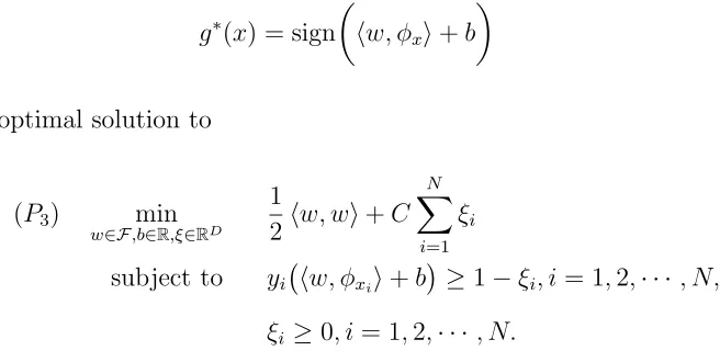
Figure 2.3: LPBoost can only choose one between h1 and h2
could be slow. As a consequence, the assumption on sparse representation becomes important, because the level of sparsity determines the number of inner optimization problems that LPBoost needs to solve. Second, for any specific pattern on the training vectors, LPBoost use one and only one ht to represent it. The drawback here is that
the single hypothesisht may not be the best compared to other ambiguous hypotheses.
Figure 2.3 shows one such situation, in which the hypotheses are hyperplanes in two dimensional spaces. The classifier h1 seems to be a stabler choice over h2 for the
pattern, but LPBoost might only select h2 as the representative. This drawback
contradicts the ensemble view for stability: we should average over the predictions of the ambiguous hypotheses to obtain a stabler classifier.
2.3
Connecting SVM to Ensemble Learning
In (P7), we consider selecting an infinite number of hypotheses ht from H, and then
assigning the hypothesis weights wt to them. When H is of countably infinite size,
an equivalent approach is to assumeH ={h(a)}∞a=1, and obtain a nonnegative weight
and a as a general enumeration. Consider the feature transform
Φ(x) = (h(1)(x), h(2)(x),· · · , h(a)(x),· · ·). (2.8)
From (P3) and (P7), we can clearly see the connection between SVM and LPBoost.
The features in φx in SVM and the hypotheses h(a)(x) in LPBoost play similar roles.
SVM and LPBoost both work on linear combinations of the features (hypothesis predictions), though SVM has an additional intercept term b. They both minimize the sum of a margin-control term and a violation term. However, SVM focuses on the `2-margin while LPBoost deals with the `1-margin. The later results in sparse
representation of the ensemble classifier.
The connection between SVM and ensemble learning is widely known in literature. Freund and Schapire (1999) have shown the similarity of large-margin concept be-tween SVM and AdaBoost. The connection has been used to develop new algorithms. For example, R¨atsch et al. (2001) have tried to select the hypotheses by AdaBoost and obtain the hypothesis weights by solving an optimization problem similar to (P3).
Another work by R¨atsch et al. (2002) has shown a new one-class estimation algorithm based on the connection. Recently, Rosset et al. (2004) have applied the similarity to compare SVM with boosting algorithms.
Although H can be of infinite size, previous results that utilize the connection between SVM and ensemble learning usually only consider a finite subset ofH. One of the reasons is that the constraints w(a) ≥ 0, which are required for ensemble
learning, are hard to handle in SVM. If we have an infinite number of hypothesis weights, and directly add the nonnegative constraints to (P3), Vapnik (1998) shows
that the dual problem (P4) would become
(P8) min
λ∈RN,ζ
1 2
N
X
i=1
N
X
j=1
λiλjyiyjK(xi, xj)− N
X
i=1
λi+ N
X
i=1
yiλihφxi, ζi+
1 2hζ, ζi subject to 0≤λi ≤C, i= 1,· · · , N,
Because ζ is an unknown vector of infinite size, we cannot perform h·, ζi with the kernel trick. In addition, we still have an infinite number of variables and constraints in (P8), and we cannot solve such problem directly. We would deal with these
Algorithm 1 AdaBoost
• Input:
– The training set Z ={(x1, y1), ...,(xN, yN)}.
– The number of iterations T.
– The base learning model H and the base learning algorithm AH.
• Procedure:
– Initialize the sample weights U1(i) = 1/N for i= 1,2,· · · , N.
– For t= 1,· · ·, T do
1. Call AH to obtain ht ∈ H that achieves the minimum error on the
weighted training set (Z, Ut).
2. Calculate the weighted errort of ht.
t = N
X
i=1
I[ht(xi)6=yi]·Ut(i),
Abort if t = 0 ort ≥ 12.
3. Set
wt = log
1−t
t
, and update the sample weights by
Ut+1(i) =Ut(i) exp (−wtI[ht(xi) =yi]), for i= 1,2,· · · , N.
4. Normalize Ut+1 such that PNi=1Ut+1(i) = 1.
• Output:
– The decision function g∗(x) = signPT
t=1wtht(x)
Algorithm 2 LPBoost
• Input:
– The training set Z ={(x1, y1), ...,(xN, yN)}.
– The soft-margin parameter C.
– The base learning model H and the base learning algorithm AH.
• Procedure:
– Initialize the sample weights U1(i) = 1/N for i= 1,2,· · · , N.
– Initialize β1 = 0.
– For t= 1,· · ·,∞ do
1. Call AH to obtain ht ∈ H that achieves the minimum error on the
weighted training set (Z, Ut).
2. Check if ht could really improve the optimal solution:
If PN
i=1Ut(i)yiht(xi)≤βt, T ←t−1, break.
3. Update the sample weights Ut and current optimality barrier βt by
solving
(P9) min
Ut+1,βt+1
βt+1
subject to
N
X
i=1
Ut+1(i)yihk(xi)≤βt+1, k= 1,· · · , t, (2.9)
N
X
i=1
Ut+1(i) = 1,
0≤Ut+1(i)≤C, i= 1,· · · , N.
4. Update the weight vector w with the Lagrange multipliers of (2.9).
• Output:
– The decision function g∗(x) = signPT
t=1wtht(x)
Chapter 3
SVM-based Framework for Infinite
Ensemble Learning
Our goal is to conquer the task of infinite ensemble learning without confining our-selves to the sparse representation. Traditional algorithms cannot be directly general-ized to solve this problem, because they either iteratively include only a finite number of T hypotheses (AdaBoost), or assume sparse representation strongly (LPBoost).
The connection between SVM and ensemble learning shows another possible ap-proach. We can form a kernel that embodies the predictions of all the hypotheses in H. Then, the decision function (2.6) obtained from SVM with this kernel is a linear combination of those predictions (with an intercept term). However, there are still two main obstacles. One is to compute the kernel when H is of possibly un-countable size, and the other is to handle the nonnegative constraints on the weights to make (2.6) an ensemble classifier. In this chapter, we shall address the details of these obstacles, and then propose a thorough framework that exploits SVM for infinite ensemble learning.
3.1
Embedding Learning Model into the Kernel
In this section, we try to embed the hypotheses in the base learning modelH into an SVM kernel. Our goal is infinite ensemble learning. Thus, although the embedding works when H is of either finite or infinite size, we would assume the infinite case.
predictions of the hypothesesh(a) ∈ H. In Definition 3, we extend this idea to a more
general form, and defines a kernel based on the feature mapping.
Definition 3 Assume that H ={hα:α ∈ C}, where C is a measure space with
mea-sure µ. The kernel that embodies H with a positive function r: C → R+ is defined
as
KH,r(x, x0) =
Z
C
φx(α)φx0(α)dµ(α), (3.1)
whereφx(α) =r(α)hα(x)is a measurable function overµ, and the embedding function
r(α) is chosen such that the Lebesgue integral exists for all x, x0 ∈ X.
Here, the indexα is called theparameter of the hypothesishα. Note that
depend-ing on the way that we parameterize H, two hypotheses hα1 and hα2, where α1 6=α2,
may have hα1(x) =hα2(x) for all x∈ X. For example, we could parameterize the set
of finite ensemble classifiers in (1.2) by (w, h). But an ensemble classifier with param-eter (w, h) is equivalent to an ensemble classifier with paramparam-eter ( ˜w, h), where ˜wt are
the associated normalized hypothesis weights. We would treat those hypotheses as different objects during parameterization, while bearing in mind that they represent the same function. That is, the learning model H is equivalently S
α∈C{hα}.
From now on, we shall denote KH,r by KH when it is clear about the embedding
function r from the context, or when the specific choice of r is irrelevant. If C is a closed interval [L, R], we can easily observe that the right-hand-side of (3.1) is an inner product (Sch¨olkopf and Smola 2002), and hence Definition 3 constructs a valid kernel. In the following theorem, we formalize such observation for a general C.
Theorem 5 Consider the kernel KH =KH,r in Definition 3.
1. The kernel is an inner product forφxandφx0 in the Hilbert spaceF =L2(C, dµ), where L2(C, dµ) is the set of functions ϕ(·) : C → R that are square integrable
over measure µ.
2. For a given set of training vectors X ={xi}Ni=1 ∈ XN, the Gram matrix of KH
Proof. By Definition 3,
KH,r(x, x) =
Z
C
(φx(α))2 dµ(α)
exists for allx∈ X. Thus, the functions φx(α) belongs toF =L2(C, dµ). The results
of Reed and Simon (1980, Section II.2, Example 6) show that F is a Hilbert space, in which the inner product between two functions ϕand ϕ0 is defined as
hϕ, ϕ0i=
Z
C
ϕ(α)ϕ0(α)dµ(α).
Then, we can see that KH(x, x0) is an inner product forφx and φx0 inF. The second
part is just a consequence of the first part by Theorem 4.
The technique for using an integral inner product between functions is known in SVM literature. For example, Sch¨olkopf and Smola (2002, Section 13.4.2) explain that the Fisher kernel takes an integral inner product between two regularized functions. Our framework applies this technique to combine predictions of hypotheses, and thus could handle the situation even when the base learning model H is uncountable. When we apply KH to (P4), the primal problem (P3) becomes
(P10) min
w,b,ξ
1 2
Z
C
(w(α))2 dµ(α) +C
N
X
i=1
ξi
s.t. yi
Z
C
w(α)r(α)hα(xi)dµ(α) +b
≥1−ξi,
ξi ≥0, i= 1,· · · , N,
w ∈ L2(C, dµ), b∈R, ξ∈RN.
In particular, the decision function (2.6) obtained after solving (P4) with KH is the
same as the decision function obtained after solving (P10):
g∗(x) = sign Z
C
w(α)r(α)hα(x)dµ(α) +b
. (3.2)
infinitesimal weight w(α)r(α)dµ(α) in g∗(x). We shall discuss this situation further
in Section 3.3. Note that (3.2) is not an ensemble classifier yet, because we do not have the constraints w(α) ≥ 0 for all possible α ∈ C, and we have an additional intercept term b.1 In the next section, we focus on these issues, and explain that
g∗(x) is equivalent to an ensemble classifier under some reasonable assumptions.
3.2
Assuming Negation Completeness
To make (3.2) an ensemble classifier, we need to have w(α) ≥ 0 for all α ∈ C. Somehow these constraints are not easy to satisfy. We have shown in Section 2.3 that even when we only add countably infinite number of constraints to (P3), we would
introduce infinitely many variables and constraints in (P8), which makes the later
problem difficult to solve (Vapnik 1998).
One remedy is to assume that H is negation complete, that is,2
h ∈ H ⇔(−h)∈ H.
Then, every linear combination over H has an equivalent linear combination with only nonnegative hypothesis weights. Thus, we can drop the constraints during op-timization, but still obtain a decision function that is equivalent to some ensemble classifier. For example, forH={h1, h2,(−h1),(−h2)}, if we have a decision function
sign(3h1(x)−2h2(x)),
it is equivalent to
sign(3h1(x) + 2(−h2)(x)),
and the later is an ensemble classifier over H. 1
Actually,w(α)r(α)≥0. Somehow we assumed thatr(α) is always positive.
2
Algorithm 3 SVM-based framework for infinite ensemble learning
• Input:
– The training set Z ={(x1, y1),· · · ,(xN, yN)}.
– The soft-margin parameter C.
– The base learning model H and the kernel KH given in Definition 3. The kernel is computed from H, which is assumed to be an infinite, negation complete learning model that contains a constant classifier.
• Procedure:
– Solve (P4) withKH and obtain Lagrange multipliers λi.
– Compute b from (2.5).
• Output:
– The decision function g∗(x) = signPN
i=1yiλiK(xi, x) +b
, which is equiv-alent to some ensemble classifier over H.
Note that negation completeness is usually a mild assumption for a reasonable learning model. Following this assumption, after solving (P4) with KH, the decision
function (3.2) can be interpreted an ensemble classifier overHwith an intercept term b. Note that b can be viewed as a hypothesis weight on a constant classifier c, which predicts c(x) = 1 for all x ∈ X. In general, a reasonable learning model H contains cand (−c), in order to handle, for example, the situation that all training labels are the same. We shall make the assumption thatH contains both cand (−c) from now on. Then, g∗(·) in (3.2) or (2.6) is indeed equivalent to an ensemble classifier.
3.3
Properties of the Framework
In this section, we introduce two important properties of the SVM-based framework. First we show that the framework allows us to embed multiple base learning models together with a simple summation over the kernels. This property demonstrates not only an advantage of the framework, but also the simpicity of manipulating with kernels. Second, we show that the framework treats the ambiguous hypotheses fairly. We have mentioned in Section 2.2 that LPBoost could only select one hypothesis among the ambiguous ones, but our framework would average over the predictions of all of them. Thus, from the ensemble point-of-view, our framework would be stabler.
3.3.1
Embedding Multiple Learning Models
The SVM-based framework allows us to embed multiple base learning models alto-gether. Consider two base learning models H1 and H2, if we could embed them into
kernels KH1 and KH2, respectively, then the kernel
K(x, x0) =KH1(x, x0) +KH2(x, x0)
embeds both of those learning models. In other words, if we use K(x, x0) in
Algo-rithm 3, and H = H1 ∪ H2 satisfies the required assumptions, we could obtain an
ensemble classifier over H.
When we want to consider multiple base learning models together, traditional ensemble learning algorithms usually require calling a base learning algorithm for each model. Such step is usually more time-consuming than just summing up the kernel evaluations. In fact, as shown in the next theorem, our framework could embed a countably infinite number of base learning models altogether, which can hardly be done by traditional ensemble learning algorithms.
KH1,· · · ,KHM with learning modelsH1,· · · ,HM, respectively. Then, let
K(x, x0) =
M
X
m=1
KHm(x, x0).
If K(x, x0) exists for all x, x0 ∈ X, and
H=
M
[
m=1
Hm∪ {c,(−c)}
is negation complete, Algorithm 3 using K(x, x0) could output an ensemble classifier over H.
Proof. From Theorem 5, eachKHm is an inner product in a Hilbert space Fm. From
the results of Reed and Simon (1980, Example 5), we can see that a countable direct sum over Hilbert spaces is still a Hilbert space. Let F be the countable direct sum of the spaces F1,· · · ,FM, we could define an inner product in F by summing the
inner products inF1,· · · ,FM. The resulting inner product isK(x, x0), and hence the
decision function g∗ from (3.2) represents a linear combination over the predictions
of SM
m=1Hm ∪ {c}. Under the assumption, we can see that g∗ is equivalent to an
ensemble classifier over H.
Note that we do not intend to define a a kernel with H directly in Theorem 6, because doing so may require choosing suitableC,µ, andr, which may not be an easy task for such a complex learning model. However, Theorem 6 allows us to construct kernels on the simpler learning models first, and use the combination of these kernels to obtain an ensemble classifier over the full union. We will further see the power of summing over kernels in Section 4.3.
3.3.2
Averaging Ambiguous Hypotheses
hypothesis weight in the ensemble, all the ambiguous hypotheses are also included.
Theorem 7 For a given training set Z, and a kernel KH,r defined from a given
learning model H, assume that hα1 ∈ H and hα2 ∈ H are ambiguous on the training vectors. Then, after solving (P10),
w(α1)
r(α1)
= w(α2) r(α2)
.
In other words, if the hypothesishα1 has an infinitesimal, but nonzero, weightw(α1)r(α1)dµ(α), then both hypotheses have nonzero weights.
Proof. Recall from (2.4) that for optimal solution (w, b, ξ) of (P10) and optimal
solution λ of (P4),
w(α) =
N
X
i=1
yiλiφxi(α).
Because of ambiguity, hα1(xi) = hα2(xi) for i = 1,2,· · · , N. Then, by φxi(α) =
r(α)hα(xi), we can see that
w(α1)
r(α1)
= w(α2) r(α2)
.
Let us take a deeper look at Theorem 7. For N training vectors, there are at most 2N patterns to label them. Thus, we can divide the hypotheses in H to at
most 2N groups, each of which contains ambiguous hypotheses that produce the
Chapter 4
Concrete Instances of the
Framework
In this chapter, we derive some concrete instances from the framework. In Section 4.1, we would start by introducing the stump kernel, which embodies an infinite number of decision stumps. The decision stump is one of the simplest base learning models that are applied to ensemble learning, and we would show that the stump kernel is simple yet powerful. Then, we would extend stump kernel to the perceptron kernel in Section 4.2. The perceptron is a very important learning model that is related to learning in neural network. We would show that our framework with the perceptron kernel equivalently constructs a neural network with an infinite number of neurons. In Section 4.3, we show an approach to construct kernels with hypotheses that are combined by logical operations. Interestingly, this technique allows us to give novel interpretations of some existing kernels from an ensemble point-of-view.
4.1
Stump Kernel
4.1.1
Formulation
The decision stump sq,d,α: X → {−1,+1} is of the form
sq,d,α(x) =q·sign (x)d−α
(x)2 ≥α?
Y @@
@ R
N
+1
−1
(a) Decision Process
-6
s+1,2,α(x) = +1
(x)2 =α
(x)2
(x)1
(b) Decision Boundary
Figure 4.1: Illustration of the decision stump s+1,2,α(x)
The decision stump works on the d-th feature element of x, and classifies the vector x according to the direction q ∈ {−1,+1} and the threshold α. In other words, the decision stump is a hyperplane classifier in which the associated hyperplane is perpendicular to the d-th axis. The operation of decision stumps is illustrated in Figure 4.1.
Although the set of decision stumps is a very simple learning model, ensemble learning algorithms with such base learning model can usually achieve reasonable performance. In addition, the associated base learning algorithm is efficient and easy to implement. Thus, the set of decision stumps is a popular base learning model for ensemble learning (Freund and Schapire 1996; Bauer and Kohavi 1999; Demiriz et al. 2002).
For constructing the stump kernel, we would consider the set of decision stumps
S ={sq,d,αd: q∈ {−1,+1}, d∈ {1,· · · , D}, αd ∈[Ld, Rd]}.
In addition, we would assume that
X ⊆[L1, R1]×[L2, R2]× · · · ×[LD, RD]. (4.1)
In this case, we can easily see that S is negation complete, and contains s+1,1,L1(·) as
be applied to Algorithm 3 to obtain an infinite ensemble classifier.
Definition 4 The stump kernel is KS with r(q, d, αd) = 12 for all valid (q, d, αd) in
the definition of S. The measure µ on parameters q and d is the counting measure, and dµ is uniform in the range of αd. With (4.1) and Definition 3, we get
KS(x, x0) = ∆S−
D
X
d=1
(x)d −(x0)d
,
where ∆S = 12PD
d=1(Rd−Ld) is a constant.
The stump kernel, as its associated base learning model, is very simple to compute. However, it is very powerful, in the sense that SVM with the kernel is equivalently searching within a learning model of infinite capacity. The stump kernel also shows an interesting connection to radial basis functions, which is an important concept in learning theory. Next, we would further discuss these properties.
4.1.2
Power of the Stump Ensemble
In Theorem 3, we see that the set of hyperplane classifiers (which has Γ→0) in RD
has V-C dimension D. When we use nonlinear SVM, we work in a feature space F
instead ofRD. The general hope that the set of hyperplane classifiers inF would have
a larger capacity than such classifiers in RD. This hope is indeed true for the stump
kernel. Next, analyze the capacity of the hyperplane classifiers in the associated feature space of the stump kernel. With the negation completeness assumption, the capacity of those hyperplane classifiers would be the same as the capacity of the ensemble classifiers over S. We start our analysis with the following lemma for one-dimensional training vectors.
Lemma 1 Consider one-dimensional training vectors{xi}Ni=1, wherexi ∈ X ⊆(L, R).
Assume that S is defined with q∈ {−1,+1} andα1 ∈[L, R]. If xi 6=xj for all i6=j,
Proof. Assume that the Gram matrix is K. For each nonzero vector v ∈ RN, we
want to test whether vTKv >0. Without loss of generality, consider
L < x1 <· · ·< xN < R.
Letx0
i =xi−L. Then,
0< x01 <· · ·< x0N < R−L.
The matrix P with Pij ≡ min(x0i, x0j) is PD because P is congruent to a diagonal
matrix with positive diagonals x0
1,(x02 −x01),· · · ,(x0N −x0N−1). Similarly, for x00i =
R−xi, the matrix Q with Qij ≡ min(x00i, x00j) is PD. Now we could write K in two
different forms
Kij
= 1
2(−R+L) + min(x
0
i, x0j) + min(x00i, x00j) (4.2)
= 1
2(x1−L) +
1
2(R−x1)− |xi−xj|
. (4.3)
Whenvis nonzero butPN
i=1vi = 0, we can evaluatevTKvin three parts with (4.2).
The first part is 0. The second and the third parts are strictly positive when v 6= 0 because the matrices P and Q are PD. Hence, the sum is strictly positive.
When PN
i=1vi 6= 0, the first part of (4.2) is negative, and hence we cannot prove
the PD-ness directly through this equation. Therefore, we apply (4.3) instead. From this equation, we can evaluate vTKv in two parts. The inner matrix of the second
part, name it K0, can be calculated from a stump kernel with the stumps in [x
1, R].
Thus, K0 is PSD, and vTK0v ≥ 0. The first part is PN
i=1vi
2
multiplied by a positive constant. Hence, the sum of the two parts is still strictly positive. Therefore,
K is PD.
Theorem 8 Consider training vectors {xi} N
i=1 ∈ XN and the stump kernel KS in
Definition 4. If there exists a dimension d such that (xi)d 6= (xj)d for all i6=j, and
min
i=1,···,N(xi)d,i=1max,···,N(xi)d
⊆(Ld, Rd)
then the Gram matrix of KS is PD.
Proof. The multi-dimensional stump kernel is the sum of several one-dimensional stump kernels, each of which produces a PSD Gram matrix by Theorem 5. If in one of dimensions, we can obtain a PD Gram matrix from Lemma 1, the sum of the
matrices would be PD.
The PD-ness of the Gram matrix is directly connected to the classification power of the hyperplane classifiers in the associated feature space. This can be formalized by the following theorem.
Theorem 9 (Chang and Lin 2001b, Corollary 1) If the Gram matrix of the kernel on
the training vectors is PD, the nonlinear hard-margin SVM with such kernel always
has a feasible solution. That is, for every possible pattern of the training labels, the
training examples can be separated by some hyperplane classifier in the associated
feature space.
In other words, if we can find a set of training vectors such that the Gram matrix is PD, we can shatter those training vectors with the set of hyperplane classifiers inF. For the stump kernel, such set of training vectors exists for any positive integer N. Thus, the set of hyperplane classifiers in F, or equivalently, the set of ensemble classifier over S, has infinite capacity, as shown below.
Corollary 1 The class of the infinite ensemble classifiers over S has an infinite
V-C dimension.
-6
d
d t
t
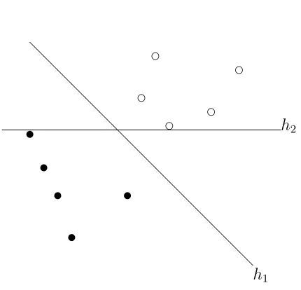
Figure 4.2: The XOR training set.
that every possible decision stump would have in-sample error 12. Thus, AdaBoost and LPBoost would terminate with one stump in the ensemble. Similarly, the Gram matrix of stump kernel is only PSD but not PD, and nonlinear hard-margin SVM with the kernel cannot find any feasible solution for this problem. In other words, those training examples cannot be perfectly separated by an ensemble over the decision stumps.
Second, the unlimited capacity has to be used with suitable regularization in order to have good generalization performance. Although SVM implicitly regularizes the admissible learning model with the large-margin concept, the unlimited capacity may still drag the algorithm towards overfitting. This situation has been observed for SVM with the Gaussian kernel (Keerthi and Lin 2003). In this situation, soft-margin SVM with a suitable parameter selection usually performs better than hard-margin SVM, because trading accuracy with larger margin further regularizes the admissible learning model.
4.1.3
Stump Kernel and Radial Basis Function
Next, we show another property of the stump kernel, which facilitates its practi-cal usage. In particular, we could drop the constant ∆S for the stump kernel KS
Theorem 10 Solving (P4) with the simplified stump kernel K˜S(x, x0) = − kx−x0k1
is the same as solving (P4) with KS(x, x0). That is, they could obtain equivalent decision functions (2.6).
Proof. Berg et al. (1984) prove that the Gram matrix of ˜KS(x, x0) = −|x−x0| is
CPSD for one-dimensional vectors x, x0. The Gram matrix of simplified stump kernel
in RD is the sum of the Gram matrix of several one-dimensional kernels, and hence
would also be CPSD. In addition, for (P4), a CPSD kernel ˜K(x, x0) works exactly the
same as any PSD kernel of the form ˜K(x, x0) + ∆ , where ∆ is a constant, because of
the linear constraint PN
i=1yiλi = 0 (Sch¨olkopf and Smola 2002; Lin and Lin 2003).
We have shown the value of ∆ = ∆S in Definition 4. Hence, the equivalence between ˜
KS and KS for (P4) can be easily established.
Let us take a closer look at this result. ˜KS(x, x0) = − kx−x0k
1 is a radial basis
function(RBF), just like the well-known Gaussian kernel. RBF is an important tool for classification, regression, interpolation, and many other learning tasks (Haykin 1999). Compared to the Gaussian kernel, the stump kernel computes the distance by one-norm, and did not use nonlinear transform of the distance. Nevertheless, the class of SVM classifiers with the stump kernel still has an infinite V-C dimension. We shall further compare them to some other types of RBF kernels in the end of this chapter.
4.1.4
Averaging Ambiguous Stumps
Theorem 11 Define (˜x)d,a as the a-th smallest value in {(xi)d}Ni=1, where xi are
the input vectors in the training set, and Ad as the number of different (˜x)d,a. Let
(˜x)d,0 =Ld, (˜x)d,(Ad+1) =Rd, and
ˆ
sq,d,a(x) =
q for (x)d ≥(˜x)d,t+1
−q for (x)d ≤(˜x)d,t
q· 2(x)d−(˜x)d,a−(˜x)d,a+1
(˜x)d,a+1−(˜x)d,a otherwise. Then,
KS(x, x0) = X
q∈{−1,+1}
D
X
d=1
Ad
X
a=0
(r(q, d, a))2sˆq,d,a(x)ˆsq,d,a(x0),
where r(q, d, a) = 12p
(˜x)d,a+1−(˜x)d,a.
We can prove Theorem 11 by carefully writing down the equations. Note that the function ˆsq,d,t(·) is not exactly a decision stump, but a smoother variant. Each ˆsq,d,t(·)
represents the group of ambiguous decision stumps in ((˜x)d,t,(˜x)d,t+1). When the
group is larger, ˆsq,d,t(·) is smoother because it represents the average prediction over
more decision stumps. Compared to LPBoost, which can use one discrete decision stump sq,d,αd(·) for αd ∈ (˜x)d,t,(˜x)d,t+1
, our framework obtains a smoother stump by averaging ambiguous decision stumps. Even though each decision stump only has an infinitesimal hypothesis weight, the representative stump ˆsq,d,t(·) could have
a concrete weight in the ensemble. This
![Figure 2.1: Illustration of the margin, where yi = 2 · I[circle is empty] − 1](https://thumb-us.123doks.com/thumbv2/123dok_us/780513.1091009/24.612.240.472.52.275/figure-illustration-margin-yi-i-circle.webp)