R E S E A R C H
Open Access
Numerical method and convergence order
for second-order impulsive differential
equations
Liangcai Mei
1*, Hongbo Sun
1and Yingzhen Lin
1*Correspondence:
1Zhuhai Campus, Beijing Institute of Technology, Zhuhai, China
Abstract
This paper is devoted to the numerical scheme for the impulsive differential equations. The main idea of this method is, for the first time, to establish a broken reproducing kernel space that can be used in pulse models. Then the uniform convergence of the numerical solution is proved, and the time consuming Schmidt orthogonalization process is avoided. The proposed method is proved to be stable and have the second-order convergence. The algorithm is proved to be feasible and effective through some numerical examples.
Keywords: Impulsive differential equations; Broken reproducing kernel space; Convergence order; Numerical algorithm
1 Introduction
Pulse boundary value problems occur in many applications: population dynamics [1],
physics, chemistry [2], irregular geometries and interface problems [3–5], signal
process-ing [6,7]. The research on the impulsive differential equations with all kinds of
bound-ary value is much more active in recent years. However, only in the last few decades has the attention been paid to the theory and numerical analysis of IDEs. All kinds of methods have been widely used to study the existence of solutions for impulsive
prob-lems [8–12]. Many researchers have extensively studied the numerical methods of
im-pulsive differential equations. Berenguer [13] provide a collage-type theorem for
impul-sive differential equations with inverse boundary conditions. Epshteyn [14,15] solved the
high-order differential equations with interface conditions based on Difference Potentials
approach for the variable coefficient. Hossainzadeh [16] applied the Adomian
Decompo-sition Method(ADM) for solving first-order impulsive differential equations. Zhang [17]
researched numerical solutions to the first-order impulsive differential equations by
collo-cation methods. Zhang [18] analyzed a class of linear impulsive delay differential equation
by asymptotic stability. Impulsive differential equation is a mathematical form of problems in many application fields, how to solve the impulsive differential equation accurately is very important.
In this paper, we consider the following second-order impulsive differential equations (IDEs for short):
⎧ ⎪ ⎪ ⎨ ⎪ ⎪ ⎩
u(x) +a1(x)u(x) +a0(x)u(x) =f(x), x∈[a,b]\{c}, u(a) =α1, u(b) =α2,
u(c) =α3, u(c) =α4,
(1)
whereu(c) =u(c+) –u(c–),α
3andα4are not at the same time as 0.ai(x) andf(x) are
known function,αj∈R,j= 1, 2, 3, 4. In this paper, only one pulse point is considered, by
that analogy, the algorithm can also be applied to multiple pulse points.
As known to all, the reproducing kernel method is a powerful tool to solve differential
equations [19–23]. However, the reproducing kernel space is smooth, in order to solve the
impulsive differential equation, for the first time, we propose a broken reproducing kernel space.
The aim of this paper is to derive the numerical solutions of Eq. (1) in Sect.1. In Sect.2, we introduce the reproducing kernel space for solving problems. Some primary results
are analyzed in Sect.3. The numerical algorithm and convergence order of approximate
solution is presented in Sect.4. In Sect.5, the presented algorithms are applied to some
numerical experiments. Then we end with some conclusions in Sect.6.
2 The reproducing kernel method
The application of reproducing kernel method in the boundary value problems has been developed by many researchers, because this method is easy to obtain the exact solution
with the series form and get approximate solution with higher precision [19,20]. However,
this method required the exact solution to be smooth, this leads to the fact that IDEs cannot be solved directly in the reproducing kernel space.
In this paper, the traditional reproducing kernel space is dealt with delicately, the space has been broken into two spaces that each one is smooth reproducing kernel space, so we
can use this space to solve IDEs. We assume that Eq. (1) have a unique solution.
2.1 The traditional reproducing kernel space
• The reproducing kernel spaceW3
2[a,c]is defined as follows:
W3
2[a,c] ={u(x)|uis an absolutely continuous real value funcion,u∈
L2[a,c]}[20] (W3
a for short).
The inner product and norm are defined as follows:
u(t),v(t)=
2
k=0
u(k)(a)v(k)(a) +
c
a
uvdt, u,v∈W23[a,c],
u=u,uw3 2.
• The reproducing kernel spaceW1
2[a,c]is defined as follows:
W1
2[a,c] ={u(x)|uis an absolutely continuous real value funcion,u∈L2[a,c]}
The inner product and norm are defined as follows:
u(t),v(t)=u(0)v(0) +
c
a
uvdt, u,v∈W21[a,c],
u=u,uw1 2.
The reproducing kernel spaces areW3
a andWa1with reproducing kernelR0t(x) andrt0(x),
respectively.
In the same way, the reproducing kernel spaces areW23[c,b] (Wb3for short) andW21[c,b] (W1
b for short) with reproducing kernelR1t(x) andr1t(x), respectively.
2.2 The reproducing kernel space with piecewise smooth
In this paper, consider that the exact solution of Eq. (1) is not a smooth function, so, we
connected two reproducing kernel spaces on both sides of the impulsive point, we call it the broken reproducing kernel space.
Definition 2.1 The linear spaceW2,3cis defined as
W2,3c[a,b] =u(x)|ifx<cthenu(x)∈Wa3, ifx≥cthenu(x)∈Wb3.
Everyu(x)∈W3
2,c[a,b] has the following form:
u(x) =
⎧ ⎨ ⎩
u0(x), x<c,
u1(x), x≥c,
whereu0(x)∈Wa3,u1(x)∈Wb3.
Theorem 2.1 Assuming that the inner product and norm in W3
2,c[a,b]are given by
u,vW3
2,c=u0,v0Wa3+u1,v1Wb3, u,v∈W 3
2,c[a,b], (2)
uW3 2,c=
u,uW3
2,c, u∈W 3 2,c[a,b]
then the space W3
2,c[a,b]is an inner space.
Proof For anyu,v,w∈W2,3c[a,b],
u+v,wW3
2,c=u0+v0,w0Wa3+u1+v1,w1Wb3
=u0,w0Wa3+v0,w0Wa3+u1,w1Wb3+v1,w1Wb3
=u,wW3
2,c+v,wW2,3c.
We can prove that Eq. (2) satisfies the other requirements of the inner product space.
Proof Suppose that{un(x)}∞n=1is a Cauchy sequence inW2,3c[a,b], however,
Theorem 2.3 The space W2,3c[a,b]is a reproducing kernel space with the reproducing ker-nel function
Similarly, the reproducing kernel spaceW1
2,c[a,b] is defined as
W2,1c[a,b] =u(x)|ifx<cthenu(x)∈Wa1, ifx≥cthenu(x)∈Wb1 (4)
and it has the reproducing kernel function
In order to solve Eq. (1), we introduce a linear operatorL:W2,3c[a,b]→W1 2,c[a,b],
Lu=u(x) +a1(x)u(x) +a0(x)u(x), u∈W2,3c[a,b].
By Ref. [20], it is easy to prove thatLis a bounded operator.
Then Eq. (1) can be transformed into the following form:
⎧
In this section, the approximate solution of Eq. (6) is presented in the reproducing kernel
spaceW3
2,c[a,b]. And the convergence of the approximate solution is proved, discuss the
approximate solution of the situation and the range of error.
then
The unique solution to the above equations exists (see [20]), then
and
Pnu,∅1W2,3c=u,Pn∅1W2,3c=u,∅1W2,3c=u,RaW2,3c=u(a) =α1.
Similarly, we have
Pnu,∅2=α2, Pnu,∅3=α3, Pnu,∅4=α4.
So,Pnuis the solution of Eq. (7).
In fact,un(x) is an approximate solution of the exact solution.
Theorem 3.4 If u∈W3
2,c[a,b]is the solution of Eq. (6),put un=Pnu∈Snthen unconverges
uniformly to u.
Proof
u(t) –un(t)=
u–un,
∂Rt
∂t
≤∂Rt
∂t
W3 2,c
u–unW3 2,c
≤Mu–unW3
2,c→0.
Similarly, we can prove that ift∈[a,c] and [c,b], respectively, thenu(ni)converges
uni-formly tou(i),i= 1, 2.
In order to analyze the convergence order of the algorithm proposed in this section, we derive the following lemma.
Lemma 3.1 ([20]) If un=Pnu is the approximate solution ofLu=f(x),L:W23[a,b]→ W1
2[a,b]is a linear operator,then
u(i)–un(i)≤Mih2, i= 0, 1.
Theorem 3.5 The approximate solution un=Pnu of Eq. (6)converges to its exact solution
u with not less than second-order convergence.
Proof By Definition2.1, we get
u(x) =
⎧ ⎨ ⎩
u0(x), x<c,
u1(x), x≥c.
In addition,un=Pnuis converges uniformly touby Theorem3.4. So, there areu0,nand
u1,nsatisfying the following expressions:
u(x) –un(x)
2
W3 2,c=
u0(x) –u0,n(x)
2
W3
a+u1(x) –u1,n(x) 2
W3
b →0.
So,u0(x) –u0,n(x)2W3
a→0,u1(x) –u1,n(x) 2
Note thatu0,n(x) is the approximate solution ofLu=f(x) in reproducing kernel space
Wa3, take advantage of Lemma3.1, we have
u0(x) –u0,n(x)≤M0h2.
Similarly, we have|u1(x) –u1,n(x)| ≤M1h2.
For anyx∈[a,b]
u(x) –un(x)≤maxu0(x) –u0,n(x),u1(x) –u1,n(x)≤max
M0h2,M1h2
=M2h2.
Herehis step-size on the interval [a,b],M0,M1,M2are constants. Therefore,un
con-verges tounot less than the second-order convergence.
Furthermore, the following rate of convergence formulas can be obtained:
C.R=log2 |u(x) –un(x)|
|u(x) –u2n(x)|
.
By the results of this section, the exact solution of Eq. (6) can be expressed as
u(x) =
∞
i=1
λiψi(x) +k1∅1(x) +k2∅2(x) +k3∅3(x) +k4∅4(x). (8)
4 Numerical algorithm
In this section, the numerical algorithm for the approximate solutionunis given. Now, the
solutionunof Eq. (7) is the approximate solution of Eq. (1). Asun∈Sn, so
un(x) = n
i=1
λiψi(x) +k1∅1(x) +k2∅2(x) +k3∅3(x) +k4∅4(x). (9)
To obtain the approximate solutionun, we only need to obtain the coefficients of each
ψi(x),i= 1, 2, . . . ,nand∅j(x),j= 1, 2, 3, 4. Useψi(x) and∅j(x) to do the inner products with
both sides of Eq. (9), we have
⎧ ⎨ ⎩
n
j=1λjψj,ψi+
4
j=1kjψi,∅j=f(xi), i= 1, 2, . . . ,n,
n
j=1λjψj,∅i+
4
j=1kj∅i,∅j=αi, i= 1, 2, 3, 4.
(10)
This is the system of linear equations ofλi,kj,i= 1, 2, . . . ,n,j= 1, 2, 3, 4.
Let
Gn+4= ⎡ ⎢ ⎣
ψi,ψk · · · ψi,∅j · · · · ψk,∅j · · · ∅j,∅m
⎤ ⎥ ⎦
i,k=1,2,...,n;j,m=1,2,3,4
,
F=f(x1),f(x2), . . . ,f(xn),α1,α2,α3,α4 T
Consider that{ψi(x)}ni=1∪ {∅j(x)}4j=1is linearly independent inW2,3c[a,b]; therefore,G–1
exists. Then we have
(λ1, . . . ,λn,k1,k2,k3,k4)T=G–1·F.
5 Numerical examples
In this section, the method proposed in this paper is applied to some impulsive differential
equations to evaluate the approximate solution. In Examples1–3, the reproducing space
isW3
2,c[0, 1]. We compare the numerical results with the other methods discussed in [13,
14]. Finally, the results show that our algorithm is practical and remarkably effective.
Example1 (Ref. [13]) Consider the linear impulsive differential equation
⎧ ⎪ ⎪ ⎨ ⎪ ⎪ ⎩
–u(x) +u(x) = 0, a.e. x∈(0, 1),
u(0) = 0, u(1) = –1,
u(1/4) = –2, u(1/4) = 0.
The exact solution
u(x) =
⎧ ⎨ ⎩
e14 –x(–1–e34+e32)(e2x–1)
e2–1 , x∈[0,14],
e– 14 –x(e2x–e2x+ 12–e2x+ 54+e54–e2+e52)
e2–1 , x∈(14, 1].
The numerical results are given in Table 1, where the rate of convergence C.R=
log2||uu((xx)–)–uun(x)|
2n(x)|, from the comparison with method in [13], we confirm that our algorithm
satisfies Theorem3.5. It shown that the present method can produce a more accurate
ap-proximate solution.
Example2 (Ref. [13]) Consider the following equation with two pulse points:
⎧ ⎪ ⎪ ⎪ ⎪ ⎪ ⎨ ⎪ ⎪ ⎪ ⎪ ⎪ ⎩
–u(x) = 0, a.e. x∈(0, 1),
u(0) = 0, u(1) = 0,
u(1
3) = –1, u(
1 3) = 0,
u(45) = 1, u(45) = 0.
Table 1 Comparison of absolute errors in Example1
n |u(x) –un(x)|[13] Presented method
max|u–un| C.R max|u–un| C.R max|u–un|
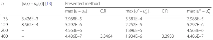
33 3.426E–3 7.988E–5 3.381E–4 7.988E–5
129 8.562E–4 5.297E–6 2.252E–5 5.297E–6
200 – 4.563E–6 1.896E–5 4.563E–6
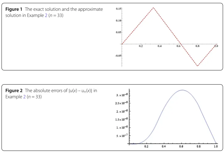
Figure 1The exact solution and the approximate solution in Example2(n= 33)
Figure 2The absolute errors of|u(x) –un(x)|in Example2(n= 33)
Table 2 Comparison of absolute errors in Example2
n max|u(x) –un(x)|[13] Presented method
max|u(x) –un(x)| C.R max|u(x) –un(x)| C.R
33 4.627F–2 3.299F–6 1.197F–5
129 1.578F–5 2.028F–7 8.090F–7
400 – 2.048F–8 8.238F–8
800 – 5.022F–9 2.0271 2.028F–8 2.0222
The exact solution
u(x) =
⎧ ⎪ ⎪ ⎨ ⎪ ⎪ ⎩ 7x
15, x∈[0, 1 3], 1
3– 8x
15, x∈( 1 3,
4 5],
–157 –715x, x∈(45, 1].
In Fig.1, the red dotted line is the numerical solution and the black line is the exact
solution. Figure2shows the absolute error|u(x) –un(x)|whenn= 33. Table2shows
com-parison of the absolute errors between our method and other methods. All graphs and tables show that our method is effective as we expect. It is worth noting that the
approx-imate solutions of Example1and Example2are only proved norm of convergence to the
exact solutions (see [13]). But, the approximate solutions of this paper are proved
uni-formly converges tou(x).
Example 3 (Ref. [14]) Consider the following impulsive equation with variable coeffi-cients:
(βux)x= 56x6, x∈[0, 1]{0.5}, whereβ=
⎧ ⎨ ⎩
1, x∈[0, 0.5],
Table 3 Comparison of absolute errors in Example3
n |u(x) –un(x)|[14] Presented method
max|w(x) –un(x)| C.R max|u(x) –un(x)| C.R
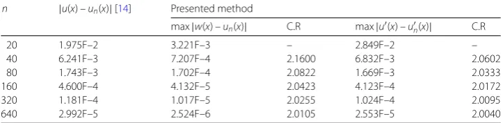
20 1.975F–2 3.221F–3 – 2.849F–2 –
40 6.241F–3 7.207F–4 2.1600 6.832F–3 2.0602
80 1.743F–3 1.702F–4 2.0822 1.669F–3 2.0333
160 4.600F–4 4.132F–5 2.0423 4.123F–4 2.0172
320 1.181F–4 1.017F–5 2.0255 1.024F–4 2.0095
640 2.992F–5 2.524F–6 2.0105 2.553F–5 2.0040
subject to the boundary and interface conditions:
⎧
Table3lists the absolute error and the rate of convergence C.R to Example3, from the
illustrative tables, we conclude that when truncation limitnis increased we can obtain a
good accuracy. It shows that the proposed approach is very stable and effective.
The proposed method not only can solve Eq. (1) of impulsive differential equation, but
also can solve high-order impulsive differential equations and complex boundary value problems of pulse. The theory and algorithm is similar, we use the following example to prove the effectiveness of the algorithm.
Example4 Consider the third-order linear impulsive differential equation
Table 4 Comparison of absolute errors in Example4
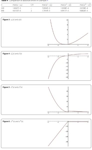
n max|u–un| C.R max|u–un| max|u–un| max|u–un|
320 1.8367F–5 – 7.0934F–5 1.9598F–4 3.9198F–4
640 4.6155F–6 2 1.7919F–5 4.9411F–5 9.8826F–5
Figure 3 un(x) andu(x)
Figure 4 un(x) andu(x)
Figure 5 u(x) andu(x)
Figure 6 u(x) andu(x)
In the Example4, the reproducing space isW4
2,c[–2, 2]. Table4shows the absolute errors
and convergence order of our method in different cases. In Figs.3–6, the red dotted line
6 Conclusion
In this paper, it is the first time to apply the reproducing kernel method to solve the impul-sive differential equations. A broken reproducing kernel space is cleverly built, the repro-ducing space are reasonably simple because the author did not consider the complicated boundary conditions, and avoid the time consuming Schmidt orthogonalization process, and the approximate solution we get is no less than the second-order convergence. In
Sect.5, Numerical examples, we do four experiments with the new algorithm, and make a
comparison with other algorithms. In fact, this technique can be extended to other class of impulsive boundary value problems. Although we just considered one pulse point in our presentation, by that analogy, the algorithm can also be applied to multiple pulse points. From the illustrative tables and figures, we find that the algorithm is remarkably accurate and effective as expected.
Acknowledgements
The authors are grateful for the comments of the referee, which have improved the exposition of this paper. Funding
This work has been supported by 2018KQNCX338, a Young Innovative Talents Program in Universities and Colleges of Guangdong Province, and XT-2018-03, a Scientific Research-Innovation Team Project at Zhuhai Campus, Beijing Institute of Technology.
Availability of data and materials
All data generated or analyzed during this study are included in this published article. Ethics approval and consent to participate
I declare that the papers submitted are the results of research by all of our authors. Competing interests
The authors declare that no competing interests exist. Consent for publication
The author agrees to publish it in this journal. Authors’ contributions
LM conceived of the study, designed the study and collected the literature. HS proved the convergence of the algorithm. YL reviewed the full text. All authors were involved in writing the manuscript. All authors read and approved the final manuscript.
Publisher’s Note
Springer Nature remains neutral with regard to jurisdictional claims in published maps and institutional affiliations.
Received: 24 August 2018 Accepted: 4 June 2019
References
1. Bainov, D.D., Dishliev, A.B.: Population dynamics control in regard to minimizing the time necessary for the regeneration of a biomass taken away from the population. Appl. Math. Comput.39(1), 37–48 (1990)
2. Bainov, D.D., Simenov, P.S.: Systems with Impulse Effect Stability Theory and Applications. Ellis Horwood, Chichester (1989)
3. LeVeque, R.J., Li, Z.: Immersed interface methods for Stokes flow with elastic boundaries or surface tension. SIAM J. Sci. Comput.18(3), 709–735 (2012)
4. Huang, Y., Forsyth, P.A., Labahn, G.: Inexact arithmetic considerations for direct control and penalty methods: American options under jump diffusion. Appl. Numer. Math.72(2), 33–51 (2013)
5. Liu, X.D., Sideris, T.C.: Convergence of the ghost fluid method for elliptic equations with interfaces. Math. Comput.
72(244), 1731–1746 (2013)
6. Cao, S., Xiao, Y., Zhu, H.: Linearized alternating directions method forl(1)-norm inequality constrainedl(1)-norm minimization. Appl. Numer. Math.85, 142–153 (2014)
7. Candes, E.J., Romberg, J., Tao, T.: Robust uncertainty principles: exact signal reconstruction from highly incomplete frequency information. IEEE Trans. Inf. Theory52(2), 489–509 (2006)
8. Wang, Q., Wang, M.: Existence of solution for impulsive differential equations with indefinite linear part. Appl. Math. Lett.51, 41–47 (2016)
10. Jankowski, T.: Positive solutions to second order four-point boundary value problems for impulsive differential equations. Appl. Math. Comput.202(2), 550–561 (2008)
11. Bogun, I.: Existence of weak solutions for impulsive-Laplacian problem with superlinear impulses. Nonlinear Anal., Real World Appl.13(6), 2701–2707 (2012)
12. Wang, J.R., Zhou, Y., Lin, Z.: On a new class of impulsive fractional differential equations. Appl. Math. Comput.242, 649–657 (2014)
13. Berenguer, M.I., Kunze, H., Torre, D.L., Galan, M.R.: Galerkin method for constrained variational equations and a collage-based approach to related inverse problems. J. Comput. Appl. Math.292, 67–75 (2016)
14. Epshteyn, Y., Phippen, S.: High-order difference potentials methods for 1D elliptic type models. Appl. Numer. Math.
93, 69–86 (2015)
15. Epshteyn, Y.: Algorithms composition approach based on difference potentials method for parabolic problems communications. Commun. Math. Sci.12(4), 723–755 (2014)
16. Hossainzadeh, H., Afrouzi, G., Yazdani, A.: Application of Adomian decomposition method for solving impulsive differential equations. J. Math. Comput. Sci.2(4), 672–681 (2011)
17. Zhang, Z., Liang, H.: Collocation methods for impulsive differential equations. Appl. Math. Comput.228(228), 336–348 (2014)
18. Zhang, G.L., Song, M.H., Liu, M.Z.: Asymptotic stability of a class of impulsive delay differential equations. J. Appl. Math.
10, 487–505 (2012)
19. Cui, M., Lin, Y.: Nonlinear Numerical Analysis in the Reproducing Kernel Space. Nova Science Publishers, New York (2009)
20. Wu, B., Lin, Y.: Application of the Reproducing Kernel Space. Science Press (2012)
21. Zhao, Z., Lin, Y., Niu, J.: Convergence order of the reproducing kernel method for solving boundary value problems. Math. Model. Anal.21(4), 466–477 (2016)
22. Mei, L., Jia, Y., Lin, Y.: Simplified reproducing kernel method for impulsive delay differential equations. Appl. Math. Lett.
83, 123–129 (2018)