R E S E A R C H
Open Access
Sustained oscillation induced by time
delay in a commodity market model
Kejun Zhuang
1,2*and Gao Jia
3*Correspondence: [email protected]
1Business School, University of Shanghai for Science and Technology, Shanghai, 200093, China
2School of Statistics and Applied Mathematics, Anhui University of Finance and Economics, Bengbu, 233030, China
Full list of author information is available at the end of the article
Abstract
In this paper, the existence of local and global Hopf bifurcation for a delay commodity market model is studied in detail. As time delay increases, the commodity price will fluctuate periodically. Furthermore, such fluctuations will occur even if the time delay is sufficiently large.
MSC: 91B55; 34K18
Keywords: commodity market model; stability; global Hopf bifurcation
1 Introduction
In most economic and financial processes, mathematical modeling leads to nonlinear de-layed dynamical systems, and the interplay of dede-layed and nonlinear effects is important for many reasons. Capturing the price behavior of commodity and forecasting future de-velopments are essential in commodity management and international policy. Given this, fluctuations in commodity price have long been, and will continue to be, one of the dom-inant topics in mathematical economics due to its universal existence and importance. Based on some mathematical assumptions, various price adjustment models have been de-veloped to analyze the problems in economics, see [–] and the references cited therein. One of the representative models was introduced by Mackey [, ], who considered a price adjustment model for a single commodity market with state dependent production and storage delays in the following form:
P(t)
P(t) =D
P(t)–SPs(t). ()
HereP(t) is the market price of a particular commodity at timet, andDandSrefer to demand and supply functions, respectively. It is assumed that the consumers base their buying decisions on current market prices. For most commodities, there is a finite timeτ
that elapses before a change in production occurs. Assuming that only the market price at timet–τhas an effect on the current supply pricePs(t), we getPs(t) =P(t–τ) (see [] for more details). Farahani and Grove [] considered the following special case:
P(t)
P(t) =
a b+Pn(t)–
cPm(t–τ)
d+Pm(t–τ), ()
wherea,b,c,d,m,τ> , andn≥. For system (), global convergence of the positive equi-librium was investigated in [, ], global attractivity of solutions was discussed in []. In addition, the existence of almost periodic solutions for an impulsive delay model was established in [, ].
However, the dynamic behaviors of system () still need further investigation. In this paper, we are trying to improve the understanding of the complex dynamics induced by time delay. Motivated by the conjecture on global bifurcation results in [], we shall focus on the global continuation of a local Hopf bifurcation. In the following sections, the sta-bility of a unique positive equilibrium and a local Hopf bifurcation analysis for system () are presented. After that, the global existence of bifurcating periodic solutions is explored with the assistance of global Hopf bifurcation theory developed by Wu [], and related applications can be found in [–]. Finally, some numerical simulations are performed to illustrate the theoretical results.
2 Local Hopf bifurcation analysis
In light of the monotonicity of demand and supply functions, system () has a unique positive equilibriumP∗ such thata/(b+Pn∗) =cPm∗/(d+Pm∗). Based on Taylor’s formula,
the linearized system of () atP∗is as follows:
dP
dt = –αP(t) –βP(t–τ), ()
whereα=anP∗n/(b+P∗n)> andβ=cdmPm∗/(d+Pm∗)> . When we define thatP(t) =eλt and substitute it into (), we can get the following first order transcendental characteristic equation:
λ+α+βe–λτ= . ()
It is evident that the characteristic root isλ= –(α+β) < whenτ= . On the other hand, equation () has infinitely many roots asτ > , and these roots vary withτ. According to Corollary . in [], the sum of characteristic roots in the open right half-plane can change only if a root appears on or crosses the imaginary axis. In order to establish the number of roots with positive real parts, we assume thatλ=iω(ω> ) is a root of (). Then
iω+α+β(cosωτ–isinωτ) = .
By separating the real and imaginary parts, we get the following:
α+βcosωτ= ,
ω–βsinωτ= .
Adding the squares of both equations together gives the following:
ω=β–α.
Clearly, equation () has a pair of purely imaginary roots±iω whenβ>α andτ =τk (k= , , , . . .), where
ω=
β–α, τ k=
ω
arccos–α
β + kπ
Then we verify the transversality condition. Letλk=ηk(τ) +iωk(τ) denote a root of ()
Due to the above inequality, we can deduce that the number of characteristic roots with positive real parts will increase by two when time delayτ passes the critical valuesτkeach time.
Through the above analysis, we can determine the distribution of roots of () as follows.
Lemma For equation(),the following claims are true:
(i) Ifβ≤α,then all roots of()have negative real parts for anyτ ≥.
(ii) Ifβ>α,then()has a pair of imaginary roots±iωwhenτ=τk(k= , , , . . .).
(iii) Ifβ>α,then all roots of()have negative real parts only whenτ∈[,τ).Equation
()has(k+ )roots with positive real parts whenτ ∈(τk,τk+].
According to the results regarding the stability of equilibrium in [], we have the follow-ing theorem about the stability of positive equilibrium and the existence of a local Hopf bifurcation.
Theorem For system(),we have:
(i) ifβ≤α,then the positive equilibriumP∗is asymptotically stable;
(ii) ifβ>α,then the positive equilibriumP∗is stable whenτ<τand unstable when
τ>τ.Moreover,a Hopf bifurcation occurs at the critical valueτk,and periodic
solutions will bifurcate fromP∗.
For convenience, we rewrite some notations as follows:
Following the algorithms in [, ], we can obtain the crucial coefficients which will be used in determining the bifurcation properties:
g=Dτ
Consequently, we can calculate the following quantities:
c() =
(β> );T determines the period of the bifurcating periodic solutions: the period in-creases (dein-creases) ifT> (T< ).
It is not difficult to find that the derivatives of demand and supply functions at the pos-itive equilibriumP∗have significant effects on the properties of a local Hopf bifurcation. 3 Global bifurcation analysis
It is known that periodic solutions through Hopf bifurcation are generally local and only exist in a small neighborhood of the critical value. Hence it is interesting and significant to verify the global existence of bifurcating periodic solutions. In this section, we study the global continuation of periodic solutions bifurcating from the positive equilibriumP∗of
system ().
Following the work of [], we need to show the uniform boundedness of the periodic solutions of () and the nonexistence ofτ-periodic solutions.
Lemma If a>bc,and m and n are even integers,then all periodic solutions of()are uniformly bounded.
Proof LetP(t) be a nonconstant periodic solution of () and define that
A=P(t) =max
From the second equation and the even quality ofmandn, we have
Lemma If m and n are even,then system()has noτ-periodic solution.
Proof Assume that system () has aτ-periodic solution, then the following ordinary dif-ferential equation
dP
dt =P(t)
a b+Pn(t)–
cPm(t)
d+Pm(t) ()
has a nonconstant periodic solution.
Becausemandnare even integers, system () has three steady statesP(t) = ,P(t) =P∗
andP(t) = –P∗. In system (),P˙(t) < holds whenP(t) >P∗or –P∗<P(t) < , andP˙(t) >
holds when <P(t) <P∗ orP(t) < –P∗. Therefore, the ordinary differential equation () does not have a nonconstant periodic solution. This implies that system () has noτ
-periodic solution. The proof is complete.
We then have the following theorem about the global existence of a Hopf bifurcation.
Theorem Suppose that a>bc,β>α,and m and n are even.Then,for eachτ>τk,k=
, , , . . . ,system()still has positive periodic solutions.
Proof For the convenience of using the results from [], we rewrite () as the following functional differential equation:
˙
x(t) =F(xt,τ,p), ()
which satisfies the conditions (A)-(A) in []. Following the notations there, we have the following:
Δ(x,τ,p)(λ) =λ+α+βe
–λτ
.
Herexis the equilibrium of (). It is easy to verify that (x,τk, π/ω) are isolated centers. Then there existε> ,δ> and a smooth functionλ: (τj–δ,τj+δ)→Csuch that
Δλ(τ)= , λ(τ) –iω<ε
for anyτ∈[τk–δ,τk+δ], and
λ(τk) =iω,
dRe(λ(τ)) dτ > .
Define that p= π/ωandΩε,p ={(,p) : <u<ε,|p–p|<ε}. If|τ–τk| ≤δ and
(u,p)∈∂Ωε, thenΔ(x,τ,p)(u+ πi/p) = if and only ifτ=τk,u= ,p=pk. Thus,
assump-tion (A) in [] holds.
Next introducing a function defined by
yields the crossing number
γ(x,τj, π/ω) =degB
H–(x,τk, π/ω),Ωε,p
–degBH+(x,τk, π/ω),Ωε,p
= – .
Thus the connected componentC(x,τk, π/ω) through (x,τk, π/ω) is nonempty, and
(x,τ,p)∈C(x,τk,π/ω)
γ(x,τ,p) < ,
which implies thatC(x,τk, π/ω) is unbounded. From Lemmas and , we know that the projection ofC(x,τk, π/ω) onto thex-space is bounded and that onto theτ-space is away from zero.
For a contradiction, we suppose that the projection ofC(x,τk, π/ω) ontoτ-space is bounded. This means that the projection ofC(x,τk, π/ω) ontoτ-space is included in an interval (,τ∗).
From the definition ofτkin Section , we can get that
π
<ωτ<π, and kπ<ωτk< (k+ )π< (k+ )π, k≥.
Hence,
τ< π ω
< τ, and
τk
k+ < π ω
<τk
k, k≥,
and we have τ<p< τ if (x(t),τ,p)∈C(x,τ, π/ω), τ/ <p<τ if (x(t),τ,p)∈
C(x,τ, π/ω), andτ/ <p<τ/ if (x(t),τ,p)∈C(x,τ, π/ω), and so on. This im-plies that the projection ofC(x,τk, π/ω) ontop-space is bounded. As a result, we can determine that the connected componentC(x,τk, π/ω) is bounded. This leads to a
con-tradiction and the proof is complete.
4 Numerical examples
To support the theoretical analysis, we consider the following system:
P(t) =P(t)
. . +P(t)–
.P(t–τ)
. +P(t–τ) . ()
Through a direct computation, we can determine P∗ = ., α = ., β =
.,ω= . andτk=.+.kπ,τ= .,τ= .,τ= .,τ= ., . . . .
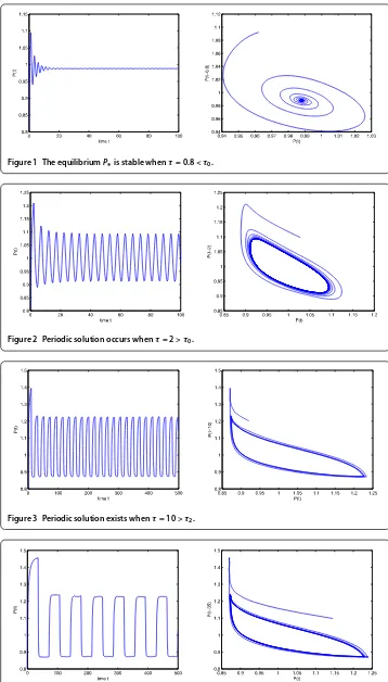
From Figures and , we can find that a Hopf bifurcation occurs when time delay τ
Figure 1 The equilibriumP∗is stable whenτ= 0.8 <τ0.
Figure 2 Periodic solution occurs whenτ= 2 >τ0.
Figure 3 Periodic solution exists whenτ= 10 >τ2.
we can see that time delay has a major impact on the dynamics of commodity market model (). We can also find that the amplitude and period of the periodic solution will increase gradually as time delay increases.
Thus, our theoretical results and numerical simulations show that the time delay has a substantial effect on the periodic dynamic behaviors in commodity market model ().
5 Conclusions
This paper presents the results of an investigation into the existence of local and global Hopf bifurcations for a price adjusting model with time delay. It can be concluded that time delay may destabilize the equilibrium of that model and induce periodic oscillations. Moreover, the periodic oscillations will persist even when the delay is sufficiently large, which indicates the global existence of a Hopf bifurcation in the model. Thus, the results obtained here can supplement the previous literature and help people to understand price fluctuation mechanisms.
However, from another perspective, we sometimes need to control commodity price fluctuations, and one effective method is to shorten the time between the initiation of changes in production and the final alteration of supply. More specifically, the finite de-lay τ is the time between production and price changes. As we know, large delay may induce complex dynamical behaviors, such as drastic periodic fluctuations. Therefore, timely price adjustments are necessary, which can effectively reduce the time delay. Math-ematically, we should stabilize the positive equilibrium and control the Hopf bifurcation, and we will consider this in our work in the near future.
Competing interests
The authors declare that they have no competing interests.
Authors’ contributions
All authors have equally contributed to this paper. They have read and approved the final version of the manuscript.
Author details
1Business School, University of Shanghai for Science and Technology, Shanghai, 200093, China.2School of Statistics and Applied Mathematics, Anhui University of Finance and Economics, Bengbu, 233030, China.3College of Science, University of Shanghai for Science and Technology, Shanghai, 200093, China.
Acknowledgements
This work is supported by the Key Project for Excellent Young Talents Fund Program of Higher Education Institutions of Anhui Province (gxyqZD2016100) and the Anhui Provincial Natural Science Foundation (1508085MA09 and
1508085QA13).
Received: 7 September 2016 Accepted: 3 February 2017
References
1. Diamond, PA: A model of price adjustment. J. Econ. Theory3, 156-168 (1971)
2. Davis, EG: A dynamic model of the regulated firm with a price adjustment mechanism. Bell J. Econ. Manag. Sci.4, 270-282 (1973)
3. Muresan, AS, Iancu, C: A new model of price fluctuation for a single commodity market. Semin. Fixed Point Theory Cluj-Napoca3, 277-280 (2002)
4. Westerhoff, F, Reitz, S: Commodity price dynamics and the nonlinear market impact of technical traders empirical evidence for the US corn market. Physica A349, 641-648 (2005)
5. Mackey, MC: Commodity price fluctuations: price dependent delays and nonlinearities as explanatory factors. J. Econ. Theory48, 497-509 (1989)
6. Bélair, J, Mackey, MC: Consumer memory and price fluctuations in commodity markets an integrodifferential model. J. Dyn. Differ. Equ.1, 299-325 (1989)
7. Farahani, AM, Grove, EA: A simple model for price fluctuations in a single commodity market. In: Oscillation and Dynamics in Delay Equations, San Francisco, CA, 1991. Contemp. Math., vol. 129, pp. 97-103. Am. Math. Soc., Providence (1992)
8. Liz, E, Röst, G: Global dynamics in a commodity market model. J. Math. Anal. Appl.398, 707-714 (2013)
10. Qian, C: Global attractivity in a delay differential equation with application in a commodity model. Appl. Math. Lett. 24, 116-121 (2011)
11. Stamov, GT, Alzabut, JO, Atanasov, P, Stamov, AG: Almost periodic solutions for an impulsive delay model of price fluctuations in commodity markets. Nonlinear Anal., Real World Appl.12, 3170-3176 (2011)
12. Stamov, GT, Stamov, AG: On almost periodic processes in uncertain impulsive delay models of price fluctuations in commodity markets. Appl. Math. Comput.219, 5376-5383 (2013)
13. Wu, J: Symmetric functional differential equations and neural networks with memory. Trans. Am. Math. Soc.350, 4799-4838 (1998)
14. Wei, J, Li, MY: Hopf bifurcation analysis in a delayed Nicholson blowflies equation. Nonlinear Anal.60, 1351-1367 (2005)
15. Riad, D, Hattaf, K, Yousfi, N: Dynamics of a delayed business cycle model with general investment function. Chaos Solitons Fractals85, 110-119 (2016)
16. Wang, Y, Jiang, W, Wang, H: Stability and global Hopf bifurcation in toxic phytoplankton-zooplankton model with delay and selective harvesting. Nonlinear Dyn.73, 881-896 (2013)
17. Sun, X, Wei, J: Global existence of periodic solutions in an infection model. Appl. Math. Lett.48, 118-123 (2015) 18. Ruan, S, Wei, J: On the zeros of transcendental functions with applications to stability of delay differential equations
with two delays. Dyn. Contin. Discrete Impuls. Syst., Ser. A Math. Anal.10, 863-874 (2003) 19. Hale, JK, Lunel, SMV: Introduction to Functional Differential Equations. Springer, New York (1993)
20. Hassard, BD, Kazarinoff, ND, Wan, YH: Theory and Applications of Hopf Bifurcation. Cambridge University Press, Cambridge (1981)