Muon g – 2 theory: The hadronic part

Muon

g

₋

2

theory:

T

he

hadronic

part

FredJegerlehner1,2,

1_{Deutsches Elektronen–Synchrotron (DESY), Platanenallee 6, D–15738 Zeuthen, Germany} 2_{Humboldt–Universität zu Berlin, Institut für Physik, Newtonstrasse 15, D–12489 Berlin, Germany}

Abstract. I present a status report of the hadronic vacuum polarization effects for the muong₋2, to be considered as an update of [1]. The update concerns recent new inclusive

Rmeasurements from KEDR in the energy range 1.84 to 3.72 GeV. For the leading order contributions I findahad(1)

µ =(688.07±4.14)[688.77±3.38]×10−10based one+e−data [incl. τdata],ahad(2)

µ =(−9.93±0.07)×10−10(NLO) andahad(3)µ =(1.22±0.01)×10−10(NNLO).

Collecting recent progress in the hadronic light-by-light scattering I adoptπ0, η, η[95±

12]+axial–vector [8_±3]+scalar [₋6_±1]+π,Kloops [−20±5]+quark loops [22_±4] +tensor [1± 0]+NLO [3± 2] which yieldsa(6)µ (lbl,had)=(103±29)×10−11.With

these updates I findaexpµ −atheµ =(31.3±7.7)×10−10a 4.1σdeviation. Recent lattice

QCD results and future prospects to improve hadronic contributions are discussed.

1 Overview: hadronic effects in

g

₋

2.

This review of the hadronic vacuum polarization (HVP) contributions to the muong₋2 is to be con-sidered as a complement to the theory reviews by Marc Knecht and Massimiliano Procura which focus on the hadronic light-by-light (HLbL) part and the reviews on hadronic cross sections by Graziano Venanzoni, Simon Eidelman and Achim Denig in these Proceedings.

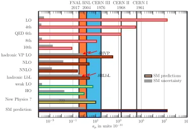
The present experimental muon g−2 result from Brookhaven (BNL) aexpµ = (11 659 209.1± 5.4±3.3[6.3])×10−10 _{[2] soon will be improved by the new muong−2 experiments at Fermilab} and J-PARC. The Fermilab experiment will be able to reduce the error by a factor 4, the J-PARC experiment will provide an important cross check with a very different technique [3]. It means that the new muong−2 experiments are expected to establish a possible new physics contribution at the level∆aµ =aexpµ −atheµ =6.7σprovided theory remains as it is today and the central value does not move significantly. If we achieve a reduction of the hadronic uncertainty by factor 2 we would arrive at∆aµ=11.6σ. That’s what we hope to achieve. Figure 1 illustrates the present status and what has been achieved so far. The present resultsaHVP LO

µ =(6888±34)×10−11amounts to+59.09±0.30 ppm, which poses the major challenge. The subleading resultsaHVP NLO

µ =(−99.3±0.7)×10−11and

aHVP NNLO

µ =(12.2±0.1)×10−11 although relevant will be known well enough. These number also compare with the well established weakaEW

µ =(154±1)×10−11at 1.3±0.0 ppm and the problematic HLbL estimated to contributeaHLbL

µ =(103±29 [105±26])×10−11, which is representing a+0.90

±0.25 ppm effect.

aµin units 10−11

10−3 ₁₀−1 ₁₀1 ₁₀3 ₁₀5 ₁₀7 ₁₀9

FNAL BNLCERN III CERN II CERN I

2017 2004 1976 1968 1961

LO 4th QED 6th 8th 10th

hadronic VP LO

NLO

NNLO

hadronic LbL weak LO HO

New Physics ?

SM prediction

???

SM predictions SM uncertainty

δHVP

δHLbL

Figure 1. Past and futureg₋2 experiments testing various contributions. As New Physics ? we display the deviation (aexp

µ −atheµ )/aexpµ . Arrows point to what is limiting theory precision presently: the Hadronic Vacuum

Polarization (HVP) and Hadronic Light-by-Light (HLbL) contributions.

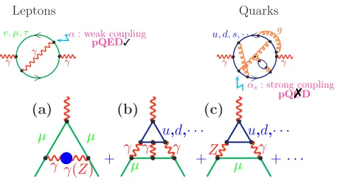
Virtual effect form low energy hadronic excitations are the standard problem in elec-troweak precision physics. At a certain level of precision predictions are hampered by non-perturbative effects, which technically are not under desirable control on the theory side. For the muon g−2 the leading hadronic effects are related to the diagrams in figure 2 and concern

(a) Hadronic vacuum polarization (HVP) of orderO(α2),O(α3),

(b) Hadronic light-by-light scattering (HLbL) of orderO(α3),

(c) Hadronic effects in 2-loop hadronic electroweak (HEW) corrections of order sub–O(αGFm2µ). Light quark loops appear as non-perturbative hadronic “blobs”. The evaluation of the corresponding non-perturbative effects relies on hadron production data in conjunction with Dispersion Relations (DR), or on low energy effective modeling by the Resonance Lagrangian Approach (RLA), specifi-cally by the Hidden Local Symmetry (HLS) model [4], or the Extended Nambu–Jona-Lasinio (ENJL) model [5], large–NcQCD inspired methods [6] and on lattice QCD. Different strategies apply for the different kinds of contributions:

(a) HVP one evaluates via a dispersion integral overe+_e− _{→hadrons data. Here 1 independent} amplitude is to be determined by one specific data set. Global fits based on the RLA (like HLS) allow to improve the data-driven evaluations [7]. Lattice QCD is the ultimate tool to get QCD predictions in future.

chi-aµin units 10−11

10−3 ₁₀−1 ₁₀1 ₁₀3 ₁₀5 ₁₀7 ₁₀9

FNAL BNLCERN III CERN II CERN I

2017 2004 1976 1968 1961

LO 4th QED 6th 8th 10th

hadronic VP LO

NLO

NNLO

hadronic LbL weak LO HO

New Physics ?

SM prediction ??? SM predictions SM uncertainty δHVP δHLbL

Figure 1. Past and futureg₋2 experiments testing various contributions. As New Physics ? we display the deviation (aexp

µ −atheµ )/aexpµ . Arrows point to what is limiting theory precision presently: the Hadronic Vacuum

Polarization (HVP) and Hadronic Light-by-Light (HLbL) contributions.

Virtual effect form low energy hadronic excitations are the standard problem in elec-troweak precision physics. At a certain level of precision predictions are hampered by non-perturbative effects, which technically are not under desirable control on the theory side. For the muon g −2 the leading hadronic effects are related to the diagrams in figure 2 and concern

(a) Hadronic vacuum polarization (HVP) of orderO(α2),O(α3),

(b) Hadronic light-by-light scattering (HLbL) of orderO(α3),

(c) Hadronic effects in 2-loop hadronic electroweak (HEW) corrections of order sub–O(αGFm2µ). Light quark loops appear as non-perturbative hadronic “blobs”. The evaluation of the corresponding non-perturbative effects relies on hadron production data in conjunction with Dispersion Relations (DR), or on low energy effective modeling by the Resonance Lagrangian Approach (RLA), specifi-cally by the Hidden Local Symmetry (HLS) model [4], or the Extended Nambu–Jona-Lasinio (ENJL) model [5], large–NcQCD inspired methods [6] and on lattice QCD. Different strategies apply for the different kinds of contributions:

(a) HVP one evaluates via a dispersion integral overe+_e− _{→hadrons data. Here 1 independent} amplitude is to be determined by one specific data set. Global fits based on the RLA (like HLS) allow to improve the data-driven evaluations [7]. Lattice QCD is the ultimate tool to get QCD predictions in future.

(b) HLbL so far has been evaluated by modeling via the Resonance Lagrangian Approach (RLA) (chiral perturbation theory (CHPT) extended by vector meson dominance (VMD) in accord with

chi-γ γ γ

e, µ, τ _<

>

α: weak coupling

pQED✓

γ γ

g

u, d, s,· · ·<

>

αs: strong coupling

pQCD✗

Leptons Quarks

(a)

µ µ

γ γ

•

•

(b)

µ

u,d,· · ·

γ γ γ

+

(c)

µ

u,d,· · ·

Z γ

+ · · ·

Figure 2.In the upper panel we compare leptonic with hadronic vacuum polarization effects. The lower panel illustrates the three classes ofg−2 contributions exhibiting substantial hadronic corrections.

ral structure of QCD) or by large–Nc inspired methods and operator product expansions (OPE). A data driven approach based on dispersion relations [8] is attempting to exploitγγ_→ hadrons−data systematically (here 28 independent amplitudes are to be determined by as many independent data sets, fortunately not all are equally important numerically). Also in this case lattice QCD for me is the ultimate approach, although tough to be achieved with limited computing resources.

(c) HEW corrections due to quark triangle diagrams: since triple vector amplitudes vanishVVV= 0 by Furry’s theorem onlyVVA(of ff Z¯ -vertex) contributes. Thus it is ruled by the ABJ anomaly, which is perturbative and non-perturbative simultaneously, i.e. the leading effects are calculable. The anomaly cancellation condition intimately relates quark and lepton contributions and the potentially large leading corrections cancel [9–11] such that hadronic corrections are well under control.

2 Evaluation of the leading order

a

µ

µ γ γ µ

γ

had

The hadronic contribution to the vacuum polarization can be evaluated, with the help of dispersion relations, from the energy scan of the ratio Rγ(s) ≡

σ(0)(e+_{e− → γ∗ → hadrons)/}4πα2

3s which can be measured up to some

en-ergy Ecut above which we can safely use perturbative QCD (pQCD) thanks to asymptotic freedom of QCD. We apply pQCD from 5.2 GeV to 9.46 GeV and above 11.5 GeV (see figure 5 below). Note that the DR requires the un-dressed (bare) cross–sectionσ(0)(e+_e− _{→ γ}∗ _{→hadrons) =σ(e}+_e−_{→ γ}∗ _→ hadrons)|α(0)/α(s)|2_{. The lowest order (LO) VP contribution is given by}

ahad µ =

_αmµ

3π

2 E

2 cut m2 π0 dsR data γ (s) ˆK(s)

s2 +

∞ E2 cut dsR pQCD γ (s) ˆK(s)

s2

, (1)

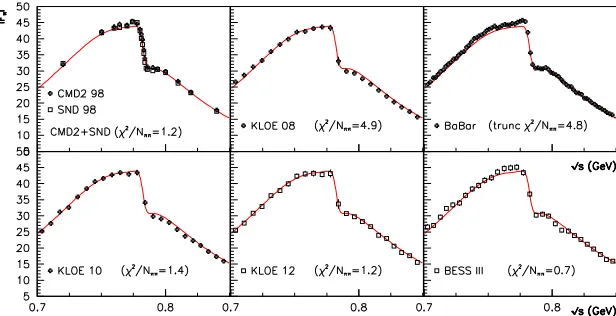
where ˆK(s) is a known kernel function growing form 0.63· · · at the 2mπ threshold to 1 as s→ ∞. The integral is dominated by theρresonance peak shown in figure 3. The experimental errors imply the dominating theoretical uncertainties. As a result I obtain

ahad(1)

Figure 3. A compilation of the modulus square of the pion form factor in theρmeson region, which yields about 75% ofahad

µ . The correspondingR(s) isR(s)= 14β3π|Fπ(0)(s)|2, βπ=

1=4m2π/sis the pion velocity.

0.0 GeV,∞

ρ, ω

1.0 GeV

φ, . . . 2.0 GeV 3.1 GeV

ψ 9.5 GeV

Υ 0.0 GeV,∞

ρ, ω

1.0 GeV

φ, . . . 2.0 GeV

3.1 GeV

∆aµ (δ∆aµ)2

contribution error2

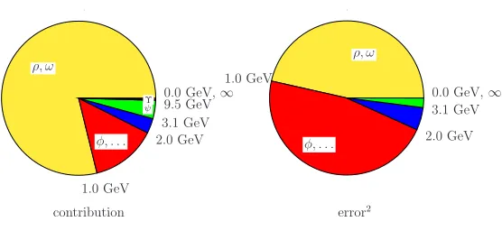
Figure 4.Distribution of contributions and error squares from different energy regions.

Figure 4 shows the distribution of contributions and errors between different energy ranges. One of the main issues isRγ(s) in the region from 1.2 GeV to 2.0 GeV, where more than 30 exclusive channels must be measured and although it contributes about 20% only of the total it contributes about 50% of the uncertainty. In the low energy region, which is particularly important for the dispersive evaluation of the hadronic contribution to the muong₋2, data have improved dramatically in the past decade for the dominante+_e− _{→ π}+_π−_{channel (CMD-2 [12], SND/Novosibirsk [13], KLOE/Frascati [14–16],} BaBar/SLAC [17], BES-III/Beijing [18]) and the statistical errors are a minor problem now. Similarly, the important region between 1.2 GeV to 2.4 GeV has been improved a lot by the BaBar exclusive channel measurements in the ISR mode [19–22]. Recent data sets collected are: e+_e− _{→ 3(π}+_π−_),

e+_e− _{→ pp¯ ande}+_e− _{→ K}0

SKL0,K+K− from CMD-3 [23, 24], and e+e− → nn¯ , e+e− → ηπ+π−, e+_e−_{→ π}0_γ,e+_e−_→ωηπ0_,e+_e−_{→ ωη,e}+_e−_{→ K}+_K−_ande+_e−_→ωπ0 _→π0_π0_{γfrom SND [25–} 27].

Figure 3. A compilation of the modulus square of the pion form factor in theρmeson region, which yields about 75% ofahad

µ . The correspondingR(s) isR(s)=14β3π|Fπ(0)(s)|2, βπ=

1=4m2π/sis the pion velocity.

0.0 GeV,∞

ρ, ω

1.0 GeV

φ, . . . 2.0 GeV 3.1 GeV

ψ 9.5 GeV

Υ 0.0 GeV,∞

ρ, ω

1.0 GeV

φ, . . . 2.0 GeV

3.1 GeV

∆aµ (δ∆aµ)2

contribution error2

Figure 4.Distribution of contributions and error squares from different energy regions.

Figure 4 shows the distribution of contributions and errors between different energy ranges. One of the main issues isRγ(s) in the region from 1.2 GeV to 2.0 GeV, where more than 30 exclusive channels must be measured and although it contributes about 20% only of the total it contributes about 50% of the uncertainty. In the low energy region, which is particularly important for the dispersive evaluation of the hadronic contribution to the muong₋2, data have improved dramatically in the past decade for the dominante+_e− _{→ π}+_π−_{channel (CMD-2 [12], SND/Novosibirsk [13], KLOE/Frascati [14–16],} BaBar/SLAC [17], BES-III/Beijing [18]) and the statistical errors are a minor problem now. Similarly, the important region between 1.2 GeV to 2.4 GeV has been improved a lot by the BaBar exclusive channel measurements in the ISR mode [19–22]. Recent data sets collected are: e+_e− _{→ 3(π}+_π−_),

e+_e− _{→ pp¯ ande}+_e− _{→ K}0

SKL0,K+K− from CMD-3 [23, 24], and e+e− → nn¯ , e+e− → ηπ+π−, e+_e− _→π0_γ,e+_e−_→ωηπ0_,e+_e− _→ωη,e+_e−_{→ K}+_K−_ande+_e−_→ωπ0 _→π0_π0_{γfrom SND [25–} 27].

Above 2 GeV fairly accurate BES-II data [28] are available. Recently, a new inclusive determi-nation ofRγ(s) in the range 1.84 to 3.72 GeV has been obtained with the KEDR detector at Novosi-birsk [29] (see figure 5). A big step in improving low energy cross section measurements has been

Figure 5.Compilation of theR(s) data. New are the KEDR data between 1.84 and 3.72 GeV. Perturbative QCD predictions are also shown.

γ

e

e

γ

hard

s=M2

φ; s′=s(1−k),k=Eγ/Ebeam

π+_π−_{, ρ} 0

φ

b) a)

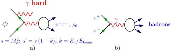
Figure 6.a) Initial state radiation (ISR) on resonance, b) Standard energy scan by tuning the beam energy.

possible with the radiative return or Initial State Radiation (ISR) method figure 6 which has been pioneered by the KLOE Collaboration, followed by BaBar and BES3 experiments. Recent new ex-perimental input for HVP has been obtained by CMD-3 and SND at VEPP-2000 via energy scan and by BESIII at PEPC in the ISR setup (see Contributions by G. Venanzoni, S. Eidelman and A. Denig).

3 NLO and NNLO HVP effects

h e h h h

µ γ

a) b) c)

(a) 3a (b) 3b (c) 3b (d) 3c

(e) 3c (f) 3c (g) 3b,lbl (h) 3d

Figure 7.Feynman diagrams with hadronic insertions at NLO (top row) and NNLO.

the results of an updated evaluation are presented in table 1. The next-to-next leading order (NNLO)

Table 1.NLO contributions diagrams a) - c) (in units 10−11₎

a(2a)

µ a(2µb) a(2µc) ahad(2)µ

-206.13(1.30) 103.49(0.63) 3.37(0.05) -99.27 (0.67)

Table 2.NNLO contributions diagrams (a) - (h) (in units 10−11₎

a(3a)

µ a(3µb) a(3µb,lbl) aµ(3c) a(3µd) ahad(3)µ Ref.

8.0 −4.1 9.1 −0.6 0.005 12.4(1) [31]

7.834 (61) −4.033 (28) 9.005 (63) −0.569 (5) 0.00518 (12) 12.24 (10) [1]

contributions have been calculated recently [31]. Diagrams are shown in figure 7 and corresponding contributions evaluated with kernels from [31] are listed in table 2.

4 News on VP subtraction

(GeV) s 0.6 0.65 0.7 0.75 0.8 0.85 0.9 0.95 1

α

∆

Real

0.03

−

0.02

−

0.01

−

0 0.01 0.02 0.03 0.04 0.05

Exp data

lep

α ∆

=Re

α ∆

Th.pred. for Re

lep+had

α ∆

=Re

α ∆

Th.pred. for Re

Energy (GeV)

0.6 0.65 0.7 0.75 0.8 0.85 0.9 0.95 1

α

∆

Im

0.03 − 0.025 −

0.02 − 0.015 −

0.01 − 0.005 −

0

Exp data

lep α ∆

=Im

α ∆

Th.pred. for Im

lep+had α ∆

=Im

α ∆

Th.pred. for Im

h e h h h

µ γ

a) b) c)

(a) 3a (b) 3b (c) 3b (d) 3c

(e) 3c (f) 3c (g) 3b,lbl (h) 3d

Figure 7.Feynman diagrams with hadronic insertions at NLO (top row) and NNLO.

the results of an updated evaluation are presented in table 1. The next-to-next leading order (NNLO)

Table 1.NLO contributions diagrams a) - c) (in units 10−11₎

a(2a)

µ a(2µb) a(2µc) ahad(2)µ

-206.13(1.30) 103.49(0.63) 3.37(0.05) -99.27 (0.67)

Table 2.NNLO contributions diagrams (a) - (h) (in units 10−11₎

a(3a)

µ a(3µb) a(3µb,lbl) aµ(3c) a(3µd) ahad(3)µ Ref.

8.0 −4.1 9.1 −0.6 0.005 12.4(1) [31]

7.834 (61) −4.033 (28) 9.005 (63) −0.569 (5) 0.00518 (12) 12.24 (10) [1]

contributions have been calculated recently [31]. Diagrams are shown in figure 7 and corresponding contributions evaluated with kernels from [31] are listed in table 2.

4 News on VP subtraction

(GeV) s 0.6 0.65 0.7 0.75 0.8 0.85 0.9 0.95 1

α ∆ Real 0.03 − 0.02 − 0.01 − 0 0.01 0.02 0.03 0.04 0.05 Exp data lep α ∆ =Re α ∆

Th.pred. for Re

lep+had α ∆ =Re α ∆

Th.pred. for Re

Energy (GeV)

0.6 0.65 0.7 0.75 0.8 0.85 0.9 0.95 1

α ∆ Im 0.03 − 0.025 − 0.02 − 0.015 − 0.01 − 0.005 − 0 Exp data lep α ∆ =Im α ∆

Th.pred. for Im

lep+had α ∆ =Im α ∆

Th.pred. for Im

Figure 8.Real and imaginary part of the complex shift∆αof the fine structure constant as measured by KLOE. Reprinted from [33] in Phys. Lett. Bdoi:10.1016/j.physletb.2016.12.016

The first direct measurement of the timelike complex VP function in theρresonance region by

KLOE [33] (see figure 8) nicely confirms dispersion relation calculation and demonstrates the impor-tance of including the imaginary part in vacuum polarization subtraction in obtaining the undressed

σ(0)(s) version of the physical hadronic cross-sectionsσ(s). The complex running fine structure con-stantα(s)= ₁₋α_∆(0)_α(s) is defined in terms of the complex shift∆α(s) =−[Πγ(s)−Πγ(0)]. Measuring

α(s)

α(0) 2

=_σσ₍(_ee++_ee−−_→→_µµ++_µµ−−₎)_pt as well asR(s)=σ(e

+_e−_→π+_π−₎

σ(e+_e−_→µ+_µ−₎, which determines Imα(s)=−α₃R(s), and

know-ing the modulus|α(s)|one can extract Reα(s) as well (see G. Venanzoni’s Contribution fort details).

The imaginary parts in the perturbative regions usually are small relative to the leading logarithms which govern the running couplings (renormalization group approach). In the hadronic shift however, resonances are accompanied by imaginary parts which may be huge in particular near resonances which can decay via OZI suppressed channels only (see Sect. 5 of [1]).

5 Low energy effective Lagrangian theory

Figure 9.Comparing theτ+PDG prediction (red curve) of the pion form factor ine+_e−_{annihilation in theρ−ω} interference region. Reprinted from [7], with kind permission of The European Physical Journal (EPJ).

150 200 250 incl. ISR

DHMZ10 (e+_e−₎

180.2±4.9

[3.6σ]

DHMZ10 (e+_e−_+τ)

189.4±5.4

[2.4σ]

JS11 (e+_e−_+τ)

179.7±6.0

[3.4σ]

HLMNT11 (e+_e−₎

182.8±4.9

[3.3σ]

DHMZ10/JS11 (e+_e−_+τ)

181.1±4.6

[3.6σ]

BDDJ15#_(e+_e−_+τ)

170.4±5.1

[4.8σ]

BDDJ15∗_(e+_e−_+τ)

175.0±5.0

[4.2σ] DHMZ16 (e+_e−₎

181.7±4.2

[3.6σ]

FJ16 (e+_e−_+τ)

177.6±4.4

[4.1σ]

excl. ISR

DHea09 (e+_e−₎

178.8±5.8

[3.5σ]

BDDJ12∗_(e+_e−_+τ)

175.4±5.3

[4.1σ]

experiment

BNL-E821 (world average)

209.1±6.3

aµ×1010-11659000

∗_{HLS global fit}

#_{HLS best fit}

Figure 10. Dependence of aµ predictions on recent evaluations of ahad,LOµ . The HLS best fit BDDJ15#

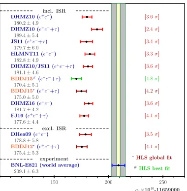
(NSK+KLOE10+KLOE12) does not include BaBar ππdata [39], while BDDJ15∗ _{does. JS11 [40], FJ16 [1]} is updated and includes the BES III and KEDR data. Further points are BDDJ12 [7], DHMZ10 [41], DHMZ16 [22, 44], HLMNT11 [43] and DHea09 [42]. The DHMZ10 (e+_e−_{+τ) result is not including theρ−γ} mixing correction, i.e. it misses important isospin breaking effects. In contrast, DHMZ10/JS11 is obtained by in-cluding this correction, which brings the point into much better agreement with standard analyses based one+_e− data alone, as for example the DHMZ10 (e+_e−_{) result. (see also [21, 45]). Note: results depend on which value} has been taken for HLbL. JS11 and BDDJ13 includes 116(39)×10−11_{[JN] [46], DHea09, DHMZ10, HLMNT11}

and BDDJ12 use 105(26)×10−11_{[PdRV] [47], while FJ16 includes an updated 103(29)×10}−11_.

of HVP by using indirect constraints. The global fit strategy followed in [7] takes into account data belowE0 =1.05GeV (just above theφ) to constrain the effective Lagrangian couplings. Used are 45 different data sets, 6 annihilation channels and 10 partial width decays. The effective theory then allows us to predict cross sections for the channelsπ+_π−_{, π}0_{γ, ηγ, ηγ, π}0_π+_π−_,K+_K−_,K0_K¯0_{, which} account for 83.4% ofahad

µ . The missing channels 4π,5π,6π, ηππ, ωπ and the higher energy tailE>E0 is evaluated using data directly and pQCD for the perturbative region and tail. All mixing effects, as

γρ-mixing,ρω-mixing,· · ·, as well as the decay branching fractions are dynamically generated by including self-energy effects of the spin 1 mesons. One thus is taking into account proper phase space, energy dependent widths etc. Such fit strategy is able to shed light on incompatibilities in the data, e.g. KLOE vs BaBar, by comparing the fit qualities, but also reveals the compatibility ofτ–decay spectra withe+_e−_{–data after accounting for the mixing effects like includingγ−ρ}0_{mixing. HLS estimates} are included in table 10 together with other recent results.

6 HVP from lattice QCD (following H. Wittig at LATTICE 2016)

The need for ab initio calculation of ahad

150 200 250 incl. ISR

DHMZ10 (e+_e−₎

180.2±4.9

[3.6σ]

DHMZ10 (e+_e−_+τ)

189.4±5.4

[2.4σ]

JS11 (e+_e−_+τ)

179.7±6.0

[3.4σ]

HLMNT11 (e+_e−₎

182.8±4.9

[3.3σ]

DHMZ10/JS11 (e+_e−_+τ)

181.1±4.6

[3.6σ]

BDDJ15#_(e+_e−_+τ)

170.4±5.1

[4.8σ]

BDDJ15∗_(e+_e−_+τ)

175.0±5.0

[4.2σ] DHMZ16 (e+_e−₎

181.7±4.2

[3.6σ]

FJ16 (e+_e−_+τ)

177.6±4.4

[4.1σ]

excl. ISR

DHea09 (e+_e−₎

178.8±5.8

[3.5σ]

BDDJ12∗_(e+_e−_+τ)

175.4±5.3

[4.1σ]

experiment

BNL-E821 (world average)

209.1±6.3

aµ×1010-11659000

∗_{HLS global fit}

#_{HLS best fit}

Figure 10. Dependence of aµ predictions on recent evaluations of ahad,LOµ . The HLS best fit BDDJ15#

(NSK+KLOE10+KLOE12) does not include BaBar ππdata [39], while BDDJ15∗ _{does. JS11 [40], FJ16 [1]} is updated and includes the BES III and KEDR data. Further points are BDDJ12 [7], DHMZ10 [41], DHMZ16 [22, 44], HLMNT11 [43] and DHea09 [42]. The DHMZ10 (e+_e−_{+τ) result is not including theρ−γ} mixing correction, i.e. it misses important isospin breaking effects. In contrast, DHMZ10/JS11 is obtained by in-cluding this correction, which brings the point into much better agreement with standard analyses based one+_e− data alone, as for example the DHMZ10 (e+_e−_{) result. (see also [21, 45]). Note: results depend on which value} has been taken for HLbL. JS11 and BDDJ13 includes 116(39)×10−11_{[JN] [46], DHea09, DHMZ10, HLMNT11}

and BDDJ12 use 105(26)×10−11_{[PdRV] [47], while FJ16 includes an updated 103(29)×10}−11_.

of HVP by using indirect constraints. The global fit strategy followed in [7] takes into account data belowE0 =1.05GeV (just above theφ) to constrain the effective Lagrangian couplings. Used are 45 different data sets, 6 annihilation channels and 10 partial width decays. The effective theory then allows us to predict cross sections for the channelsπ+_π−_{, π}0_{γ, ηγ, ηγ, π}0_π+_π−_,K+_K−_,K0_K¯0_{, which} account for 83.4% ofahad

µ . The missing channels 4π,5π,6π, ηππ, ωπ and the higher energy tailE>E0 is evaluated using data directly and pQCD for the perturbative region and tail. All mixing effects, as

γρ-mixing,ρω-mixing,· · ·, as well as the decay branching fractions are dynamically generated by including self-energy effects of the spin 1 mesons. One thus is taking into account proper phase space, energy dependent widths etc. Such fit strategy is able to shed light on incompatibilities in the data, e.g. KLOE vs BaBar, by comparing the fit qualities, but also reveals the compatibility ofτ–decay spectra withe+_e−_{–data after accounting for the mixing effects like includingγ−ρ}0_{mixing. HLS estimates} are included in table 10 together with other recent results.

6 HVP from lattice QCD (following H. Wittig at LATTICE 2016)

The need for ab initio calculation of ahad

µ is well motivated: – the problems to determine non-perturbative contributions to the muong−2 from experimental data at sufficient precision persists and is not easy to improve, – a model–independent extension of CHPT to the relevant energies ranges up to 2 GeV is missing, while the new experiments E989 FNAL and E34 J-PARC require an im-provement of the hadronic uncertainties by a factor two to four.

The hope is that LQCD can deliver estimates of accuracy

δaHVPµ /aHVPµ <0.5%, δaHLbLµ /aHLbLµ 10% (3)

in the coming years.

Primary object for getting HVP in LQCD is the e.m. current correlator in configuration space

Jµ(x,t)Jν(0,0); Jµ=2

3u¯γµu−1

3d¯γµd−1

3s¯γµs+· · · (4)

In principle, a Fourier transform

Πµν(Q)=

d4xei QxJµ(x) Jν(0)=

QµQν−δµνQ2

Π(Q2) (5)

yields the vacuum polarization functionΠ(Q2_{) needed to calculate}

aHVP µ =4α2

∞

0 dQ

2_f(Q2_)Π(Q2_{)−Π(0) . (6)}

The integration kernel in this representation is

f(Q2_)=w(Q2_/m2

µ)/Q2; w(r)=

16

r2₁₊ √_1+4/r4 √_1+4/r . (7)

As LQCD per se has to work on a lattice in a finite box, momenta are quantizedQmin=2π/L, where

−Π(Q2₎

Pad´e

approx. numerical

interpolation of lattice data

pQCD

≈0.1 GeV2 _{≈4 GeV}2

Q2 × × × × × × × × × × × × × × × × × × × × × × ×× × × × × × × × × × × × × × × × × × × × × × × ××

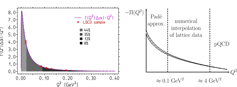
Figure 11. Left: the integrand of (6) as a function of Q2_{. Also shown are ranges between Q}

i =

0.00,0.15,0.30,0.45 and 1.0GeV and their percent contribution toahad

µ and a possible “LQCD sample”. Right:

typical ranges for lattice data and their extrapolation to lowQ2_.

Lis the lattice box length. Therefore, approaching low momentaQmin → 0 ⇔ L → ∞requires a sufficiently large volume. Present state of the art calculations reachQ_min=2π/LwithmπaL4 for

mπ ∼200MeV, such thatQmin ∼314MeV. This means that about 44% of the lowQcontribution to

ahad

µ is not covered by data yet. Typically, lattice data are available forQ2 >(2π/L)2, which one has to extrapolate toQ2_{=0 by VMD type modeling [48] or via Padé’s [49] or analytic continuation [51].} The method requires a reliable estimate of the bareΠ(0) (see e.g. [50]). In order to reach the required accuracy one needs LQCD data down toQ2

600 650 700 750 800 Nf=2+1+1

■ HPQCD 16

666±13

■ ETM 15

678±29

■ ETM 13

674±28 Nf=2+1

▲ RBC/UKQCD 11

641±46

▲ Aubin+Blum 07

748±21

▲ Aubin+Blum 07

713±15 Nf=2

■ Mainz/CLS 16

652±35

▲ Mainz/CLS 11

618±64

❙ ETM 11

572±16

e+_e−_&τdata

688.77±3.38

aHVP

µ ·1010

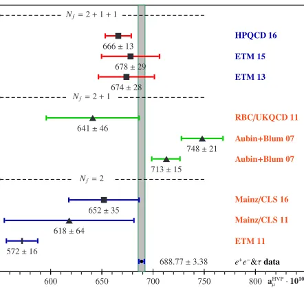
Figure 12. Summary of recent LQCD results for the leading orderaHVP

µ , in units 10−10. Labels: marks u,d,s,c,u,d,sandu,dcontributions. Individual flavor contributions from light (u,d) amount to about 90%, strange about 8% and charm about 2%. Results shown are from HPQCD 16 [56], ETM 15 [57], ETM 13 [58], RBC/UKQCD 11 [52], Aubin+Blum 07 [59], Mainz/CLS 16 [60], Mainz/CLS 11 [61] and ETM 11 [48]. The vertical band shows thee+_e−_{data driven DR estimate (2).}

7 Alternative method to get

a

µ

: using

α

(

t

=

−

Q

)

measured via

t

–channel

exchange processes.

A promising alternative method to determineahad

µ is possible by a dedicated measurement ofα(t) at spacelike momentum transfer as advocated in [62] and [63]. Givenα(−Q2_{) and the fact that the} leptonic contribution is well under control in perturbation theory one can extract the hadronic shift

∆αhad(−Q2₎₌₁₋ α

α(−Q2₎−∆αlep(−Q2) (8)

and determineahad

µ via the representation

ahad µ =

α π

1

0

dx (1−x)∆αhad−Q2_{(x) (9)}

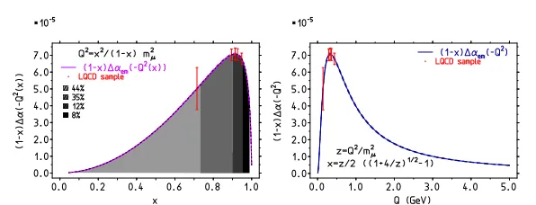
whereQ2_(x)≡ x2

1−xm2µis the spacelike square momentum–transfer. In the Euclidean region the inte-grand is highly peaked around half of theρmeson mass scale (see figure 13). The method is very

600 650 700 750 800 Nf=2+1+1

■ HPQCD 16

666±13

■ ETM 15

678±29

■ ETM 13

674±28 Nf=2+1

▲ RBC/UKQCD 11

641±46

▲ Aubin+Blum 07

748±21

▲ Aubin+Blum 07

713±15 Nf=2

■ Mainz/CLS 16

652±35

▲ Mainz/CLS 11

618±64

❙ ETM 11

572±16

e+_e−_&τdata

688.77±3.38

aHVP

µ ·1010

Figure 12. Summary of recent LQCD results for the leading orderaHVP

µ , in units 10−10. Labels: marks u,d,s,c,u,d,sandu,dcontributions. Individual flavor contributions from light (u,d) amount to about 90%, strange about 8% and charm about 2%. Results shown are from HPQCD 16 [56], ETM 15 [57], ETM 13 [58], RBC/UKQCD 11 [52], Aubin+Blum 07 [59], Mainz/CLS 16 [60], Mainz/CLS 11 [61] and ETM 11 [48]. The vertical band shows thee+_e−_{data driven DR estimate (2).}

7 Alternative method to get

a

µ

: using

α

(

t

=

−

Q

)

measured via

t

–channel

exchange processes.

A promising alternative method to determineahad

µ is possible by a dedicated measurement ofα(t) at spacelike momentum transfer as advocated in [62] and [63]. Givenα(−Q2_{) and the fact that the} leptonic contribution is well under control in perturbation theory one can extract the hadronic shift

∆αhad(−Q2₎₌₁₋ α

α(−Q2₎−∆αlep(−Q2) (8)

and determineahad

µ via the representation

ahad µ = α π 1 0

dx (1−x)∆αhad−Q2_{(x) (9)}

whereQ2_(x)≡ x2

1−xm2µis the spacelike square momentum–transfer. In the Euclidean region the inte-grand is highly peaked around half of theρmeson mass scale (see figure 13). The method is very

different from the standard approach based on (1): radiative corrections are very different (much sim-pler) as no hadronic final states need to be understood, no VP subtraction is to be performed, no exclusive channel collection etc. So, even a 1% level measurement can provide important indepen-dent information. This in view of the problem to get accurate hadronic total cross–section in the range

Figure 13.The integrand of theahad

µ integral (9) as functions ofxandQis strongly peaked at about 330MeV.

Legend as in figure 11.

between 1 and 2 GeV and possible unsettled problems (non-convergence of the Dyson resummation near OZI suppressed resonances) in VP subtraction as addressed recently in Sect. 5 of [1].

The possible processes to measureα(t) are Bhabha scatteringe+_{(p+) e}−_(p

−) → e+(p+) e−(p−) or muon electron scattering (see figure 14). The Bhabha process has two tree level diagrams at– and

γ _↑t

e− e+ e− e+ γ → s

e− _e− e+

e+ +

γ ↑t

e′ µ′

e

µ

Figure 14.Measuring the running charge in the spacelike regime. Left: VP dressed tree level Bhabha scattering in QED, for smallt(small angels) theschannel is suppressed. Right: gettingα(t) from theµ−_e−_→µ−_e−_process.

as–channel one. With the positive c.m. energy square s=(p++p−)2and the negative momentum transfer squaret=(p₋−p₋)2=−1₂(s−4m2_e) (1−cosθ), θthee−_{scattering angle, there are two very} different scales involved which helps to isolate thetchannel of interest. The VP dressed lowest order cross–section is

dσ

d cosΘ =

s

48π

ik|Aik|

2_{, (10)}

whereAikare tree level helicity amplitudes,i,k=L,R denote left– and right–handed electrons. The dressed transition amplitudes in the massless limit (me≈0 ) read

|ALL,RR|2 =3₈ (1+cosθ)2

e

2_(s)

s +

e2_(t)

t

2

; |ALR,RL|2=3₈ (1−cosθ)2

e

2_(s)

s +

e2_(t)

t 2 . (11)

Preferably one uses small angle Bhabha scattering (small|t|) as a normalizing process which is dom-inated by thet–channel∼1/t, however, detecting electrons and positrons along the beam axis often

has its technical limitations. Care also is needed concerning the ISR corrections because cuts for the Bhabha process (e+_e−→e+_{e−) typically are different from the ones applied to e}+_{e−→hadrons.}

While the Bhabha process requires to sort out theschannel from thetchannel, the puretchannel reaction ofµ−e−scatteringµ−(p−) e−(q−)→µ−(p−)e−(q−) provides a much simpler setup and could be realized as a fixed target experiment [63] at existing facilities. The leading order cross–section in this case has the simple form

dσunpol_µ−_e−_→.µ−_e−

dt =4π α(t)2 1

λ(s,m2

e,m2µ)

  

s−m2 µ−m2e

2

t2 +

s t +

1 2

 

, (12)

exhibiting the effective charge as an overall factor. For details see Luca Trentadue’s Contribution. Such an experiment would provide data for the Euclidean electromagnetic current correlatorΠγ(Q2)− Π_γ(0) = ₋∆αhad(−Q2_{) =} α

α(−Q2₎ + ∆αlep(−Q2)−1 and would allow for a directly check of lattice

QCD data. In addition one could determine∆αhad−Q2_{atQ≈2.5GeV by this method (one single} number!) as the non-perturbative part of∆αhadM2

Z

= ∆αhad−Q2_{+pert. when evaluated in “Adler} function” approach advocated in [64].

8 Theory confronts experiment

Table 3.Standard model theory and experiment comparison [in units 10−10_].

Contribution Value Error Reference

QED incl. 4-loops+5-loops 11 658 471 . 8851 0 . 036 Remiddi, Kinoshita et al.

Leading hadronic vac. pol. 688 . 77 3 . 38 data-drivene+_e−_+τ

Subleading hadronic vac. pol. -9 . 927 0 . 072 2016 update

NNLO hadronic vac. pol. 1 . 224 0 . 010 [31]

Hadronic light–by–light 10 . 34 2 . 88 [46, 69]

Weak incl. 2-loops 15 . 36 0 . 11 [11, 70]

Theory 11 659 177 . 6 4 . 4 –

Experiment 11 659 209 . 1 6 . 3 [2] updated

Exp.- The. 4.1 standard deviations 31 . 3 7 . 7 –

Table 3 summarizes the present status of the SM prediction foraµ in comparison with the ex-perimental value [2]. For a recent update of the weak contribution see [70]. As an estimate based on [4–6, 10, 46, 65, 68, 69] we adoptπ0, η, η[95±12]+axial–vector [8± 3]+scalar [−6± 1]+

π,Kloops [−20±5]+quark loops [22± 4]+tensor [1± 0]+NLO [3± 2] which yields

a(6)

µ (lbl,had)=(103±29)×10−11. (13)

While the Bhabha process requires to sort out theschannel from thetchannel, the puretchannel reaction ofµ−e−scatteringµ−(p−) e−(q−)→µ−(p−)e−(q−) provides a much simpler setup and could be realized as a fixed target experiment [63] at existing facilities. The leading order cross–section in this case has the simple form

dσunpol_µ−_e−_→.µ−_e−

dt =4π α(t)2 1

λ(s,m2

e,m2µ)

  

s−m2 µ−m2e

2

t2 +

s t +

1 2

 

, (12)

exhibiting the effective charge as an overall factor. For details see Luca Trentadue’s Contribution. Such an experiment would provide data for the Euclidean electromagnetic current correlatorΠγ(Q2)− Π_γ(0) = ₋∆αhad(−Q2_{) =} α

α(−Q2₎ + ∆αlep(−Q2)−1 and would allow for a directly check of lattice

QCD data. In addition one could determine∆αhad−Q2_{atQ≈2.5GeV by this method (one single} number!) as the non-perturbative part of∆αhadM2

Z

= ∆αhad−Q2_{+pert. when evaluated in “Adler} function” approach advocated in [64].

8 Theory confronts experiment

Table 3.Standard model theory and experiment comparison [in units 10−10_].

Contribution Value Error Reference

QED incl. 4-loops+5-loops 11 658 471 . 8851 0 . 036 Remiddi, Kinoshita et al.

Leading hadronic vac. pol. 688 . 77 3 . 38 data-drivene+_e−_+τ

Subleading hadronic vac. pol. -9 . 927 0 . 072 2016 update

NNLO hadronic vac. pol. 1 . 224 0 . 010 [31]

Hadronic light–by–light 10 . 34 2 . 88 [46, 69]

Weak incl. 2-loops 15 . 36 0 . 11 [11, 70]

Theory 11 659 177 . 6 4 . 4 –

Experiment 11 659 209 . 1 6 . 3 [2] updated

Exp.- The. 4.1 standard deviations 31 . 3 7 . 7 –

Table 3 summarizes the present status of the SM prediction foraµin comparison with the ex-perimental value [2]. For a recent update of the weak contribution see [70]. As an estimate based on [4–6, 10, 46, 65, 68, 69] we adoptπ0, η, η[95±12]+axial–vector [8± 3]+scalar [−6± 1]+

π,Kloops [−20±5]+quark loops [22± 4]+tensor [1± 0]+NLO [3± 2] which yields

a(6)

µ (lbl,had)=(103±29)×10−11. (13)

The result differs little from the “agreed” value (105±26)×10−11 _{presented in [47] and (116±} 39)×10−11 _{estimated in [46]. Both included a wrong, too large, Landau-Yang theorem violating} axial–vector contribution from [10], correcting for this we obtain our reduced value relative to [46].

The following tabular collects recent new/updated evaluations:

New contribution Reference ∆aµ·1011

NNLO HVP Kurz et al. 2014 12.4 ± 0.1

NLO HLbL Colangelo et al. 2014 3 ± 2

New axial exchange HLbL Pauk, Vanderhaeghen [66], FJ14 [1, 67] 7.55 ± 2.71

Tensor exchange HLbL Pauk, Vanderhaeghen 2014 1.1 ± 0.1

Newπ0exchange HLbL π0γ∗_γ∗_{constraint from LQCD [68] 64.68 ± 12.40}

· · · ·

Old axial exchange HLbL Melnikov, Vainshtein 2004 22 ± 5

Oldπ0exchange HLbL JN [46] 72 ± 12

Total change −5.6 ± 12.85 [←13]

The uncertainty from these contributions remains unchanged, while the central value is shifted downwards by almost 1 SD.

Possible interpretations of the 4σdeviation: new physics?, a statistical fluctuation?, underesti-mated uncertainties (experimental, theoretical)? Do experiments measure what theoreticians calcu-late? The challenge for the future is to keep up with the future experiments, which will improve the experimental accuracy fromδaexpµ =63×10−11[±0.54 ppm] at present toδaexpµ =16×10−11[±0.14 ppm] the next years. Next generation experiments require a factor 4 reduction of the uncertainty optimistically feasible should be a factor 2 we hope.

In view of the upcoming twocomplementaryexperiments, one at Fermilab working with ultra hot muons and the other at J-PARC operating with ultra cold muons (very different radiation effects), the big challenge is to keep up on the prediction side as much as possible. The deviation between theory and experiment can be scrutinized provided theory and the needed cross section data improves the same as the muong−2 experiments. Primarily we need more/better data and/or progress in non-perturbative QCD, where the main obstacle (data, lattice QCD, RLA) is the hadronic light-by-light scattering contribution. Progress in evaluating HVP also depends on more data (BaBar, Belle, VEPP-2000, BESIII,...) and lattice QCD where recent progress is very promising (see figure 12). In both cases HVP as well as HLbL, lattice QCD will provide answers one day, but also low energy effective RL and DR approaches need be further developed. One has also to keep in mind that progress in calculations of radiative corrections [71–73] is mandatory in precision measurements of hadronic cross sections.

For future improvements of HLbL one urgently needs more information from γγ _→ hadrons physics [74, 75] in order to have better constraints on modeling hadronic amplitudes (see [76–78] for theoretical studies). Some sample processes are collected in figure 15. Mostly experiments ate+_e−_–

e+

e−

P, V, Sqq¯

π¯π, KK, T, S¯ qqq¯q¯

γ

γ

e+

e− P

γ

γ γ

γ

e+

e−

P γ

γ V

e+

e−

P γ

γ V

e+_e−

facilities investigate single-tag events (higher rates, lower background). New data are expected from KLOE, KEDR exhibiting taggers and from BaBar, Belle, BES III which have high luminosity. More information is also expected from Dalitz–decay studiesρ, ω, φ_→π0(η)e+_e−_{possible at Novosibirsk,} CERN NA60, JLab, Mainz, Bonn, Jülich and BES. Unfortunately some of the interesting processes seem to be buried in the background. The background is a general problem inγγ_→hadrons physics. The dispersive approach [8, 66] is able to allow for real progress since contributions which we have treated so far as separate contributions will be treated in an integral manner. An example is the

γγ → ππprocess which includes contributions attributed to the two–pion channel , the pion–loop, the scalar contribution as well as the tensor contribution. All-in-one can be gotten from the experi-mental data (see e.g. figure 3 of [79]). This also will settle such issues as the pion polarizability. A lot remains to be done while newaexpµ is expected soon. For details see the Contribution by M. Procura.

Thanks to the organizers for the kind invitation and support to the “KLOE-2 Workshop one+_e−_{collision physics} at 1 GeV” at Frascati, and for giving me the opportunity to present this talk.

References

[1] F. Jegerlehner, EPJ Web Conf.118, 01016 (2016)

[2] G. W. Bennett et al. [Muon g-2 Collaboration], Phys. Rev. D73, 072003 (2006) [3] D. W. Hertzog, EPJ Web Conf.118, 01015 (2016)

[4] M. Hayakawa, T. Kinoshita, A. I. Sanda, Phys. Rev. Lett.75, 790 (1995); Phys. Rev. D54, 3137 (1996); M. Hayakawa, T. Kinoshita, Phys. Rev. D 57, 465 (1998) [Erratum-ibid. D66, 019902 (2002)];

[5] J. Bijnens, E. Pallante, J. Prades, Phys. Rev. Lett. 75, 1447 (1995) [Erratum-ibid. 75, 3781 (1995)]; Nucl. Phys. B474, 379 (1996); [Erratum-ibid.626, 410 (2002)];

J. Bijnens, J. Prades, Mod. Phys. Lett. A22, 767 (2007) [6] M. Knecht, A. Nyffeler, Phys. Rev. D65, 073034 (2002)

[7] M. Benayoun, P. David, L. DelBuono, F. Jegerlehner, Eur. Phys. J. C72, 1848 (2012);73, 2453 (2013)

[8] G. Colangelo et al., Phys. Lett. B738, 6 (2014)

[9] M. Knecht, S. Peris, M. Perrottet, E. de Rafael, JHEP0211, 003 (2002) [10] K. Melnikov, A. Vainshtein, Phys. Rev. D70, 113006 (2004)

[11] A. Czarnecki, W. J. Marciano, A. Vainshtein, Phys. Rev. D67, 073006 (2003) [Erratum-ibid. D 73, 119901 (2006)]

[12] R. R. Akhmetshin et al. [CMD-2 Collab.], Phys. Lett. B578, 285 (2004); V. M. Aulchenko et al. [CMD-2 Collab.], JETP Lett.82, 743 (2005) [Pisma Zh. Eksp. Teor. Fiz.82, 841 (2005)]; R. R. Akhmetshin et al., JETP Lett.84, 413 (2006) [Pisma Zh. Eksp. Teor. Fiz.84, 491 (2006)]; Phys. Lett. B648, 28 (2007)

[13] M. N. Achasov et al. [SND Collab.], J. Exp. Theor. Phys.103, 380 (2006) [Zh. Eksp. Teor. Fiz. 130, 437 (2006)]

[14] A. Aloisio et al. [KLOE Collab.], Phys. Lett. B606, 12 (2005); F. Ambrosino et al. [KLOE Collab.], Phys. Lett. B670, 285 (2009)

[15] F. Ambrosino et al. [KLOE Collab.], Phys. Lett. B700, 102 (2011) [16] D. Babusci et al. [KLOE Collab.], Phys. Lett. B720, 336 (2013)

facilities investigate single-tag events (higher rates, lower background). New data are expected from KLOE, KEDR exhibiting taggers and from BaBar, Belle, BES III which have high luminosity. More information is also expected from Dalitz–decay studiesρ, ω, φ_→π0(η)e+_e−_{possible at Novosibirsk,} CERN NA60, JLab, Mainz, Bonn, Jülich and BES. Unfortunately some of the interesting processes seem to be buried in the background. The background is a general problem inγγ_→hadrons physics. The dispersive approach [8, 66] is able to allow for real progress since contributions which we have treated so far as separate contributions will be treated in an integral manner. An example is the

γγ → ππprocess which includes contributions attributed to the two–pion channel , the pion–loop, the scalar contribution as well as the tensor contribution. All-in-one can be gotten from the experi-mental data (see e.g. figure 3 of [79]). This also will settle such issues as the pion polarizability. A lot remains to be done while newaexpµ is expected soon. For details see the Contribution by M. Procura.

Thanks to the organizers for the kind invitation and support to the “KLOE-2 Workshop one+_e−_{collision physics} at 1 GeV” at Frascati, and for giving me the opportunity to present this talk.

References

[1] F. Jegerlehner, EPJ Web Conf.118, 01016 (2016)

[2] G. W. Bennett et al. [Muon g-2 Collaboration], Phys. Rev. D73, 072003 (2006) [3] D. W. Hertzog, EPJ Web Conf.118, 01015 (2016)

[4] M. Hayakawa, T. Kinoshita, A. I. Sanda, Phys. Rev. Lett.75, 790 (1995); Phys. Rev. D54, 3137 (1996); M. Hayakawa, T. Kinoshita, Phys. Rev. D 57, 465 (1998) [Erratum-ibid. D66, 019902 (2002)];

[5] J. Bijnens, E. Pallante, J. Prades, Phys. Rev. Lett. 75, 1447 (1995) [Erratum-ibid. 75, 3781 (1995)]; Nucl. Phys. B474, 379 (1996); [Erratum-ibid.626, 410 (2002)];

J. Bijnens, J. Prades, Mod. Phys. Lett. A22, 767 (2007) [6] M. Knecht, A. Nyffeler, Phys. Rev. D65, 073034 (2002)

[7] M. Benayoun, P. David, L. DelBuono, F. Jegerlehner, Eur. Phys. J. C72, 1848 (2012);73, 2453 (2013)

[8] G. Colangelo et al., Phys. Lett. B738, 6 (2014)

[9] M. Knecht, S. Peris, M. Perrottet, E. de Rafael, JHEP0211, 003 (2002) [10] K. Melnikov, A. Vainshtein, Phys. Rev. D70, 113006 (2004)

[11] A. Czarnecki, W. J. Marciano, A. Vainshtein, Phys. Rev. D67, 073006 (2003) [Erratum-ibid. D 73, 119901 (2006)]

[12] R. R. Akhmetshin et al. [CMD-2 Collab.], Phys. Lett. B578, 285 (2004); V. M. Aulchenko et al. [CMD-2 Collab.], JETP Lett.82, 743 (2005) [Pisma Zh. Eksp. Teor. Fiz.82, 841 (2005)]; R. R. Akhmetshin et al., JETP Lett.84, 413 (2006) [Pisma Zh. Eksp. Teor. Fiz.84, 491 (2006)]; Phys. Lett. B648, 28 (2007)

[13] M. N. Achasov et al. [SND Collab.], J. Exp. Theor. Phys.103, 380 (2006) [Zh. Eksp. Teor. Fiz. 130, 437 (2006)]

[14] A. Aloisio et al. [KLOE Collab.], Phys. Lett. B606, 12 (2005); F. Ambrosino et al. [KLOE Collab.], Phys. Lett. B670, 285 (2009)

[15] F. Ambrosino et al. [KLOE Collab.], Phys. Lett. B700, 102 (2011) [16] D. Babusci et al. [KLOE Collab.], Phys. Lett. B720, 336 (2013)

[17] B. Aubert et al. [BABAR Collab.], Phys. Rev. Lett. 103, 231801 (2009); J. P. Lees et al., Phys.Rev.D86, 032013 (2012)

[18] M. Ablikim et al. [BESIII Collab.], Phys. Lett. B753, 629 (2016)

[19] B. Aubert et al. [BABAR Collab.], Phys. Rev. D70, 072004 (2004); 71, 052001 (2005); 73, 012005 (2006);73, 052003 (2006);76, 012008, ibid. 092005, ibid. 092006, (2007);77, 092002 (2008)

[20] J. P. Lees et al. [BaBar Collab.], Phys. Rev. D85, 112009 (2012);86, 012008 (2012);87, 092005 (2013);88, 032013 (2013);89, 092002 (2014)

[21] M. Davier, Nucl. Part. Phys. Proc.260, 102 (2015)

[22] M. Davier, A. Höcker, B. Malaescu, Z. Zhang, Adv. Ser. Direct. High Energy Phys.26, 129 (2016)

[23] R. R. Akhmetshin et al. [CMD-3 Collaboration], Phys. Lett. B723, 82 (2013);759, 634 (2016) [24] E. A. Kozyrev et al. [CMD-3 Collaboration], Phys. Lett. B760, 314 (2016)

[25] M. N. Achasov et al., Phys. Rev. D90, no.11, 112007 (2014)

[26] V. M. Aulchenko et al. [SND Collaboration], Phys. Rev. D91, no.5, 052013 (2015)

[27] M. N. Achasov et al. [SND Collaboration], Phys. Rev. D93, no.9, 092001 (2016); 94, no.3, 032010 (2016);94, no.9, 092002 (2016);94, no.11, 112006 (2016);94, no.11, 112001 (2016) [28] J. Z. Bai et al. [BES Collab.], Phys. Rev. Lett.84, 594 (2000); Phys. Rev. Lett. 88, 101802

(2000); M. Ablikim et al., Phys. Lett. B677, 239 (2009)

[29] V. V. Anashin et al., Phys. Lett. B753, 533 (2016); arXiv:1610.02827 [hep-ex]. [30] B. Krause, Phys. Lett. B390, 392 (1997)

[31] A. Kurz, T. Liu, P. Marquard, M. Steinhauser, Phys.Lett.B734, 144 (2014) [32] G. Colangelo et al., Phys.Lett.B735, 90 (2014)

[33] A. Anastasi et al. [KLOE-2 Collaboration], doi:10.1016/j.physletb.2016.12.016 arXiv:1609.06631 [hep-ex].

[34] R. Barate et al. [ALEPH Collab.], Z. Phys. C76, 15 (1997); Eur. Phys. J. C4, 409 (1998); S. Schael et al. [ALEPH Collab.], Phys. Rept.421, 191 (2005)

[35] M. Davier et al., Eur.Phys.J.C74, 2803 (2014)

[36] K. Ackerstaffet al. [OPAL Collab.], Eur. Phys. J. C7, 571 (1999) [37] S. Anderson et al. [CLEO Collab.], Phys. Rev. D61, 112002 (2000) [38] M. Fujikawa et al. [Belle Collab.], Phys. Rev. D78, 072006 (2008)

[39] M. Benayoun, P. David, L. DelBuono, F. Jegerlehner, Eur. Phys. J. C75, no.12, 613 (2015) [40] F. Jegerlehner, R. Szafron, Eur. Phys. J. C71, 1632 (2011)

[41] M. Davier, A. Höcker, B. Malaescu, Z. Zhang, Eur. Phys. J. C71, 1515 (2011) [Erratum-ibid. C 72, 1874 (2012)]

[42] M. Davier et al., Eur. Phys. J. C66, 127 (2010)

[43] K. Hagiwara, R. Liao, A. D. Martin, D. Nomura, T. Teubner, J. Phys. G G38, 085003 (2011) [44] M. Davier, arXiv:1612.02743 [hep-ph].

[45] Z. Zhang, EPJ Web Conf.118, 01036 (2016) doi:10.1051/epjconf/201611801036 [46] F. Jegerlehner, A. Nyffeler, Phys. Rept.477, 1 (2009)

[47] J. Prades, E. de Rafael, A. Vainshtein, Adv. Ser. Direct. High Energy Phys.20, 303 (2009) [48] X. Feng, K. Jansen, M. Petschlies, D. B. Renner, Phys. Rev. Lett.107, 081802 (2011) [49] M. Golterman, K. Maltman, S. Peris, Phys. Rev. D90, no.7, 074508 (2014)

[50] S. Borsanyi et al., arXiv:1612.02364 [hep-lat]. [51] X. Feng et al., Phys. Rev. D88, 034505 (2013)

[54] A. Francis et al., arXiv:1411.3031 [hep-lat]

[55] R. Malak et al. [Budapest-Marseille-Wuppertal Collab.], PoS LATTICE2014, 161 (2015) [56] B. Chakraborty, C. T. H. Davies, P. G. de Oliviera, J. Koponen, G. P. Lepage, arXiv:1601.03071

[hep-lat].

[57] F. Burger, X. Feng, K. Jansen, M. Petschlies, G. Pientka, D. B. Renner, EPJ Web Conf.118, 01029 (2016)

[58] F. Burger et al. [ETM Collab.], JHEP1402, 099 (2014) [59] C. Aubin, T. Blum, Phys. Rev. D75, 114502 (2007)

[60] M. Della Morte, G. Herdoiza, H. Horch, B. Jäger, H. Meyer, H. Wittig, PoS LATTICE2015, 111 (2015) [arXiv:1602.03976 [hep-lat]]

[61] M. Della Morte, B. Jäger, A. Jüttner, H. Wittig, JHEP1203, 055 (2012)

[62] C. M. Carloni Calame, M. Passera, L. Trentadue, G. Venanzoni, Phys. Lett. B746, 325 (2015) [63] G. Abbiendi et al., arXiv:1609.08987 [hep-ex]

[64] F. Jegerlehner, Nucl. Phys. Proc. Suppl.181-182, 135 (2008);Hadronic effects in(g−2)µand

αQED(MZ): Status and perspectives, In: Radiative Corrections, ed by J. Solà (World Scientific, Singapore 1999) pp 75–89 [hep-ph/9901386].

[65] A. Nyffeler, EPJ Web Conf.118, 01024 (2016)

[66] V. Pauk, M. Vanderhaeghen, Eur. Phys. J. C74, 3008 (2014)

[67] F. Jegerlehner, Talk at the MITP Workshop “Hadronic contributions to the muon anomalous magnetic moment”, 1-5 April 2014, Waldthausen Castle near Mainz,

[68] A. Gérardin, H. B. Meyer, A. Nyffeler, arXiv:1607.08174 [hep-lat] [69] J. Bijnens, J. Relefors, arXiv:1608.01454 [hep-ph].

[70] C. Gnendiger, D. Stöckinger, H. Stöckinger-Kim, Phys. Rev. D88, 053005 (2013) [71] S. Actis et al., Eur. Phys. J. C66, 585 (2010)

[72] H. Czy˙z, Int. J. Mod. Phys. Conf. Ser.35, 1460402 (2014) doi:10.1142/S2010194514604025 [73] F. Jegerlehner, K. Kołodziej, arXiv:1701.01837 [hep-ph].

[74] D. Babusci et al., Eur. Phys. J. C72, 1917 (2012)

[75] A. Nyffeler, PoS CD12, 045 (2013) [arXiv:1306.5987 [hep-ph]] [76] G. Mennessier, Z. Phys. C16, 241 (1983)

[77] B. Moussallam, Eur. Phys. J. C73, 2539 (2013)