Simulation Software Selection using Principal
Component Analysis
Dr. Ashu Gupta
Assistant Professor, Department of Computer Science, College of Arts & Sciences, Prince Sattam Bin Abdulaziz
University, Wadi Al-Dawasir, Saudi Arabia
ABSTRACT: In a period of continuous change in global business environment, organizations, large and small, are finding it increasingly difficult to deal with, and adjust to the demands for such change. Simulation is a powerful stool for allowing designers imagine new systems and enabling them to both quantify and observe behavior. Currently the market offers a variety of simulation software packages. Some are less expensive than others. Some are generic and can be used in a wide variety of application areas while others are more specific. Some have powerful features for modeling while others provide only basic features. Modeling approaches and strategies are different for different packages. Companies are seeking advice about the desirable features of software for manufacturing simulation, depending on the purpose of its use. Because of this, the importance of an adequate approach to simulation software evaluation and selection is apparent. This paper presents an application of Principal Component Analysis for Simulation Software Selection.
KEYWORDS: Simulation, Simulation software, Evaluation, Selection
I. INTRODUCTION
Growing competition in many industries has resulted in a greater emphasis on developing and using automated manufacturing systems to improve productivity and to reduce costs. Due to the complexity and dynamic behavior of such systems, simulation modeling is becoming one of the most popular methods of facilitating their design and assessing operating strategies. An increasing need for the use of simulation is reflected by a growth in the number of simulation languages and simulators in the software market. When a simulation language is used, the model is developed by writing a program using the modeling construct of the language. This approach provides flexibility, but it is costly and time consuming. On the other hand, a simulator allows the modeling of a specific class of systems by data or graphical entry, and with little or no programming. Following a review of previous research in simulation software evaluation, an evaluation framework used for the evaluation is given.
II. RESEARCH IN SOFTWARE EVALUATION AND SELECTION
The starting point for the research was to review previous studies on the evaluation and selection of simulation software tools. Although there are many studies that describe the use of particular simulation packages or languages, for example, Fan and Sackett (1988), Taraman (1986), Bollino (1988) and so on, relatively few comparative assessments were found like Abed et al. (1985), Law and Kelton (1991).
Some of the evaluations of simulation languages include: a structural and performance comparison between SIMSCRIPT II.5 and GPSS V by Scher (1978); an efficiency assessment of SIMULA and GPSS for simulating sparse traffic by Atkins (1980); and a quantitative comparison between GPSS/H, SLAM and SIMSCRIPT II.5 by Abed et al. (1985).
programming features, model development characteristics, experimental and reporting features, and commercial and technical features were specified.
Law and Haider (1989) provided a simulation software survey and comparison on the basis of information provided by vendors. Both simulation languages and simulators such as FACTOR, MAST, WITNESS, XCELL + and SIMFACTORY II.5 are included in this study. Instead of commenting on the information presented about the software, the authors concluded that there is no simulation package which is completely convenient and appropriate for all manufacturing applications.
A similar approach to software comparison has been taken by Grant and Weiner (1986). They analyzed simulation software products such as BEAM, CINEMA, PCModel, SEE WHY and SIMFACTORY II.5, on the basis of information provided by the vendors. The authors do not comment on the features provided by the software tools.
Law and Kelton (1991) described the main characteristics and building blocks of AutoMod II, SIMFACTORY II.5, WITNESS and XCELL +, with a limited critical comparison based on a few criteria. Similarly,
Carrie (1988) presented features of GASP, EXPRESS, GENETIK, WITNESS and MAST, but again without an extensive comparison.
SIMFACTORY II.5, XCELL +, WITNESS were compared by modeling two manufacturing systems by
Banks et al. (1991). The main results of the comparison revealed that SIMFACTORY II.5 and XCELL + did not have robust features, while WITNESS had most of them. Such conclusions were obtained on the basis of twenty two criteria.
Hlupic and Paul (1999) presented criteria for the evaluation and comparison of simulation packages in the manufacturing domain together with their levels of importance for the particular purpose of use. However, it is indicated which criteria are more important than others, according to the purpose of software use.
Tewoldeberhan et al. (2002) proposed a two-phase evaluation and selection methodology for simulation software selection. Phase one quickly reduces the long-list to a short-list of packages. Phase two matches the requirements of the company with the features of the simulation package in detail. Different methods are used for a detailed evaluation of each package. Simulation software vendors participate in both phases.
III. SIMULATION SOFTWARE EVALUATION CRITERIA
The criteria derived can be applied to the evaluation of any general or special purpose simulation package. For this study four main groups are defined to develop the framework for the evaluation. Features within each group are further classified into subcategories, according to their character. Total features within these groups are 210. The main categories are:
1. Hardware and software considerations: coding aspects, software compatibility, user support, financial & technical features;
2. Modeling capabilities: general features, modeling assistance;
3. Simulation capabilities: visual aspects, efficiency, testability, experimentation facilities, statistical facilities; and
4. Input/Output issues: input and output capabilities, analysis capabilities.
IV. PRINCIPAL COMPONENT ANALYSIS FOR SIMULATION SOFTWARE SELECTION
General Features, Modeling Assistance, Visual Aspects, Efficiency, Testability and I/O Capabilities. The survey for the study was conducted on 20 automobile manufacturers in North India. Framework in the form of questionnaire was presented to automobile industry. From among the 20 automobile manufacturers, completed questionnaires were received from 18 companies and no reason was offered for non-compliance by the two firms namelyMahindra & Mahindra Ltd. and Ultra Motor India Pvt. Ltd., for not participating in the study. A total of 40 usable questionnaires were obtained constituting an overall response rate of 90.00 percent. Thus the data has been analyzed for 18 automobile manufacturers using 40 questionnaires and the results have been computed accordingly.
A factor explains the correlations among a set of given variables. Factor analysis is a multivariate statistical technique in which the whole set of interdependent relationship is examined, generally used for data reduction and summarization (Malhotra, 2002, p. 586). In other words, it simplifies the diverse relationships that exist between a set of observed variables by explaining some common factors that link together the apparently unrelated variables (Dillon and Goldstein, 1984). The main purpose of this technique is to condense the information contained in a number of original variables into a smaller set of new composite dimensions with a minimum loss of information (Joseph, 1995). For conducting Factor Analysis, minimum sample size should be atleast four times of the variables taken under consideration (Sen and Pattanayak, 2005). As a total of 40 questionnaires are available, the present study qualifies the sample size requirement for applying the Factor Analysis on each group of criteria.
4.1 Adequacy of the Data for Factor Analysis:
For checking the adequacy of the data for Factory Analysis, the various recommended techniques are: (a) Construction of Correlation Coefficient Matrix of Explanatory Variables
(b) Construction of Anti-Image Correlation Matrix
(c) Kaiser-Meyer-Oklin (KMO) Measure of Sampling Adequacy (d) Bartlett’s Test of Sphericity
(a) Construction of Correlation Coefficient Matrix of Explanatory Variables:
It is a lower triangle matrix showing simple correlations among all possible pairs of variables included in the analysis. For the application of factor analysis, it is obligatory that the data matrix should have good correlations. If visual inspection reveals no substantial number of correlations greater than 0.30, then Factor Analysis is probably inappropriate (Hair, 2003, p.99). The Correlation Coefficient Matrix has been computed for the data to check the inter-correlation between various variables. For the factor analysis to be appropriate, the variables must be correlated. Perusal of Table 1 clearly indicates that there are enough correlations indicating the suitability of data for application of Factor Analysis.
(b) Anti-Image Correlation Matrix :
It is the matrix of partial correlations among variables. The diagonal contains the measures of sampling adequacy for each variable and the off-diagonal elements are the partial correlations among variables. If true factors existed in the data, the partial correlations would be small (Hair, 2003, p. 99). Present study has also computed Anti-Image correlations and found that the partial correlations are very low indicating that true factor existed in the data. Table 2 contains the Matrix of Anti-Image correlations.
(c) Kaiser-Meyer-Oklin (KMO) Measure of Sampling Adequacy :
It is an index used to examine the appropriateness of factor analysis. High values (between 0.5 and 1.0) indicate adequacy of data for the use of Factor Analysis (Malhotra, 2002, p. 588). Here, the computed value of KMO statistic is 0.573 indicating the adequacy of data for Factor Analysis.
(d) Bartlett’s Test of Sphericity:
some of the variables (Hair, 2003, p. 99). Here, Bartlett’s Test’s Chi-square value is 96.661 (approx), Df = 21, significant at 0.000. This significant value indicates that correlation coefficient matrix is not an identity matrix. All this ensures the adequacy of data for application of Factor Analysis.
Table 1: Correlation Coefficient Matrix of Explanatory Variables
Correlation Matrix a
1.000 .709 .178 .556 .313 .414 -.169
.709 1.000 .130 .603 .131 .243 -.044
.178 .130 1.000 .605 .294 -.127 -.072
.556 .603 .605 1.000 .459 .231 -.141
.313 .131 .294 .459 1.000 .431 .136
.414 .243 -.127 .231 .431 1.000 -.101
-.169 -.044 -.072 -.141 .136 -.101 1.000
.000 .139 .000 .026 .004 .152
.000 .215 .000 .214 .068 .395
.139 .215 .000 .035 .220 .331
.000 .000 .000 .002 .079 .196
.026 .214 .035 .002 .003 .204
.004 .068 .220 .079 .003 .271
.152 .395 .331 .196 .204 .271
Q2.2.1 Q2.2.2 Q2.2.3 Q2.2.4 Q2.2.5 Q2.2.6 Q2.2.7 Q2.2.1 Q2.2.2 Q2.2.3 Q2.2.4 Q2.2.5 Q2.2.6 Q2.2.7 Correlation Sig. (1-tailed)
Q2.2.1 Q2.2.2 Q2.2.3 Q2.2.4 Q2.2.5 Q2.2.6 Q2.2.7
Determinant = .062 a.
KMO and Bartlett's Test
.573
96.661 21 .000 Kaiser-Meyer-Olkin Measure of Sampling
Adequacy.
Approx. Chi-Square df
Sig. Bartlett's Test of
Sphericity
Table 2: Anti-image Correlation Matrix of Explanatory Variables
Anti-image Matrices
.394 -.210 -.028 -.006 -.077 -.119 .114
-.210 .340 .119 -.165 .134 .016 -.121
-.028 .119 .485 -.225 -.038 .180 3.17E-005
-.006 -.165 -.225 .278 -.136 -.029 .096
-.077 .134 -.038 -.136 .546 -.229 -.224
-.119 .016 .180 -.029 -.229 .621 .102
.114 -.121 3.17E-005 .096 -.224 .102 .846
.713a -.575 -.065 -.017 -.167 -.240 .197
-.575 .531a .292 -.535 .310 .034 -.225
-.065 .292 .475a -.613 -.074 .328 4.96E-005
-.017 -.535 -.613 .615a -.350 -.071 .197
-.167 .310 -.074 -.350 .545a -.394 -.329
-.240 .034 .328 -.071 -.394 .589a .141
.197 -.225 4.96E-005 .197 -.329 .141 .247a
Q2.2.1 Q2.2.2 Q2.2.3 Q2.2.4 Q2.2.5 Q2.2.6 Q2.2.7 Q2.2.1 Q2.2.2 Q2.2.3 Q2.2.4 Q2.2.5 Q2.2.6 Q2.2.7 Anti-image Covariance Anti-image Correlation
Q2.2.1 Q2.2.2 Q2.2.3 Q2.2.4 Q2.2.5 Q2.2.6 Q2.2.7
From the above discussion, the following results are extracted:
(i) Correlation Coefficient Matrix contains enough high correlations. (ii) Anti-Image Correlation Matrix contains low partial correlations. (iii) Value of KMO statistic is large.
(iv) Value of Bartlett’s Test of Sphericity is significant.
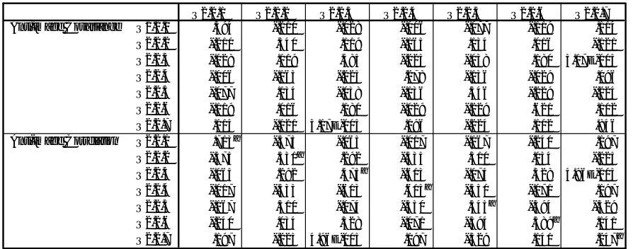
Now, after testing the adequacy of data, the set of 7 statements regarding the coding aspects of simulation software were subjected to factor analysis. Principal Component Analysis (PCA) was used for extraction of factors and the number of factors to be retained was on the basis of Latent Root Criterion (Eigen Value Criterion). An eigen value represents the amount of variance associated with the factor. Thus, only the factors having latent roots or eigen values greater than 1 are considered significant; all the factors with latent roots less than 1 are considered insignificant and are disregarded (Hair, 2003, p.103). Therefore, factors with eigen values more than one should be selected. Table 3 contains the initial eigen values for all the components. Perusal of Table 3 indicates that only threee components have eigen values greater than unity and total variance accounted for by these three factors is 75.300 percent and remaining 24.700 percent was explained by other factors.
Table 3: Total Variance Explained by Initial Eigen Values
Total Variance Explained
2.849 40.693 40.693 2.849 40.693 40.693 2.409 34.415 34.415
1.266 18.089 58.782 1.266 18.089 58.782 1.668 23.833 58.248
1.156 16.518 75.300 1.156 16.518 75.300 1.194 17.052 75.300
.926 13.227 88.528
.352 5.022 93.549
.297 4.240 97.789
.155 2.211 100.000
Component 1
2 3 4 5 6 7
Total % of Variance Cumulative % Total % of Variance Cumulative % Total % of Variance Cumulative %
Initial Eigenvalues Extraction Sums of Squared Loadings Rotation Sums of Squared Loadings
Extraction Method: Principal Component Analysis.
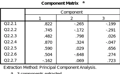
Further, the Component Matrix (without rotation) was constructed as exhibited in Table 4. Perusal of Table 4 indicates that there are many variables having loading on more than one factor. “Although the unrotated factor matrix indicates the relationship between the factors and individual variables, it seldom results in factors that can be interpreted, because factors are correlated with many variables” (Malhotra, 2002, p. 595). The solution to above problem lies in Varimax Rotation.
Table 4: Component Matrix (Without Rotation)
Component Matrix a
.822 -.265 -.199
.745 -.172 -.291
.482 .798 .026
.870 .324 -.047
.590 .029 .656
.504 -.648 .274
-.162 .069 .723
Q2.2.1 Q2.2.2 Q2.2.3 Q2.2.4 Q2.2.5 Q2.2.6 Q2.2.7
1 2 3
Component
Extraction Method: Principal Component Analysis. 3 components extracted.
a.
The factor loadings greater than 0.45 should be retained (ignoring signs) because loadings below it are poor (Bhaduri, 2002, Sidhu and Vasudeva, 2005). The Present study has also followed the same criterion for factor loadings. The Varimax Rotated Factor Loading Matrix has been presented in Table 5.
Table 5: Varimax Rotated Factor Loading Matrix
Rotated Component Matrix a
.862 .194 -.064
.763 .239 -.170
.004 .930 .067
.584 .720 .070
.391 .295 .735
.715 -.316 .371
-.280 -.052 .688
Q2.2.1 Q2.2.2 Q2.2.3 Q2.2.4 Q2.2.5 Q2.2.6 Q2.2.7
1 2 3
Component
Extraction Method: Principal Component Analysis. Rotation Method: Varimax with Kaiser Normalization.
Rotation converged in 6 iterations. a.
Further perusal of Table 5 indicates that variable 2.2.4 had been loaded on two factors namely 1 and 2, but on the basis of higher loading it was considered in Factor 2 only because we know “the process of underlining only the single highest loading as significant for each variable is an ideal” (Hair, 2003, p.113). Ultimately, it was found that the variables 2.2.1, 2.2.2 and 2.2.6 loaded on Factor 1, the variables 2.2.3 and 2.2.4 on Factor 2, 2.2.5 and 2.2.7 on Factor 3.
4.2 Interpretation of Factors:-
A factor loading represents the correlation between variable and its factor. Their signs are just like any other correlation coefficient. Like signs mean the variables are positively related and opposite signs mean the variables are negatively related. In fact the variables carried out in this research study do not reveal any negative related factor loading.
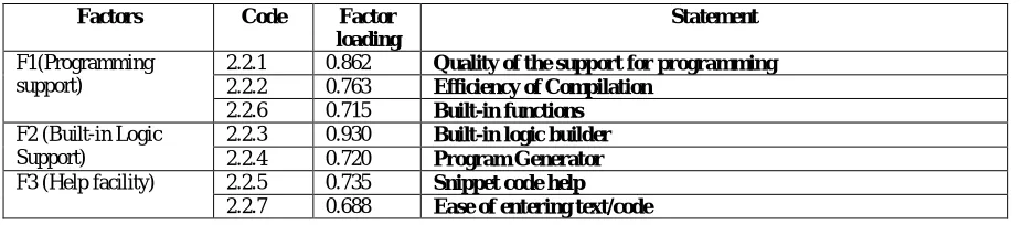
Now, question arises that how to label these factors? Factors can be labeled symbolically as well as descriptively. Symbolic tags are precise and help avoiding confusion (Rummel, 1970). Present study has also given symbolic labels to the factors. The factors along with their codes and factor loadings are given in Table 6.
Table 6: Interpretation of Factors (For Coding Aspects)
Factors Code Factor
loading
Statement
F1(Programming support)
2.2.1 0.862 Quality of the support for programming 2.2.2 0.763 Efficiency of Compilation
2.2.6 0.715 Built-in functions F2 (Built-in Logic
Support)
2.2.3 0.930 Built-in logic builder 2.2.4 0.720 Program Generator F3 (Help facility) 2.2.5 0.735 Snippet code help
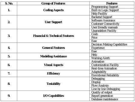
Similarly, the PCA have been applied on other groups of criteria and Factors identified are summarized as shown in Table below:
Table 5.27: Summary of Factors in Different Groups of Features
V. SUMMARY AND CONCLUSIONS
This paper presents the solution methodology for large organizations for the evaluation and selection of simulation software, which are continuously increasing in number. Each vendor claims his product to be the best solution for the organization. Principal Component Analysis have been applied to solve the problem. It gives a very systematic way to select the simulation package satisfying organization’s requirements.
ACKNOWLEDGEMENTS
Much of the information in this paper was derived from extended discussions with software vendor personnel. The authors gratefully acknowledge the time investments in this project that were generously provided by Mr. Jai Shankar from ProModel Corporation, Mr. Kiran Vonna from CD-adapco India Pvt. Ltd. and Mr. Suru from Escorts Group, Mr. Beth Plott from Alion Science and Technology.
S. No. Group of Features Features
1. Coding Aspects
Programming Support Built-in Logic Support Help Facility
2. User Support
Backend Support Software Assurance Customer Connectivity User friendly manuals
3. Financial & Technical Features
Upgradation Facility Costs
Price Ease
4. General Features
Decision Making Capabilities Experience
Ease
5. Modeling Assistance Help
Warning Alerts
6. Visual Aspects
Animation
Customization Facility Real-time Animation
7. Efficiency Adaptability
Executional Reliability
8. Testability
Debugging Display Flow Analysis
Line by line Debugging
9. I/O Capabilities
REFERENCES
1. Abed, S.Y., Barta, T.A. and McRoberts, K.L. 1985a. A Qualitative Comparison of Three Simulation Languages: GPSS/H, SLAM, SIMSCRIPT. Computers and Industrial Engineering, 9: 136-144.
2. Atkins, M.S. 1980. A Comparison of SIMULA and GPSS for Simulating Sparse Traffic. Simulation, 34: 93-98.
3. Banks, J., Aviles, E., McLaughlin, J.R. and Yuan, R.C. 1991. The Simulator: New Member of the Simulation Family. Interfaces, 21 (1): 76-86. 4. Bollino, A. 1988. Study and Realisation of Manufacturing Scheduler using FACTOR. Proceedings of the 4th International Conference on
Simulation in Manufacturing, London. 9-20.
5. Ekere, N. N. and Hannam, R.G. 1989. An Evaluation of Approaches to Modeling and Simulating Manufacturing Systems. International Journal of Production Research, 27 (4): 599-611.
6. Fan, I.S. and Sackett, P.J. 1988. A PROLOG Simulator for Interactive Manufacturing Systems Control. Simulation, 50(6): 239-247. 7. Grant, J.W. and Weiner, S.A. 1986. Factors to Consider in Choosing a Graphical Animated Simulation System. Industrial Engineer, 40: 65-68. 8. Hair, J., Rolph, A., Tatham, R., & Black, W. (2003). Multivariate Data Analysis(4th Ed.). New Jersey: Prentice-Hall Publishers.
9. Hlupic, V. and Paul, R.J. 1999. Guidelines for Selection of Manufacturing Simulation Software. IIE Transactions, 31: 21-29. 10. Law, A.M. and Kelton, W.D. 1991. Simulation Modelling and Analysis,2nd edn, Singapore; McGraw-Hill.
11. Law, A.M. and Haider, S.W. 1989. Selecting Simulation Software for Manufacturing Applications: Practical Guidelines and Software Survey. Industrial Engineer, 34: 33-46.
12. Malhotra, N. K. (2002). Marketing Research (4th Ed.). Singapore: Pearson Education.
13. Scher, J.M. 1978. Structural and Performance Comparison between SIMSCRIPT 11.5 and GPSS V. Proceedings of the 9th Annual Conference on Modeling and Simulation, Pittsburgh, 1267-1272.
14. Sen, M. & Pattanayak, J. K. (2005). An Empirical Study of the Factors Influencing the Capital Structure of Indian Commercial Banks. The ICFAI Journal of Applied Finance, 2(3): 53-67.
15. Taramans, S.R. 1986. An Interactive Graphic Simulation Model for Scheduling the factory of the Future. Proceedings of the AUTOFACT '86 Conference, Detroit. 4-31.