Solving resource-constrained shceuling problems with exact methods

Solving Resource-Constrained

Scheduling Problems with Exact

Methods

Jordi Coll Caballero

Advisor: Enric Rodr´ıguez Carbonell

Department of Computer Science

Co-Advisor: Josep Suy Franch

Departament d’Inform`

atica, Matem`

atica Aplicada i Estad´ıstica

Universitat de Girona

Defense date: 4th of July of 2016

Master in Innovation and Research in Informatics

Advanced Computing

Abstract

Scheduling problems mainly consist in finding an assignment of execution times (a schedule) to a set of activities of a project that optimizes an objective function. There are many constraints imposed over the activities that any schedule must satisfy. The most usual constraints establish precedence relations between activities, or limit the amount of some resources that the activ-ities can consume. There are many scheduling problems in the literature that have been and are currently still being studied. A paradigmatic example is the Resource-Constraint Project Scheduling Problem (RCPSP). It consists in finding a start time for each one of the activities of a project, respecting pre-defined precedence relations between activities and without exceeding the capacity of a set of resources that the activities consume. The goal is to find a schedule with the minimum makespan (total execution time of the project). The RCPSP has many gen-eralizations, one of which is the Multimode Resource-Constrained Project Scheduling Problem (MRCPSP). In this variation, each activity has several available execution modes that differ in the duration of the activity or the demand of resources. A solution for the MRCPSP determines the start times of the activities and also an execution mode for each one. These problems are NP-hard, and are known in the literature to be especially hard, with moderately small instances of 50 activities that are still open.

There are many approaches to solving RCPSP and MRCPSP in the literature. They are often tackled with metaheuristics due to their high complexity, but there are also some exact ap-proaches, including Mixed Integer Linear Programming (MILP), Branch-and-Bound algorithms or Boolean Satisfiability (SAT), which have shown to be competitive and in many cases even better than metaheuristics. One of the exact methods that is growing in use in the field of con-strained optimization is SAT Modulo Theories (SMT). This thesis is the continuation of previous works carried out in the Logic and Programming (L∧P) group of Universitat de Girona, which used SMT to tackle RCPSP and MRCPSP. Excluding these, there have not been any other attempts to use SMT to solve the MRCPSP. SMT solvers (like other generic methods such as SAT or MILP) do not know which is the problem they are dealing with. It is the work of the modeler to provide a representation of the problem (i.e. an encoding) in the language that the solver admits.

The main goal of this thesis is to use SMT to solve the Multimode Resource-Constraint Project Scheduling Problem. We focus on two already existing encodings for the MRCPSP, namely thetime encoding and thetask encoding. We use some existing preprocessing methods that contribute to the formulation of time and task, and present new preprocessings. Most of them are based on the idea of incompatibility between two activities, i.e., the impossibility that two activities run at the same time instant. These incompatibilities let us discharge some con-figurations of the solutions prior to encode the problem. Consequently, the use of preprocessings helps to reduce the size of the encodings in terms of variables and clauses. Another contribution of this work is the study of thetime and task encodings and the differences that they present. We refine these encodings to provide more compact versions. Moreover, two new versions of these encodings are presented, which mainly differ in the codification of the constraints over the use of resources. One of them is based on Linear Integer Arithmetic expressions, and the other one in Pseudo-Boolean constraints and Integer Difference Logic. Another contribution of this work is the presentation of an ad-hoc optimization algorithm based on a linear search that mainly consists in three steps. First of all it simplifies the problem to efficiently ensure or discharge the feasibility of the instance, then it finds a first non-optimal solution by using a quick heuristic method, and finally it optimizes the problem making use of the knowledge acquired with the

preprocessings to boost the search. We also present an initial work on a more intrusive approach consisting in modifying the internal heuristic of the SMT solver for the decision of literals. This work involves the study of a state-of-the-art implementation of an SMT solver, and its modifica-tion to include a framework to specify heuristics related with the encoding of the problem. We give some initial results on custom heuristics for thetime and task encodings of the MRCPSP.

Finally, we test our system with the benchmark sets of instances for the MRCPSP available in the literature, and compare our performance with a state-of-the-art exact solver for the MRCPSP. The results show that we are able to solve the major part of the benchmark sets. Moreover, we show to be competitive with the state-of-the-art solver of V´ılim et. al. for the MRCPSP, being our system slower in solving the easiest benchmark instances, but outperforming the solver of V´ılim et. al. in solving the hardest instances.

Contents

I

Introduction

3

1 Introduction and Motivation 4

II

Antecedents

6

2 Problem Definition 7

2.1 RCPSP . . . 7

2.2 MRCPSP . . . 8

2.3 Benchmark Instances of Scheduling Problems . . . 10

3 Satisfiability Modulo Theories 12 3.1 SAT/SMT Solving . . . 12

3.2 Linear Integer Arithmetic . . . 15

4 State of the Art 16 4.1 Preprocessings . . . 16

4.1.1 Extended Precedence Set . . . 16

4.1.2 Lower Bound . . . 17

4.1.3 Upper Bound . . . 17

4.1.4 Time Windows . . . 17

4.1.5 Non-Renewable Resource Demand Reduction . . . 18

4.2 PSS Heuristic . . . 18

4.3 Encodings . . . 19

4.3.1 Time Formulation . . . 20

4.3.2 Task Formulation . . . 20

4.4 Optimization of the Makespan . . . 21

4.5 Pseudo-Boolean Constraints . . . 23

III

Development and Evaluation of the Proposal

25

6.2 Experimental Settings . . . 27

7 Preprocessings 29

7.1 New Preprocessings . . . 29

7.1.1 Extended Precedence Set: Energy Precedences . . . 29

7.1.2 Start Time Window Incompatibilities . . . 30

7.1.3 Resource Incompatibilities . . . 30

7.1.4 Disjoint Use of Renewable Resources . . . 31

7.2 Impacts of the Preprocessings . . . 31

8 Encoding Study and Refinement 35 8.1 Study of the Encodings . . . 35

8.2 Application of the New Preprocessings . . . 37

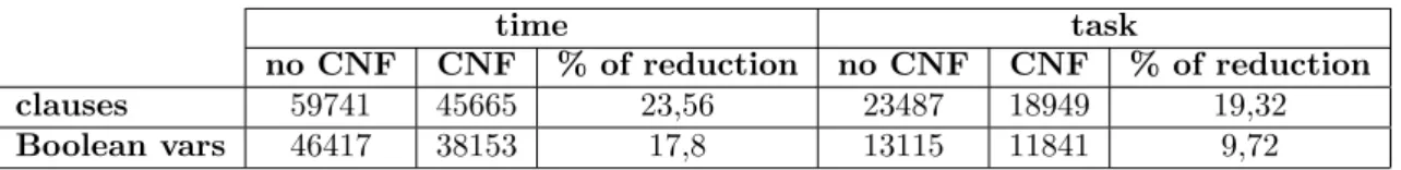
8.3 CNF Conversion . . . 39

8.4 Three Versions of the Encodings . . . 40

8.4.1 Ite: Use of if-then-else Expressions . . . 41

8.4.2 Mult: Use of 0/1 Integer Variables . . . 42

8.4.3 BDD: Pseudo-Boolean Constraints . . . 44

8.5 Results . . . 45

8.5.1 Application of the New Preprocessings . . . 46

8.5.2 CNF Conversion . . . 46

8.5.3 Ite,Mult andBDD . . . 50

9 Optimization Procedure 53 9.1 Detecting Infeasibility . . . 53

9.2 Adjusting the Upper Bound for the Optimum Makespan . . . 54

9.3 Optimizing the Makespan . . . 56

9.3.1 Encoding Size Reduction . . . 58

9.3.2 Mixed Strategies . . . 64

9.3.3 Quantification of the Simplification . . . 68

10 Decision Heuristics 71 10.1 Study of Yices 2 Implementation . . . 71

10.1.1 SMT Core . . . 73

10.1.2 Internalization of the Terms . . . 75

10.2 An Extension to Support User-Defined Heuristics . . . 76

10.2.1 Extension of the API . . . 76

10.2.2 Implementation of the Extension . . . 77

10.3 Heuristics for the MRCPSP . . . 79

10.3.1 Decide Allowed Heuristics . . . 79

10.3.2 Order Heuristics . . . 81

10.4 Results . . . 82

11 Performance of the Techniques 84

Part I

Chapter 1

Introduction and Motivation

Scheduling problems mainly consist in finding an assignment of execution times (a schedule) to a set of activities of a project that optimizes an objective function. There are many constraints imposed over the activities that any schedule must satisfy. The most usual constraints establish precedence relations between activities, or limit the amount of some resources that the activities can consume. Therefore, scheduling problem is a generic term that includes a whole family of problems that fit the former definition. It has been and it is still a hot research topic, existing very diverse recent publications on solving scheduling problems with different approaches as we show in the state of the art in Section 4.

There are many well defined kinds of scheduling problems in the literature that have been and are currently still being studied. A paradigmatic example is the Resource-Constraint Project Scheduling Problem (RCPSP). It consists in finding a start time for each one of the activities of a project, respecting pre-defined precedence relations between activities and without exceeding the capacity of a set of resources that the activities consume. The activities are non-preemptive, what means that once they start they cannot be paused, and will be running all their duration. The resources are renewable, what means that they have a fixed capacity that is occupied in some units for an activity while it is being executed, and these units are released when the activity finishes its execution. Some examples of renewable resources are workers (an activity requires many workers), or memory for a CPU. The goal is to find a schedule with the minimum makespan (total execution time of the project). The RCPSP has many generalizations, one of which is the Multimode Resource-Constrained Project Scheduling Problem (MRCPSP). In this variation, each activity has several available execution modes. Every mode can differ in the duration of the activity and the demand over the resources. A solution for the MRCPSP determines the start times of the activities and also an execution mode for each one. Moreover, there may be non-renewable resources as well as the renewable resources. A non-renewable resource has a capacity that decreases as the activities use it, and cannot be recovered. Hence, it is needed to ensure that the overall use of these resources during the whole project is not bigger than their capacity. A budget or raw material are some examples of non-renewable resources.

These scheduling problems are NP-hard, and are known in the literature to be especially hard. There are instances of problems with projects of 50 or less activities that are still open. For this reason, there are many approaches to solving these problems in the literature. They are often tackled with metaheuristics due to their high complexity, but these approaches do not guarantee the optimality of the solutions that they find. Nevertheless, there are also some exact approaches, which have shown to be competitive and are in many cases even better than metaheuristics. Moreover, in the case of exact methods, the optimality of the solutions is mathematically proven.

Most of them are generic solving methods that offer a language to model constraint satisfaction and optimization problems. We can find approaches in the literature that tackle the RCPSP and the MRCPSP with, among others, Mixed Integer Linear Programming (MILP), branch-and-bound algorithms or Boolean satisfiability (SAT). One of the exact methods that is growing in use in the field of constrained optimization is SAT Modulo Theories (SMT), which is a generalization of SAT (satisfiability of Boolean propositional formulas), which allows to include expressions of a background theory in the formulas. Some of the most common theories are Linear Arithmetic or Uninterpreted Functions.

In this thesis we use SMT to tackle the MRCPSP problem. It has been done in collaboration with the Logic and Programming (L∧P) research group of Universitat de Girona, which have some previous work on solving scheduling problems with SMT ( [3], [37]). Excluding this, and as far as we know, there have not been any other attempts to solve the RCPSP family of problems using SMT. We focus on the study and refinement of two different already existing

SMT formulations of the MRCPSP, namelytime andtask. The contributions of this work can

be summarized as follows:

1. We introduce new preprocessings that let us know some properties of the projects to sched-ule, and simplify the encodings by using this knowledge. By doing it, we are able to sub-stantially reduce the sizes of the encodings, both in number of variables and number of constraints, and also truncating the search space.

2. We provide two new alternative versions of thetask andtimeSMT encodings, one of them based on Linear Integer Arithmetic and the other one in Pseudo-Boolean constraints. 3. We propose algorithms to guide the optimization process by using the knowledge acquired

with the preprocessings.

4. Finally, we explore a more intrusive approach consisting on the modification of the internal solving process of the SMT solver, concretely the heuristic of the decision of variables, to follow a user-defined criterion related with the given encoding.

The remaining of this document is structured as follows. In the second part, II Antecedents, we present all the basic knowledge related with this thesis. In Chapter 2, we state the formal definition of one of the paradigmatic scheduling problems, which is the RCPSP, and we also introduce the problem that we tackle in this thesis, which is the MRCPSP. We also present there the different benchmark sets that are currently being used for the MRCPSP. Chapter 3 contains an insight on Satisfiability Modulo Theories, presenting the basics on modelling language and solving methods. In Chapter 4 we present the state of the art on solving the MRCPSP, with special emphasis on a previous system based on SMT, whose techniques are reused in this thesis. The third part,III Development and evaluation of the proposal, exposes all the new contributions of this thesis and its results. First of all, and having presented the basics on scheduling problems and SMT solving, we expose in Chapter 5 the detailed goals of the thesis. In Chapter 6 we describe the settings of the different experiments contained in this document. In Chapter 7 we present new preprocessings and evaluate the impact that they have in solving different instances. Chapter 8 contains new variations for thetimeandtaskencodings for the MRCPSP. In Chapter 9 we present a generic ad-hoc optimization algorithm, and study how the use of preprocessings can be used to provide information to the SMT solver as we get close to the optimum makespan, and speedup this process. In Chapter 10 we present a framework to provide user-defined heuristics for the decision of variables to the SMT solver, and use it to study the performance oftime and task encodings with several heuristics. Chapter 11 contains the time results of our system on different benchmark sets, and the comparison with the state-of-the-art solver for the MRCPSP. We finally present the conclusions of this thesis in Chapter 12.

Part II

Chapter 2

Problem Definition

2.1

RCPSP

The RCPSP is defined by a tuple (V, p, E, R, B, b) where:

• V = {A0, A1, . . . , An, An+1} is a set of activities. A0 and An+1 are dummy activities representing by convention, thestarting and the finishing activities respectively. The set of non-dummy activities is defined byA={A1, . . . , An}.

• p∈Nn+2_{is a vector of durations. p}

idenotes the duration of activityi, withp0=pn+1= 0 andpi>0,∀i∈ {1, . . . , n}.

• E is a set of pairs representing precedence relations. Thus (Ai, Aj)∈ E means that the

execution of activityAi must precede that of activity Aj, i.e., activityAj must start after

activityAi has finished. We assume that we are given a precedence activity-on-node graph

G= (V, E) that contains no cycles; otherwise the precedence relation is inconsistent. Since precedence is a transitive binary relation, the existence of a path in Gfrom the nodei to node j means that activity i must precede activityj. We assume thatE is such thatA0 is a predecessor of all other activities andAn+1 is a successor of all other activities.

• R={R1, . . . , Rm} is a set ofm renewable resources.

• B ∈ Nm _{is a vector of resource availabilities. B}

k denotes the available amount of each

resource Rk.

• b∈N(n+2)×m _{is a matrix ofdemands of activities for resources. The valueb}

i,k represents

the amount of resourceRkused during the execution ofAi. Note thatb0,k= 0,bn+1,k= 0

andbi,k≥0,∀i∈ {1, . . . , n},∀k∈ {1, . . . , m}.

A schedule is a vector S = (S0, S1, . . . , Sn, Sn+1) where Si denotes the start time of each

activityAi∈V. We assume thatS0= 0. A solution to an RCPSP instance is a non-preemptive (an activity cannot be interrupted once it is started) schedule S of minimal makespan Sn+1 subject to the precedence and resource constraints:

subject to:

Sj−Si≥pi ∀(Ai, Aj)∈E (2.2)

∑

Ai∈At

bi,k≤Bk ∀Bk ∈B,∀t∈H (2.3)

where At={Ai ∈A |Si ≤t < Si+pi} represents the set of non-dummy activities in process

at timet, the setH ={0, . . . , T}is the scheduling horizon, andT (the length of the scheduling horizon) is an upper bound for the makespan. A scheduleSis feasible if it satisfies the generalized precedence constraints (2.2) and the resource constraints (2.3).

2.2

MRCPSP

The MRCPSP is a generalization of the RCPSP. It is defined by a tuple (V, M, p, E, R, B, b) where :

• V = {A0, A1, . . . , An, An+1} is a set of activities. Activities A0 and An+1 are dummy activities representing, by convention, the start and the end of the schedule, respectively. The set of non-dummy activities is defined byA={A1, . . . , An}.

• M ∈ Nn+2 is a vector of naturals, being Mi the number of modes that activity i can

execute, withM0=Mn+1= 1 andMi≥1,∀Ai ∈A.

• pis a vector of vectors of naturals, beingpi,otheduration of activityiusing modeo, with

1 ≤o≤Mi. For the dummy activities,p0,1 =pn+1,1= 0, and pi,o >0,∀Ai∈A,1≤o≤

Mi .

• E is a set of pairs of activities representing precedence relations. Concretely, (Ai, Aj)∈E

iff the execution of activityAi must precede that of activityAj, i.e., activityAj must start

after activityAi has finished.

We assume that we are given a precedence activity-on-node graphG= (V, E) that contains no cycles, since otherwise the precedence relation is inconsistent. We assume thatEis such thatA0is a predecessor of all other activities andAn+1is a successor of all other activities.

• R ={R1, . . . , Rv−1, Rv, Rv+1, . . . , Rq} is a set of resources. The first v resources are

re-newable, and the lastq−v resources are non-renewable.

• B ∈ Nq is a vector of naturals, being Bk the available amount of each resource Rk. The

first v resource availabilities correspond to the renewable resources, while the last q−v ones correspond to the non-renewable resources.

• b is a matrix of naturals corresponding to the resource demands of activities per mode. The valuebi,k,orepresents the amount of resourceRk used during the execution of activity

Aiin modeo. Note that b0,k,1= 0 andbn+1,k,1= 0,∀k∈ {1, . . . , q}.

A schedule is a vector of naturals S = (S0, S1, . . . , Sn, Sn+1) where Si denotes the start

time of activity Ai. We assume that S0 = 0. A schedule of modes is a vector of naturals SM= (SM0,SM1, . . . ,SMn,SMn+1) whereSMi, satisfying 1≤SMi≤Mi, denotes the mode of

each activityAi. A solution to an MRCPSP instance is aschedule of modesSMand a schedule

S of minimal makespanSn+1. The MRCPSP can hence be formulated as

subject to the following precedence and resource constraints: (SMi=o)→(Sj−Si≥pi,o) ∀(Ai, Aj)∈E,∀o∈ {1, . . . , Mi} (2.5)  ∑ Ai∈A ∑ o_∈{1,...,M_i} ite(SMi=o;bi,k,o; 0)  _≤Bk ∀Rk ∈ {Rv+1, . . . , Rq} (2.6)  ∑ Ai∈A ∑ o∈{1,...,Mi}

ite((SMi=o)∧(Si≤t)∧(t < Si+pi,o);bi,k,o; 0)

 _≤Bk

∀Rk∈ {R1, . . . , Rv},∀t∈H

(2.7)

where ite(c;e1;e2) is an if-then-else expression denoting e1 ifc is true and e2 otherwise, H =

{0, . . . , T} is the scheduling horizon, and T (the length of the scheduling horizon) is an upper bound for the makespan.

We also have to force the execution mode to be correct:

SMi≥1 ∀Ai∈A (2.8)

SMi≤Mi ∀Ai∈A (2.9)

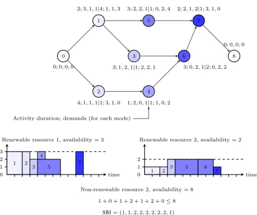
A schedule S is feasible if it satisfies the precedence constraints (2.5), the non-renewable resource constraints (2.6), the renewable resource constraints (2.7) and the execution mode cor-rectness constraints (2.8) and (2.9). Figure 2.1 shows an example of an MRCPSP instance and solution that we will use as a running example to introduce some concepts.

Hence, the main differences with respect to the RCPSP are that MRCPSP include non-renewable resources, and that each activity has several execution modes.

An MRCPSP instance has a feasible schedule if and only if the following conditions hold:

• There not exist a cycle in the precedence graph (i.e., an activity is forced to start after itself finishes).

• There not exist any activity whose demand over a resource in all execution modes is greater than its capacity.

• There exist a schedule of modes such that all the non-renewable resource constraints (2.6) are satisfied.

The first two conditions are typically satisfied in the different benchmark set of instances available in the literature because they can be easily verified and therefore instances with these sources of infeasibility are not worth to study. This is not the case for the third condition, which introduces a combinatorial component to the problem. For this reason, in contrast with the RCPSP, there are benchmark sets for the MRCPSP containing infeasible instances; see Section 2.3 for more details.

0 0; 0,0,0 1 2; 3,1,1|4; 1,1,3 2 4; 1,1,1|1; 3,1,0 3 3; 1,2,1_|1; 2,2,1 4 1; 2,0,1|1; 1,0,2 5 3; 2,2,1|1; 0,2,4 6 3; 0,2,1|2; 0,2,2 7 2; 2,1,2|1; 3,1,0 8 0; 0,0,0

Activity duration; demands (for each mode)

1 2 3 4 5 7 3 2 1 0 time

Renewable resource 1, availability = 3

1 2 3 5 6 7

2 1

0 time

Renewable resource 2, availability = 2

Non-renewable resource 2, availability = 8 1 + 0 + 1 + 2 + 1 + 2 + 0≤8

SM= (1,1,2,2,2,2,2,2,1)

Figure 2.1: An MRCPSP instance of 7 non-dummy activities, two renewable resources and one non-renewable resource. The graph represents the activity precedences. Each node is an activity, and the numbers near the node express, for each execution mode (separated by |), its duration and the demand of the resources. Under the graph there is represented a solution, where the Gantt diagrams show the use of the renewable resources at all times, as well as the execution times of the activities.

2.3

Benchmark Instances of Scheduling Problems

Most of the works on MRCPSP in the literature [41, 40, 10] evaluate the performance of their systems using the instances available of PSPLib [25]. PSPLib is a library of benchmark sets of instances for scheduling problems which contains, among others, sets for the RCPSP and the

MRCPSP. The datasets are publicly available at its web sitewww.om-db.wi.tum.de/psplib/.

Regarding the MRCPSP, it contains the sets of instances described in Table 2.1.

The set j30 set will be used as a training set in this thesis, because it contains variety of instances in what regards to their hardness (it has many soft instances and at the same time is the only one in PSPLib with open instances), and also contains both feasible and infeasible instances. Will treat feasible and infeasible instances independently in many cases. From now on, we will refer toj30SAT as the subset of j30 that contains all the feasible instances, and to j30UNSAT as the subset containing all the infeasible instances. j30SAT contains 552 instances, and j30UNSAT contains 88 instances.

There is also MMLIB [39], a more recent repository of benchmark datasets for scheduling

problems, including MRCPSP. They are publicly available athttp://www.projectmanagement.

set instances activities modes renewable res. non-ren. res. j10 537 10 3 2 2 j12 547 12 3 2 2 j14 551 14 3 2 2 j16 550 16 3 2 2 j18 552 18 3 2 2 j20 554 20 3 2 2 j30 640 30 3 2 2 m1 640 16 1 2 2 m2 481 16 2 2 2 m4 555 16 4 2 2 m5 558 16 5 2 2 r1 553 16 3 1 2 r3 552 16 3 3 2 r4 557 16 3 4 2 r5 546 16 3 5 2 n0 470 [10-20] 3 2 0 n1 637 16 3 2 1 n3 600 16 3 2 3 c15 551 16 3 2 2 c21 552 16 3 2 2

Table 2.1: Benchmark sets of PSPLib

MMLIB50 540 instances with 50 activities, each one with 3 execution modes. There are 2 renewable resources and 2 non-renewable resources.

MMLIB100 540 instances with 100 activities, each one with 3 execution modes. There are 2 renewable resources and 2 non-renewable resources.

MMLIB+ 3240 instances with 50 or 100 activities, each one with 3, 6 or 9 execution modes. The number of renewable and non-renewable resources are 2 or 4.

These instances are harder than the ones in PSPLib, and they are more recent. There are still not many works that solve them, but we can find some that use non-exact methods [20, 11].

Chapter 3

Satisfiability Modulo Theories

Satisfiability Modulo Theories (SMT) is a generalization of Boolean satisfiability. An SMT formula is a Boolean formula in which, in addition to Boolean variables, there can also occur predicates with predefined interpretations from background theories. The following is an example of SMT formula that includes the theory of Linear Integer Arithmetic:

(p∨q)∧(¬p∨x≤y)∧(x >3∨y >3)

where pand qare Boolean variables, andx andy are integer variables. The following is some basic nomenclature of SMT formulas:

• An atom is a predicate of the theory. In the previous formula, there appear the atoms x≤3,x >3 andy >3.

• Aliteral is an occurrence of a Boolean variable or an atom in a formula, or an occurrence of their negation. In our example,p,q,¬p,x≤3,x >3 andy >3 are literals.

• A formula is in Conjunctive Normal Form (CNF) if it is a conjunction of clauses, which are disjunctions of literals. The previous formula is in CNF, and its clauses are (p∨q), (¬p∨x≤y) and (x >3∨y >3).

The most common theories of the predicates appearing in SMT formulas are linear real or integer arithmetic, arrays, bit vectors, uninterpreted functions, or combinations of them. The expressibility of this language makes SMT a very good approach to model Constraint Satisfaction Problems. SMT is a good option as well taking into account efficiency, since current SMT solvers

have shown to be very competitive with other model-and-solve exact approaches such as SAT

or MILP. In Section 3.1 we make an overview on the basics on SAT / SMT solvers, and we introduce in Section 3.2 the theories of Linear Integer Arithmetic and Difference Logic, which are going to be used in this thesis.

3.1

SAT/SMT Solving

Current SMT solvers are based on the DPLL [13, 12] procedure for SAT solving. It is a procedure that can be modelled by a transition relation over states [29]. A state is either FailState or a

pair M ∥ ϕ, where ϕ is a finite set of clauses and M is a partial assignment (in the form of a

the ones added to M by theDecide rule, and are writtenld_{. The transition relation is defined}

by means of rules.

The classical DPLL transition system consists of the following five rules: UnitPropagate : M ∥ϕ, C∨l =⇒ M l∥ϕ, C∨l if { M |=¬C and lis undefined inM. PureLiteral : M ∥ϕ =⇒ M l∥ϕ if     

l occurs in some clause ofϕ,

¬l occurs in no clause ofϕand l is undefined inM.

Dedide :

M ∥ϕ =⇒ M ld∥ϕ if

{

lor ¬loccurs in some clause of ϕand lis undefined inM.

Fail :

M ∥ϕ, C =⇒ FailState if

{

M |=¬C and

M contains no decision literals. Backtrack :

M ld_{N ∥ϕ, C =⇒ M¬l∥ϕ, C if}

{

M ldN|=¬Cand

N contains no decision literals.

The PureLiteral rule is usually used as a preprocessing step. Then, the evolution of the transition system follows these basic steps:

1. ApplyUnitPropagate while possible.

2. IfM contains all the variables, it is a complete assignment (ormodel) of the formula, i.e. a solution, and the procedure halts.

3. If we can applyF ail, the formula is unsatisfiable, and the procedure halts.

4. If we can apply Backtrack, we have found a conflict. We apply the Backtrack rule and return to step 1.

5. We apply theDecide rule, and return to step 1.

Most of modern DPLL algorithms replace the Backtrack rule by the Backjump rule and add

three new rules:

• the Learn rule which implements the so-called Conflict-Driven Clause-Learning (CDCL). After a conflict is encountered, an explanation for it (a lemma) is learnt, in the form of a new clause.

• theForget rule that is used to forget learned clauses (usually for reasons of space)

Backjump : M ldN ∥ϕ, C =⇒ M l′∥ϕ, C if                M ld_{N |=¬C and there is}

some clauseC′∨l′ such that: ϕ, C|=C′∨l′ andM |=¬C′, l′ is undefined inM, and l′ or¬l′ occurs inϕor inM ld_N. Learn : M ∥ϕ =⇒ M ∥ϕ, C if {

all atoms ofCoccur inϕor inM and ϕ|=C.

Forget:

M ∥ϕ, C =⇒ M ∥ϕ if ϕ|=C.

Restart :

M ∥ϕ =⇒ ∅ ∥ϕ.

Solvers using CDCL are often referred to as CDCL solvers. The following is an example of application of the DPLL rules on the formula (¬x1∨x2)∧(¬x3∨x4)∧(¬x5∨¬x6)∧(x6∨¬x5∨¬x2), were we underline the clause causing theBackjump orUnitPropagation:

∅ ∥ ¬x1∨x2,¬x3∨x4,¬x5∨ ¬x6, x6∨ ¬x5∨ ¬x2 ⇒ Decide xd 1 ∥ ¬x1∨x2,¬x3∨x4,¬x5∨ ¬x6, x6∨ ¬x5∨ ¬x2 ⇒ UnitPropagate xd 1x2 ∥ ¬x1∨x2,¬x3∨x4,¬x5∨ ¬x6, x6∨ ¬x5∨ ¬x2 ⇒ Decide xd 1x2xd3 ∥ ¬x1∨x2,¬x3∨x4,¬x5∨ ¬x6, x6∨ ¬x5∨ ¬x2 ⇒ UnitPropagate xd 1x2xd3 x4 ∥ ¬x1∨x2,¬x3∨x4,¬x5∨ ¬x6, x6∨ ¬x5∨ ¬x2 ⇒ Decide xd 1x2xd3 x4x5d ∥ ¬x1∨x2,¬x3∨x4,¬x5∨ ¬x6,x6∨ ¬x5∨ ¬x2 ⇒ UnitPropagate xd

1x2xd3 x4xd5¬x6 ∥ ¬x1∨x2,¬x3∨x4,¬x5∨ ¬x6,x6∨ ¬x5∨ ¬x2 ⇒ Backjump&Learn xd₁x2¬x5 ∥ ¬x1∨x2,¬x3∨x4,¬x5∨ ¬x6, x6∨ ¬x5∨ ¬x2,¬x2∨ ¬x5 ⇒ Decide xd 1x2¬x5xd3 ∥ ¬x1∨x2,¬x3∨x4,¬x5∨ ¬x6, x6∨ ¬x5∨ ¬x2,¬x2∨ ¬x5 ⇒ UnitPropagate xd₁x2¬x5xd₃x4 ∥ ¬x1∨x2,¬x3∨x4,¬x5∨ ¬x6, x6∨ ¬x5∨ ¬x2,¬x2∨ ¬x5 ⇒ Decide xd 1x2¬x5xd3x4¬xd6 ∥ ¬x1∨x2,¬x3∨x4,¬x5∨ ¬x6, x6∨ ¬x5∨ ¬x2,¬x2∨ ¬x5 ⇒ SOLUTION

In [29], we can find an adaptation to SMT of the DPLL procedure, called DPLL(T), where T stands for the parametrization on a theory. Similarly, SMT solvers using CDCL are referred to as CDCL(T) solvers.

We will not enter in detail into CDCL(T), but basically it follows the following mechanism. There is a previous step that converts an SMT formula to a SAT formula, introducing new Boolean variables in substitution of the atoms. For instance, the SMT formula:

(p∨q)∧(¬p∨x≤y)∧(x >3∨y >3) would be substituted by the Boolean formula:

(p∨q)∧(¬p∨b1)∧(b2∨b3)

whereb1, b2 andb3 are fresh Boolean variables. Then, a mapping is constructed relating atoms and their corresponding Boolean variables:

b2↔x >3 b3↔y >3

In order to solve this system, a modified version of the DPLL procedure is applied to solve the Boolean formula, while interacting with aT-solver (theory solver), which is a module that handles the theory expressions, and is able to check the consistency of Boolean assignments with respect to the theory, detect conflicts, and produce corresponding explanations. We refer the reader to [29] for further details of the CDCL(T) procedure.

The Decide rule is flexible in the sense that it does not require any particular literal to be decided, the only condition is that it is not in the partial assignment. State-of-the-art SAT / SMT solvers use the Variable State Independent Decay (VSID) heuristic to choose the literal to decide [28]), which was engineered for conflict driven solvers. In Chapter 10 we enter in more detail in the decision of literals, and study the behaviour of alternative heuristics for the MRCPSP.

3.2

Linear Integer Arithmetic

The theory of Linear Integer Arithmetic (LIA) includes expressions of the form: a1·x1+· · ·+an·xn#b

where x1, . . . , xn are integer variables, a1, . . . , an are their coefficients, b is a constant term,

and # ∈ {<,≤,=, >,≥}. The interpretations of these expressions follow the arithmetic rules. This theory suits very well to our problem, as we can see in the time and task formulations of Section 4.3. Current theory solvers handling this theory are based on the Simplex method, concretely on the solver introduced in [19].

There is a specialization of LIA called Difference Logic (DL). In DL, the expressions are restricted to have the form:

x−y≤c

where x and y are variables (integer variables in Integer DL), and c is a constant. Most of SMT solvers offer specific theory solvers for DL, based on the Bellman-Ford algorithm or the Floyd-Warshall algorithm, which are often more efficient than the Simplex method of general LIA theory solvers.

Chapter 4

State of the Art

The RCPSP and its variants have been widely studied in the literature. An insight to the prob-lems, their characteristics, and different solving methods can be found in [4]. These problems are usually tackled with meta-heuristics due to their hardness. For the MRCPSP, many approaches have been proposed, including simulated annealing [8, 36], genetic algorithms [21, 2, 42], biased random sampling approaches [16], or neighbourhood search [20]. Nevertheless, exact approaches have shown to be also competitive for scheduling problems. There are many works for the RCPSP based on Constraint Programming (CP) [27, 6], Boolean satisfiability(SAT) [22], Satisfiability Modulo Theories (SMT) [3], Mixed Integer Linear Programming [26], branch and bound algo-rithms [15] and Lazy Clause Generation [33, 32]. Also there have been recent exact approaches to solve the MRCPSP, based on MILP [10], SMT [37], and branch an bound [40]. The lat-ter has shown to be the state-of-the art in exact solving for the MRCPSP, by implementing a conflict-driven branching heuristic that resembles the one used by SAT/SMT solvers.

In this thesis we specially revisit, reuse and extend some of the work that has been published in [37, 7]. The following sections in this chapter expose the already existing techniques in the literature which this thesis builds upon. Section 4.1 contains a set of preprocessing techniques for the MRCPSP. Section 4.2 introduces a heuristic quick method to find initial solutions that is going to be used to set an upper bound of the makespan. Section 4.3 exposes the mentioned timeandtask encodings for this problem. Section 4.5 briefly describes what are Pseudo-Boolean constraints and BDDs, which are going to be used in this thesis.

4.1

Preprocessings

There are some classical preprocessing steps that are used by most of the solvers for scheduling problems. A good insight on these techniques can be found in [4]. We introduce the ones that we are going to use in Sections 4.1.1, 4.1.2, 4.1.3 and 4.1.4. In Section 4.1.5 we explain a new preprocessing technique that was firstly introduced in [37].

4.1.1

Extended Precedence Set

Since a precedence is a transitive relation, we can compute a lower bound on the time between each pair of activities in E. For this calculation it can be used the Floyd-Warshall algorithm on the graph defined by the precedence relationE, where each arc (Ai, Aj) is labelled with the

duration mino_∈{1,...,M_i}(pi,o). This extended precedence set is namedE∗ and contains, for each

is the length of the longest path fromAi to Aj. Note that this longest path length is minimal

with respect to the different activity modes. Note also that, if (Ai, Ai, li,i)∈E∗for someAiand

li,i >0, then there is a cycle in the precedence relation and therefore the problem instance is

inconsistent.

4.1.2

Lower Bound

A lower boundLB for the makespan is a lower bound for the start time of activityAn+1. The critical path (i.e. the maximum length path) between the initial activityA0and the final activity An+1 in the graph gives such a lower bound. Note that we can easily know the length of this path if we have already computed the extended precedence set, since it corresponds to the value l0,n+1 in the tuple (A0, An+1, l0,n+1)∈E∗.

For instance, in the example of Figure 2.1 the critical path is [A0, A1, A3, A6, A7, A8] with modes 1,1,2,2,2,1, respectively, and its length is 6. Hence, we haveLB= 6.

4.1.3

Upper Bound

An upper bound UB for the makespan is an upper bound for the start time of activity An+1. There is atrivial upper bound equal to the sum of the maximum duration of all activities:

UB = ∑

Ai∈A

max

o_∈{1,...,M_i}(pi,o)

In the example of Figure 2.1 this upper bound is 20.

4.1.4

Time Windows

We can reduce the domain of each variable Si (start time of activity Ai), which initially is

{0..UB−mino∈{1,...,Mi}(pi,o)}, by computing itstime window. The time window of activityAi

will be [ESi, LSi], beingESi its earliest start time and LSi itslatest start time. To compute

the time window we use the lower and upper bound and the extended precedence set, as follows. For activitiesAi,0≤i≤n,

ESi=l0,i if (A0, Ai, l0,i)∈E∗

LSi=UB−li,n+1 if (Ai, An+1, li,n+1)∈E∗

and, for activityAn+1,

ESn+1=LB LSn+1=UB

Notice that the size of the time windows depends on a givenUB. For instance, in the example of Figure 2.1, activityA4 has time window [1,16] with the trivialUB = 20.

Based on the time window, we can define for an activity Ai itsearliest completion time and

its latest completion time, which consider the minimum and maximum durations respectively among the different execution modes:

ECi=ESi+ min 1_≤o_≤Mi pi,o ∀Ai∈V LCi=LSi+ max 1≤o≤Mi pi,o ∀Ai∈V

4.1.5

Non-Renewable Resource Demand Reduction

This preprocessing step consists in reducing the demand of non-renewable resources in a sound way. As we will see, this will allow us to save SMT literals in the constraints related to those kind of resources.

Let us introduce it through an example. In the example of Figure 2.1, the non-renewable resource R3 has 8 units available and activity A6 has two modes: mode 1 requires 1 unit of resourceR3, while mode 2 requires 2 units of the same resource. This problem can be transformed into an equivalent one, where the availability of resourceR3 is 7, and activityA6has a demand

of 0 units of resource R3 in mode 1, and of 1 unit in mode 2. Since in mode 1 the demand

is of 0 units, it is not necessary to add any literal considering this mode in the constraints on non-renewable resources. Roughly, following the example, what could be done is to subtract from the availability of resourceR3, and from the different demands of activityA6 for resource R3 in each mode, the minimum amount of resource R3 that activity A6 needs. However, one could go one step further and, instead of subtracting the minimum demand value, subtract the demand value which most frequently occurs. This of course will lead to negative availabilities and demands. But, interestingly, this allows reducing the size of the constraints even more (since more demands become zero), while keeping soundness. Details are given below.

For this preprocessing, we construct a new vector B′ of resource availabilities and a new matrixb′ of resource demands, where:

• B′_k=Bk andb′i,k,o=bi,k,o,∀k∈ {1, . . . , v},∀Ai∈V,∀o∈ {1, . . . , Mi}.

• For each non-renewable resourceRk and activityAi, letmaxk,i denote the demand value

for resourceRk with more occurrences in the different modes of activityAi (and, in case

of a tie, the smallest one). Then we state:

b′_i,k,o=bi,k,o−maxk,i ∀Ai∈A,∀o∈ {1, . . . , Mi}

B_k′ =Bk−

∑

A_i∈A

maxk,i ∀Rk ∈ {Rv+1, . . . , Rq}

Note that, as said, vectorB′ and matrixb′ range now over integers instead of over naturals, i.e., they can contain some negative values. The zero b′_i,k,o values (whose number is maximal thanks to the fact that we subtract the demand value with most occurrences) allow us to simplify the constraints on non-renewable constraints (see Equation 4.10 below).

4.2

PSS Heuristic

In [3], the authors proposed to use a fast heuristic method to find a schedule for the RCPSP, whose makespan serve as an upper bound for the optimum makespan. This upper bound will be in most of the cases better than the trivial upper bound. This heuristic is theparallel scheduling generation scheme (PSS) proposed in [23] and described in [24].

Given a project of n activities, this method requires at most n stages to find an schedule, and at each stage a subset of the activities are scheduled. Each stageshas associated a schedule timets (wherets′ ≤ts, fors′ ≤s). There are three activity sets:

• Complete setC: activities already scheduled and completed up to the schedule timets.

• Decision set D: activities not yet scheduled which are available for scheduling with start timets, w.r.t. precedence and resource constraints.

Each stage consists of two steps:

• Determining the newts: the earliest completion time of activities in the active setA. The

activities with a finish time equal to the new tsare removed fromAand put intoC. This

may place new activities intoD.

• One activity from D is selected with a priority rule (in [3] the activity with the smallest number) and scheduled to start atts, being removed from D and added to A. Then the

set Dis recomputed. This step is repeated until D becomes empty. The method terminates when all activities are scheduled.

This procedure is not suitable for the MRCPSP, since it does not deal with the selection of execution modes, neither with constraints over non-renewable resources. However it has the advantage of being very fast, and serves very well to the purpose of finding a first upper bound. In Section 9.2 we will see how this method can be used for this purpose in the MRCPSP.

4.3

Encodings

In [3], two different SMT encodings for the RCPSP were presented, namely the time encoding

and thetask encoding. They are similar to thetimeformulation of [31] and [26] and to thetask formulation of [30] and [32], but conveniently adapted to SMT.

In [37] the time and task encodings were adapted to the MRCPSP. The authors use the

theory of Linear Integer Arithmetic, which allow to easily encode MRCPSP instances as logical

combinations of arithmetic constraints. With SMT, Boolean variables and integer variables

can occur together in the resulting formula, which is very interesting in terms of modeling. Some refinements were introduced considering the preprocessing steps described in Section 4.1 (extended precedences, time windows, etc.)

The set of integer variables{S0, S1, . . . , Sn, Sn+1}denote the start time of each activity, and S′ is defined as the set{S1, . . . , Sn}. The schedule of modes with the set of Boolean variables

{smi,o |0 ≤i≤n+ 1,1 ≤o ≤Mi}, being smi,o true if and only if activity Ai is executed in

modeo.

The objective function is always (2.4), and there are the following constraints in both encod-ings: S0= 0 (4.1) Si≥ESi ∀Ai∈{A1, . . . , An+1} (4.2) Si≤LSi ∀Ai∈{A1, . . . , An+1} (4.3) smi,o→Sj−Si≥pi,o ∀(Ai, Aj)∈E,∀o∈ {1, . . . , Mi} (4.4) Sj−Si≥li,j ∀(Ai, Aj, li,j)∈E∗ (4.5) sm0,1=true (4.6) smn+1,1=true (4.7) ∨ 1≤o≤Mi smi,o ∀Ai∈A (4.8) ¬smi,o∨ ¬smi,o′ ∀Ai∈A,1≤o≤Mi, o < o′≤Mi (4.9)

where (4.2) and (4.3) encode the time windows, (4.4) encodes the precedences, (4.5) encodes the extended precedences and (4.6), (4.7), (4.8) and (4.9) ensure that each activity runs in exactly one mode.

For non-renewable resources, the following constraints replace (2.6), which use the values resulting from thenon-renewable resource demand reductionpreprocessing step:

       ∑ A_i∈A ∑ o∈ {1, . . . , Mi} b′_i,k,o̸= 0

ite(smi,o;b′i,k,o; 0

)        ≤B_k′ ∀Rk ∈ {Rv+1, . . . , Rq} (4.10)

Notice that theite expression is removed in the cases where b′_i,k,o= 0.

Constraints (2.7) on renewable resources are reformulated differently in each of the two en-codings, as described below.

4.3.1

Time Formulation

This is the most obvious formulation. It basically consists in stating, for every time unitt and renewable resource Rk, that the sum of demands for this resource from the different activities

cannot exceed the availability of the resource.

smi,o→(yi,t↔(Si≤t)∧(t < Si+pi,o))

∀Ai∈A,∀o∈ {1, . . . , Mi},∀t∈ {ESi, . . . , LSi+pi,o} (4.11) ( ∑ A_i∈A ∑ o∈ {1, . . . , Mi} ESi≤t≤LSi+pi,o−1 b′_i,k,o̸= 0

ite(smi,o∧yi,t;b′i,k,o; 0

))

≤B_k′

∀Rk ∈ {R1, . . . , Rv},∀t∈ {0, . . . , U B} (4.12)

Constraints (4.11) give value to the Boolean variables yi,t, which are true if and only if

activity Ai is running at time t. Constraints (4.12) replace the (2.7) of the problem definition.

The number of theses constraints is proportional toU B+ 1, and the size of the sums is directly related to the size of the time windows (which are also dependent onU B). Therefore, the size of this encoding is highly dependent on the value ofU B.

4.3.2

Task Formulation

This formulation uses variables indexed by activity number, and not by time. The key idea is that, in the non-preemptive case, checking only that there is no overload at the beginning (or end) of each activity is sufficient to ensure that there is no overload at every time unit. Hence, in this formulation the number of variables and constraints is independent of the length of the scheduling horizon.

Boolean variablesz1

i,jdenote whether activityAidoes not start after activityAjdoes, Boolean

variablesz2

z1

i,j∧z2i,j denotes whether activity Ai is running when activityAj starts. The constraints are

the following:

z_i,j1 ↔true ∀(Ai, Aj, li,j)∈E∗ (4.13)

z1_j,i↔f alse ∀(Ai, Aj, li,j)∈E∗ (4.14)

zi,j1 ↔Si≤Sj ∀Ai, Aj ∈A, i̸=j (4.15)

z_i,j2 ↔f alse ∀(Ai, Aj, li,j)∈E∗ (4.16)

z_j,i2 ↔true ∀(Ai, Aj, li,j)∈E∗ (4.17)

smi,o→(zi,j2 ↔Sj < Si+pi,o) ∀Ai, Aj∈A,

i̸=j,∀o∈ {1, . . . , Mi} (4.18) smj,o′ →        ∑ A_i∈A_\{Aj} ∑ o∈ {1, . . . , Mi} b′_i,k,o̸= 0

ite(smi,o∧zi,j1 ∧z

2 i,j;b′i,k,o; 0)       ≤ Bk′ −b′j,k,o′ ∀Aj ∈A,∀o′ ∈ {1, . . . , Mj},∀Rk∈ {R1, . . . , Rv} (4.19)

The last constraints (4.19) state, for each activity Aj, mode o′ and renewable resource Rk,

that the sum of resource demands forRk at the start time of Aj must not exceed the capacity

B_k′ ofRk.

4.4

Optimization of the Makespan

SMT has its roots in the field of hardware and software verification, typically dealing with decision problems. For this reason, in the early uses of SMT in the field of constrained problems optimization, many ad-hoc procedures were defined to deal with optimization. One of the basic approaches consists in successively bounding the value of the objective function, until the lower bound coincides with the lower bound and therefore the optimum is found. Nowadays, there are many SMT solvers that support optimization, as is the case of Z3 [14] orOptiMathSAT [35]. The usual behaviour is to combine the computation of Boolean satisfiable models with the optimization of the theory expressions.

Nevertheless, one of the purposes of this thesis is to study the relation of the encoding sizes and computation times as U B evolves. For this reason we will focus on ad-hoc optimization procedures which make independent satisfiability checks to the SMT solver and that let us guide the search of the optimum makespan. Concretely, we will use a linear search optimization scheme (see Algorithm 1), which starts from a feasible U B for the makespan (if any), and reduces it until the instance becomes infeasible.

Algorithm 1Linear search optimization schema

Input: An MRCPSP instanceIN S

Output: Optimum makespan, or INFEASIBLE

UB←get upper bound(IN S)

LB←get upper bound(IN S)

smt assert encoding(EN C)

SAT ←smt check()

if notSAT then

return INFEASIBLE

end if

UB←UB−1

whileSAT and UB≥LB do

smt update upper bound(UB)

SAT ←smt check()

if SAT then

M ODEL←smt get model()

M AKESP AN←smt get makespan(M ODEL)

UB←M AKESP AN−1 end if end while if SAT then return UB else return UB+ 1 end if

x1 x2 x3 x3 x2 x3 x3 0 1 0 1 0 1 0 1 0 1 0 1 0 1 0 1 2x1+ 3x2+ 4x3≤7 3x2+ 4x3≤7 3x2+ 4x3≤5 4x3≤7 4x3≤4 4x3≤5 4x3≤2 Figure 4.1: BDD for 2x1+ 3x2+ 4x3≤7.

4.5

Pseudo-Boolean Constraints

As defined in [1], a Pseudo-Boolean constraint has the form: a1x1+· · ·+anxn#K

where theaiandKare integer coefficients, thexiare Boolean variables, and the relation operator

# belongs to{<, >,≤,≥,=}. A typical data structure to represent Boolean functions is a Binary Decision Diagrams (BDD) [9]. A BDD is a rooted, directed, acyclic graph, where each non-terminal (decision) node corresponds to a Boolean variablexand has two child nodes with edges representing a true and a false assignment to x. There are two terminal nodes that are the 0-terminal and the 1-terminal, representing the truth value of the formula for the assignment leading to them. A BDD is calledordered if the variables appear in the same order on all paths from the root. A BDD is said to bereduced if the following two rules have been applied to its graph until a fix point:

• Merge any isomorphic subgraphs

• Eliminate any node whose two children are isomorphic.

AReduced Ordered Decision Diagram (ROBDD) is canonical (unique) for a particular function and variable order. As an example, we have in Figure 4.1 a BDD that represents the Pseudo-Boolean constraint 2x1+ 3x2+ 4x3≤7, and Figure 4.2 illustrates the canonical ROBDD for the same constraint with the orderx1≺x2≺x3.

In [7], the L∧P group implemented a framework based on the ideas presented in [1] that, given a Pseudo-Boolean Constraint, generates a SAT encoding using ROBDDs. We will use this framework in this thesis.

x1 x2 x3 0 1 1 1 1 0 0 0 2x1+ 3x2+ 4x3≤7 3x2+ 4x3≤5 4x3≤2

Part III

Development and Evaluation of

the Proposal

Chapter 5

Goals of the Thesis

The main goal of this thesis is to investigate in depth thetime andtask SMT encodings for the MRCPSP. In order to do it, we will focus on the following specific goals:

• Design preprocessings that help us to anticipate properties of the possible schedules for an instance (Chapter 7). It means that prior to calling an SMT solver, we can anticipate the value of some variables, and therefore reduce the size of the encodings regarding number of variables, number of constraints and size of the constraints. We want to evaluate how the preprocessings help to solve each kind of instance (depending on its hardness), and also the differences presented between both encodings.

• Propose new alternatives of formulations fortime andtask (Chapter 8), to try to improve the performance of the state-of-the-art formulations presented in Section 4.3. We will use Linear Integer Arithmetic as theory, and we will also use Pseudo-Boolean constraints to formulate some expressions.

• Study the use of the preprocessed information, obtained either with the new preprocessings or the ones already existing in the literature, in ad-hoc optimization procedures (Chapter 9). The aim is to simplify the problem and to reduce the size of the encoding as we get close to the optimum makespan.

• Explore an approach more intrusive to the SMT solver by tuning its internal implementation (Chapter 10). This is a large field to explore, but in this thesis we have as a goal to make an initial work, consisting on the implementation of new heuristics for the selection of the

variables to use in the decide operations of the SAT/SMT CDCL solving algorithm. We

want to study the behaviour of the solver for different heuristics for both formulations. This will require a study of an state-of-the-art implementation of an SMT solver, and an extension of its functionality by adding the possibility of defining new heuristics.

Finally, in order to determine if the goals of the thesis have been achieved, all the new techniques will be collected and used to evaluate the performance of solving benchmark sets of instances, and will be compared with the performance of the state-of-the-art exact solver of the MRCPSP [40].

Chapter 6

Working Environment

In this chapter we present the working environment and experimental settings used in the thesis. Section 6.1 explains which SMT solver has been used and justifies the decision. Section 6.2 contains the experiment global settings. Finally, Section 6.3 describes the running environment that has been used.

6.1

SMT Solver

The first step prior to designing and evaluating the different proposals that appear in this work has been to decide which SMT solver is going to be used. It has been decided to use Yices 2.4.2 [18] for many reasons:

• It is an state-of-the-art SMT solver.

• The previous work of the L∧P research group in the field of scheduling problems has shown that the results obtained with this solver are competitive.

• The source code of the version 2 is, for research purposes, freely available and modification permissions are granted.

• After a first study of the code, it has been shown to be very well commented,

self-documented, compact and with an intuitive structure.

The Z3 solver [14] was also considered, since it is also a state-of-the-art SMT solver and the source code is also available, but the previous work on Yices and the higher complexity of Z3’s architecture lead to opt for Yices. The ease of modifying the implementation had an important weight on the decision since an important part of this thesis focuses on implementing and studying modifications on the heuristic of decision of variables.

Yices, as most of the SMT solvers, supports the SMT-LIB 2 standard for the interface of solving methods. However, since the modifications that are introduced to the solver affect the core components of the solver, in this thesis we work with Yices’ own API.

6.2

Experimental Settings

The timeout for the experiments has been set to 3600 seconds to be able to evaluate the per-formance of the techniques in the hardest instances. In Chapters 7, 8, 9 and 10, we have used

as a training set of examples the j30 set from PSPLib, because it contains variety of instances in what regards to their hardness (it has many soft instances and at the same time is the only one in PSPLib with open instances), and also contains both feasible and infeasible instances. In fact, we will use the distinction of j30SAT and j30UNSAT made at Section 2.3.

Finally, in Chapter 11 we collect the best of our techniques, and obtain performance results for a larger collection of benchmark sets, not only limited to j30, and compare our system with the state-of-the-art solver on MRCPSP [40].

6.3

Running Environment

All the experiments contained in this thesis have been executed in an 8GB Intel⃝R _Xeon⃝R

E3-1220v2 machine at 3.10 GHz. All the chapters except for Chapter 11 focus on evaluating the impact of several proposals and their relative efficiency compared to other proposals. In order to save experimentation time and take advantage of the available resources, the experiments shown in these chapters do not use the whole capacity of the machine but run many different jobs at a time in the machine (always in different threads), and distribute the memory evenly between them. Obviously, all the experiments whose performance are compared will be assigned the same machine settings.

Limiting the capacity of the machines worsens the time performance, and at Chapter 11 we want to provide the status of our proposals with our available resources, and compare them with solvers of other authors without limiting the advantage that they may take of multiple threading (this is not the case for Yices, which does not use parallelism). For this reason, the experiments in Chapter 11 have been run with only one job at a time in each machine.

Chapter 7

Preprocessings

In Section 4.1 we presented some preprocessings that were used in previous work for solving the MRCPSP with SMT, and which will be employed in this thesis as well. In Section 7.1 we are going to introduce new preprocessings that will let us further refine the constraints and reduce the size of our encodings. Since the new preprocessings do not have the same impact on all the instances, we analyse in Section 7.2 the amount of information discovered for each preprocessing depending on the hardness of the instances. We include time improvements due to the preprocessings in Chapter 8, once we have explained how the encodings are modified to introduce these new preprocessings.

7.1

New Preprocessings

7.1.1

Extended Precedence Set: Energy Precedences

We have seen in Section 4.1.1 how to compute the extended precedence set E∗. Next we will show that the demands on renewable resources let us go one step further. Note that any activity Ak such that (Ai, Ak, li,k)∈ E∗∧(Ak, Aj, lk,j)∈ E∗, will be completely executed in the time

interval [Si+ min

o∈{1,...,Mi}(pi,o), Sj]. We can compute the set of such activitiesAk for any pair of

activitiesAi,Aj such that (Ai, Aj, li,j)∈E∗. Let us define this set asABi,j, the set of activities

betweenAi andAj:

ABi,j={Ak |(Ai, Ak, li,k)∈E∗,(Ak, Aj, lk,j)∈E∗}

Returning to the running example of Figure 2.1, AB1,7={A3, A5, A6}. Note that the time interval between the end ofA1and the start of A7 must be wide enough to run allAk ∈AB1,7 without exceeding the availability of any renewable resource. Looking at the Gantt diagram of the solution for resourceR2, we can see that it is needed 6 units of time using the whole capacity ofR2 to run all the activities in AB1,7, which are making the minimum demand on R2 among their execution modes.

This necessity of having wide enough time intervals gives, for every resource r∈ {1, . . . , v}, a lower bound (RLBi,j,r) of the time difference between the end ofAiand the start ofAj:

RLBi,j,r=⌈ 1 Br · ∑ Ak∈ABi,j min o∈{1,...,Mk} (pk,o·bk,r,o)⌉

RLBi,j,r is the minimum time difference betweenAi and Aj so that the activities inABi,j

will not surpass the capacity of resourcerat any instant. This clearly establishes a precedence relation betweenAi andAj, so we can update every time lagli,j of the extended precedence set

as:

l_i,j′ = max(li,j, min

o_∈{1,...,M_i}(pi,o) +r_∈{max1,...,v_}(RLBi,j,r)) ∀(Ai, Aj, li,j)∈E

∗

where l′_i,j is the new value for the time lag and li,j is the previous value. In the example of

Figure 2.1, the original value ofl1,7was 5, and it can be updated with this mechanism to 8. Note that an increase of a single extended precedence can be propagated to other extended precedences inE∗for transitivity. This preprocessing resembles the energy-based reasoning used by some constraint propagators (see [4]). For this reason, we will refer to these new precedences asenergy precedences.

As a particular case, it is worth noting that l0,n+1, i.e., the minimum time lag between the starting activity and the finishing activity, might be increased thanks to the energy precedences, and hence giving a better lower boundLB for the optimum makespan.

7.1.2

Start Time Window Incompatibilities

Time windows can provide information regarding precedences between activities, even if there is not an (extended) precedence between them. For instance, ifLCi≤ESj, for someAiandAj, we

know for sure thatAjwill start after the completion ofAi, even if (Ai, Aj, li,j∈/E∗. As exposed in

Section 4.3.2, thetask encoding checks if an activityAiis running when activityAjstarts. That

encoding gives constant values to variables z1

i,j and zi,j2 if there exists an extended precedence

betweenAiandAj. We can discard still more overlaps by computing an incompatibility Boolean

matrixST I as:

ST Ii,j ⇐⇒ ESj≥LCi∨LSj< ESi ∀Ai, Aj ∈A, i̸=j

where ST Ii,j equal to true means that we can ensure that activity Ai will never be running

when activity Aj starts in any schedule. Notice that this matrix is not necessarily symmetric.

Also, the number of start time window incompatibilities found depends on the size of the time windows, and therefore of the value of B. Looking at Figure 2.1, there is not any start time window incompatibility if we take into account the trivialUB= 20. However, if we consider the UB of the solution, which is 10, we have thatES7= 5, and LS1= 4, soST I1,7=true.

7.1.3

Resource Incompatibilities

In instances with activities that have a high demand of renewable resources, it may be the case that there are pairs of activities (Ai, Aj) whose added minimum demand on a renewable resource

is higher than its capacity. If that is the case, we know for sure that these activities will never be running at a same time in a feasible schedule. In this situation we will say that they areresource incompatible. We define the symmetric Boolean matrixRI as:

RIi,j ⇐⇒ ∨ 1≤r≤v min 1≤o≤Mi bi,r,o+ min 1≤o≤Mj bj,r,o> Br ∀Ai, Aj ∈A, i̸=j

where RIi,j equal to true means that activities Ai and Aj are resource incompatible. In the

time because they both have a minimum demand of 2 onR2, and the capacityB2= 2 would be exceeded.

7.1.4

Disjoint Use of Renewable Resources

Remember thattask encoding checks, for every renewable resourcer, that at the start time of every activity Aj, the capacity ofr is not exceeded. It does it not by checking which activities

are running at a time t but which ones overlap with Aj at its start. Note that, therefore, if

two activities never use the same renewable resource regardless the execution modes, we do not need to care about whether they run at a same time. We will say that the pairs of activities that satisfy this property are resource disjoint. This fact will let us omit some constraints and variables z1

i,j and z2i,j related with the overlapping of resource disjoint activities. We compute

the Boolean matrix of resource disjunctionsD as:

Di,j ⇐⇒ {r|1≤r≤v, ∨ 1≤o≤Mi bi,r,o>0} ∩ {r|1≤r≤v, ∨ 1≤o≤Mj bj,r,o>0}=∅

where Di,j equal to true m