Variational Inference for Quantile Rgression

Washington University in St. Louis

Washington University Open Scholarship

Arts & Sciences Electronic Theses and Dissertations Arts & Sciences

Spring 5-17-2019

Variational Inference for Quantile Rgression

Bufei Guo

Washington University in St. Louis

Follow this and additional works at:https://openscholarship.wustl.edu/art_sci_etds

Part of theStatistics and Probability Commons

This Thesis is brought to you for free and open access by the Arts & Sciences at Washington University Open Scholarship. It has been accepted for inclusion in Arts & Sciences Electronic Theses and Dissertations by an authorized administrator of Washington University Open Scholarship. For more information, please [email protected].

Recommended Citation

Guo, Bufei, "Variational Inference for Quantile Rgression" (2019).Arts & Sciences Electronic Theses and Dissertations. 1743. https://openscholarship.wustl.edu/art_sci_etds/1743

WASHINGTON UNIVERSITY IN ST. LOUIS Department of Mathematics

Variational Inference for Quantile Rgression

by Bufei Guo

A thesis presented to The Graduate School of Washington University in

partial fulfillment of the requirements for the degree

of Master of Arts

May 2019 St. Louis, Missouri

Table of Contents

Page

List of Figures . . . iii

Acknowledgments . . . iv

Abstract of the Thesis . . . vi

1 Introduction . . . 1

1.1 Bayesian quantile regression . . . 2

1.1.1 Quantile regression under the asymmetric Laplace distributed error 5 1.1.2 Variational inference . . . 10

2 Variational inference for quantile regression . . . 13

2.1 Algorithm of variational Bayes . . . 13

2.2 Variational inference for quantile regression without regularization . . . . 16

2.3 Variational inference for quantile regression with the lasso penalty . . . . 22

3 Simulation studies . . . 25

4 Conclusions . . . 31

List of Figures

Figure Page

1.1 Loss function in (1.2) at different quantiles . . . 3

1.2 Density of ALD with µ= 50,σ = 1, and p= (0.25, 0.5, 0.75) . . . 5

3.1 CPU time at different quantiles . . . 26

3.2 Predictive MSE at different quantiles . . . 27

3.3 Iteration trajectories of variational inference and Gibbs sampling. . . 29

Acknowledgments

Dissertation Examination Committee: Nan Lin

Jose Figueroa-Lopez

Foremost, I would like to thank my advisor Prof. Nan Lin for all the support of my A.M. thesis study and research, for his patience, motivation, enthusiasm, and immense knowl-edge. Without his guidance, the completion of this thesis would have been unreachable. I would like to thank Prof. Jose Figueroa-Lopez for his help and insightful suggestions on my thesis.

I would also like to thank the Department of Mathematics and Statistics for the generous support, without which I could not obtain my master’s degree. I am full of gratitude to all the faculties in the department, from whom I learned so much knowledge and who kindly helped me.

Last but not least, I would like to thank my family and friends for their unconditional love and support.

Bufei Guo Washington University in St. Louis

Abstract of the Thesis

Variational Inference for Quantile Rgression by

Bufei Guo A.M. in Statistics

Washington University in St. Louis, 2019. Professor Nan Lin, Chair

Quantile regression (QR) (Koenker and Bassett, 1978), is an alternative to classic lin-ear regression with extensive applications in many fields. This thesis studies Bayesian quantile regression (Yu and Moyeed, 2001) using variational inference, which is one of the alternative methods to the Markov chain Monte Carlo (MCMC) in approximating intractable posterior distributions. The lasso regularization is shown to be effective in improving the accuracy of quantile regression (Li and Zhu, 2008). This thesis developed variational inference for quantile regression and regularized quantile regression with the lasso penalty. Simulation results show that variational inference is a computationally more efficient alternative to the MCMC, while providing a comparable accuracy.

1. Introduction

Regression is a technique used to explain the relationship between explanatory variable

X = [x1, . . . ,xn] and a response variable y. Least square estimation (LSE) is one of the

widely used methods, that targets the conditional expectation _E(y|X = [x1, . . . ,xn]). When heterogeneity is present in the random error, it provides an inadequate descrip-tion of the distribudescrip-tion of response variable y as only the average relationship between

X and y is considered. Quantile regression(QR) was first introduced by Koenker and Bassett (1978), which provides an alternative to least square estimator, especially for the linear model with non-Gaussian errors. QR is able to provide a more complete descrip-tion of the reladescrip-tionship between the explanatory variables and the response by modeling the conditional distribution y|X = [x1, . . . ,xn]at different quantiles. Oftentimes, QR gives comparable estimation accuracy as the least square method under Gaussian errors and provides a more robust alternative when the “outliers” in the model are difficult to identify. QR has a broad application in many fields like survival analysis (Koenker and Geling, 2001), financial economics (Bassett and Chen, 2001) and environmental modeling (Pandey and Nguyen, 1999).

1.1 Bayesian quantile regression

Consider X = [x1, . . . ,xk], where xi = (xi,1, . . . , xi,n)0 is the explanatory variable and

y= (y1, . . . , yn)0 is the response variable. Thepth (0 < p <1) conditional quantile of yi

given xi is defined as

Qp(yi|xi) = x0iβp,

where β_p ∈ Rk is the vector of coefficients. The pth (0 < p < 1) quantile regression estimator of β is the solution to the quantile regression minimization problem given by

min β n X i=1 ρp(yi−x0iβ), (1.1)

where ρp(·) is an asymmetrix loss function,

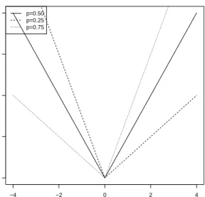
ρp(u) = u(p−I(u <0)), (1.2)

and I(·) is the indicator function. Equivalently, we can write (1.2) as

ρp(u) =

|u|+ (2p−1)u

2 .

Figure 1.1 shows the loss functions at three different quantiles, namelyp= 0.25, 0.50 and 0.75.

−4 −2 0 2 4 0.0 0.5 1.0 1.5 2.0 x loss function p=0.50 p=0.25 p=0.75

Figure 1.1. Loss function in (1.2) at different quantiles

Regularization, e.g. lasso (Tibshirani, 1996), is also adapted in QR to prevent over-fitting and improve prediction when the explanatory variables are high-dimensional (Li et al., 2010). This problem can be modified as an optimization over the quantile functions

fi =xiβ, i= 1, . . . , n for

n

X

i=1

ρp(yi−fi) +λ||f||q,

where f = (f1, . . . , fn) and || · ||q is the qth norm (Abeywardana and Ramos, 2015). For example, whenq = 1, this is the lasso penalty.

In Bayesian quantile regression, the coefficient β_p is sampled from its posterior distri-bution using the random walk Metropolis-Hastings algorithm (Yu and Moyeed, 2001) or Gibbs samplers (Tsionas, 2003). Li et al. (2010) studied Bayesian regularized quantile regression with the group lasso and elastic net penalty. Yu and Moyeed (2001) proposed that QR can be incorporated into Bayesian inference framework by assuming the error

terms follow the asymmetric Laplace distribution (ALD). Based on the ALD distributed error assumption, the likelihood function of β can be constructed, then its posterior distribution can be derived using Bayes’ theorem.

Asymmetric Laplace distribution

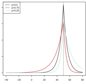
The probability density function (pdf) of an asymmetric Laplace distribution (ALD) is defined as f(x;µ, σ, p) = p(1−p) σ exp −(x−µ) σ [p−I(x≤µ)] , x∈(−∞,∞), (1.3)

where 0 < p < 1 is the skewness parameter, σ > 0 is the scale parameter, and µ ∈ _R

is the location parameter. The distribution ALD (x;µ, σ, p) has mean _E(x) = _p1−2₍₁₋p_p) and variance Var(x) = 1−2_p2₍₁₋p+2_p)p22. The corresponding CDF and quantile function are, respectively, F(x;µ, σ, p) =          pexp 1−_σp(x−mu), x≤µ, 1−(1−p) exp −_σp(x−µ), x > µ, (1.4) and F−1(x;µ, σ, p) =          µexp₁₋σ_p log(x_p), 0≤x < p, µ− σ p log −1−x 1−p , p < x≤1. (1.5)

As the pth quantile of the ALD distribution equals to the location parameter µ, i.e.

F−1(x;µ, σ, p)|x=p = µ, the ALD is used as the error distribution in quantile regression

−40 −20 0 20 40 60 80 0.00 0.02 0.04 0.06 0.08

ALD Density function

x

f(x)

p=0.5 p=0.75 p=0.25

Figure 1.2. Density of ALD with µ= 50, σ = 1, and p= (0.25, 0.5, 0.75)

The ALD can also be represented as a the mixture of an exponential and a normal distribution (Reed and Yu, 2009). If a variable follows the ALD in (1.3), we can represent as a location-scale mixture of normal distributions given by

=θz+τ√zu, (1.6) where θ = 1−2p p(1−p) and τ 2 ₌ 2 p(1−p).

1.1.1 Quantile regression under the asymmetric Laplace distributed error

Consider the model

where yi ∈ R is the response variable, xi ∈ Rk is the explanatory variable, βp ∈ Rk is the regression parameter for thepth quantile andi ∼ALD(0, σ, p) is the error term. By representing i as in (1.6), Equation (1.7) can be rewritten as

yi =x0iβp +θzi+τ

√

σziui, i= 1, . . . n, (1.8)

where ui ∼ N(0,1) and zi follows the exponential distribution with rate σ, e.g., exp(σ). Both θ and τ are constants with

θ = 1−2p

p(1−p) and τ

2 ₌ 2

p(1−p).

From (1.8), yi also follows an asymmetric Laplace distribution with location parameter xiβp, scale parameter σ and asymmetry parameter p, e.g., ALD(x0iβp, σ, p). The con-ditional distribution of yi given zi is a normal distribution with mean xiβp −θzi and variance τ2zi. The conditional density of y= (y1, . . . , yn)0 given z= (z1, . . . , zn)0 and βp

is f(y|β_p,z)∝(Πn_i=1z− 1 2 i ) exp −Πn_i=1(yi −x 0 iβp−θzi)2 2τ2_z i . (1.9)

Connection with Gibbs sampling

The conditional distribution p(zj|z−j,βp,y) is known as the full conditional in MCMC (Casella and George, 1992). The approximating density function in quantile regression can be derived from the full conditional distribution of variables in Gibbs sampling. We will first review quantile regression using Gibbs sampling which iteratively samples from the full conditional distributions.

Gibbs sampling for quantile regression

We first consider the model in (1.8). First we consider the quantile regression with the scale parameter σ fixed at σ = 1. Let the prior distribution be

β_p ∼N(µp0,Σp0), zi ∼exp(1). (1.10) The full conditional density of β_p can be shown as (Kozumi and Kobayashi, 2011)

βp|y,z∼N(µp,Σp), (1.11) where Σ−1_p = n X i xix0i τ2_z i + Σ−1_p0, (1.12) µ_p = Σp n X i=1 xi(yi−θzi) τ2_z i + Σ−1_p0µ_p0 ! . (1.13)

The full conditional density of zi, i = 1, ..., n is a generalized inverse Gaussian distribu-tion(Kozumi and Kobayashi, 2011)

zi|y,βp∼GIG( 1 2, ai, bi), (1.14) where ai = 2 + θ2 τ2 and bi = (yi−x0iβp)2 τ2 . (1.15)

The pdf of a generalized inverse Gaussian distribution is given by

f(p, a, b) = (a/b) p/2 2Kp( √ ab)x p−1 exp(−1 2(ax+b/x)), a >0, b >0, p∈R, (1.16)

whereKp(·)is the Bessel function of the third type. Next we extend our discussion to the more general case by treatingσ as an unknown variable and a prior is assigned to σ. The prior distribution forβ_p is the same as (1.11)

and a prior was given to σ

σ ∼IG(m0, n0), (1.18)

where IG(·) is the inverse gamma distribution. Similar to the previous situation, the posterior for β_p and z is the same as (1.11) and (1.14) respectively. The full conditional density forσ is then given by

σ|y,β_p,z∼IG(mp, np), (1.19) where mp = 3n+m0 np =n0+ n X i=1 (zi+ (yi−x0iβp−θzi)2 2τ2_z i )

Then the algorithm of Gibbs sampler iterates between the full conditional distribution of β_p given y, z, σ, the full conditional distribution of zi given y, βp, σ, and the full conditional distribution of σ given y, β_p, z. But this process can be time consuming when the parameter space is high dimensional and the data set is large.

Gibbs Sampling for quantile regression with the lasso penalty

The lasso regularization on quantile regression is brought up in Li and Zhu (2008), where the L1-norm penalty (lasso) is added to the minimization problem

min β n X i=1 ρp(yi−x0iβ) +λ k X i=1 |βi|.

Li et al. (2010) proposed an equivalent Bayesian formulation to the problem by putting a Laplace prior with mean zero and scale _λσ

j, j = 1, . . . , mon β p(β_p|σ,λ) = k Y j=1 λj σ exp(− λj σ|βj|), (1.20)

which leads to the posterior distribution p(β_p|y, σ,z)∝exp(−1 σ n X i=1 ρp(yi −x0iβp)− λj σ k X j=1 |βj|), (1.21)

where λj’s are the regularization parameter for corresponding regression coefficients βj. We put an inverse gamma prior onσ and a gamma prior on ηj =

λj

σ , j = 1, . . . , m. Let

s= (s1, . . . , sk) and the prior of βp can be further written as

p(β_p|σ,λ) = k Y j=1 λj σ exp −λj σ |βj| = k Y j=1 Z ∞ 0 1 √ aπsj exp −β 2 j 2sj _η2 j 2 exp −η 2 jsj 2 dsj. (1.22)

Then the full conditional distribution of βj isN(˜µj,ω˜j2), with

˜ µj = ˜ωj2 1 στ2 n X i=1 yi,jxi,jzi−1, (1.23) and ˜ ω_j−2 = 1 στ2 n X i=1 x2_i,jz_i−1+s−1_j , (1.24) where yi,j =yi−θzi− k X l=1,l6=j xi,lβl. (1.25)

The full conditional distribution of zi follows the same distribution as the previous case in (1.14), which is GIG(1₂,a˜i,˜bi), with

˜ ai = θ2 στ2 + 2 σ, (1.26) and ˜_{bj =} (yi −x0iβp)2 στ2 . (1.27)

The full conditional distribution for sj is given by p(sj|y,z,βp,s−j, τ, η2)∝p(βj|sj)p(sj|η2) ∝s−1_k /2exp{−1 2(η 2_s j+βj2s −1 j )}, (1.28) which is GIG(1₂, η2

j, βj2). The full conditional distribution for σ is also an inverse gamma distribution IG( ˜m,n˜), with ˜ m= 3n+m0, (1.29) and ˜ n=n0+ n X i=1 (zi+ (yi−x0iβp−θzi)2 2τ2_z i ). (1.30)

The full conditional distribution ofη2 _{follows a gamma distribution with shape parameter}

c+ 1 and rate parameter 1₂Pk

j=1sk+d, which is given by p(η2|y,z,β_p,s, σ)∝p(s|η2)p(η2) ∝(η2)k+c−1exp ( −η2 k X j=1 sk 2 +d !) , (1.31)

where cand d are constants given in the joint prior distribution of τ and η2

τ, η2 ∼τψ−1exp(−ξτ)(η2)c−1exp(−dη2). (1.32)

1.1.2 Variational inference

Variational inference is one of the popular methods to approximate intractable or difficult-to-compute posterior distributionsp(y|·) with an approximate posterior distributionq(y). Compared with MCMC such as Gibbs sampling, variational inference tends to be faster while achieves comparable prediction especially when dealing with large-scale data sets (Blei et al., 2016).

The idea of variational inference is to approximate the conditional density of latent vari-ables given observed varivari-ables using optimization. Let x = (x1, . . . , xn) be the set of observed variables and z= (z1, . . . , zm) be the set of latent variables. The joint density

of x and z is p(x,z). In the case that the conditional distribution p(z|x) is not directly

tractable, variational inference provides an alternative approach by approximating the conditional distribution p(z|x) using a tractable distribution q∗(z) ∈ Θ, where Θ is the family of densities over the latent variables. All density functionsq(z)∈Θ are candidate approximations to p(z|x). By solving the optimization problem, one can try to find the member in Θ that is the closest to p(z|x) in the Kullback-Leibler (KL) distance (Blei et al., 2016)

q∗(z) = argmin q(z∈Q)

KL q(z||p(z|x)), (1.33)

where KL(q(z)||p(z|x)) is the Kullback-Leiler distance between the posterior distribution

p(z|x) and the candidate distribution q(z) in the family Θ. It is defined as

KL q(z||p(z|x))=_E(logq(z))−_E(logp(z|x)), (1.34)

which is always non-negative (van Erven and Harremos, 2014). Wang and Blei (2018) gave the asymptotic properties of variational inference by proving that the posterior den-sity given by variational inference converges to the KL minimizer of a normal distribution centered at the truth. Zhang and Gao (2017) proved that the upper bound of the conver-gence rate, at which the variational posteriorq∗(z) converges to the true posterior p(z|x) is given by

2_n+ 1

nq(infz)∈Θp

(n)

where 2

n is the rate of convergence of the posterior distribution p(z|x). The second term is the variational approximation error with respect to Θ under p(₀n), where p(₀n) is the process that generates all the xi’s. If q(z) equals to the exact posterior distribution

p(z|x), the second term will be zero. The convergence rate will be the convergence rate

of the posterior distribution given by MCMC. In general, the second term in (1.35) 1

nq(infz)∈Θp

(n)

0 KL(q(z)||p(z|x))

is dominated by the first term 2

n in (1.35). Variational inference does not require the sampling process required in MCMC and Gibbs sampling. Hence, it provides computa-tional advantages without violating the asymptotic property of estimators in large-scale data set situations.

2. Variational inference for quantile regression

2.1 Algorithm of variational Bayes

Numerical implementation of the variational inference, the CAVI (coordinate ascent vari-ational inference) algorithm in Blei et al. (2016), is closely related to Gibbs sampling. In each iteration, CAVI optimizes every parameter sequentially, while keep others fixed. Finally, a local optimum is reached. Consider the model with parameter vector (latent variable)θ and observed variabley. Bayesian inference is based on the posterior density function

p(θ|y) = p(y,θ)

p(y) . (2.1)

Letq(·) be an arbitrary density function over the density family Θ. The logarithm of the marginal likelihood function satisfies

logp(y) = logp(y)

Z q(θ)dθ = Z q(β_p,z) log _p(y,β p,z)/q(βp,z) p(β_p,z|y)/q(β_p,z) dβ_pdz = Z q(β_p,z) log _p(y,β p,z) q(β_p,z) dβ_pdz+ Z q(β_p,z) log _q(β p,z) p(β_p,z|y) dβ_pdz ≥ Z q(β_p,z) log _p(y,β p,z) q(β_p,z) dβ_pdz, (2.2)

where θ = (β_p,z) and q(·) ∈ Θ is the candidate distribution used to approximate p(·). The above inequality holds because the second integral in (2.2)

Z q(β_p,z) log _q(β p,z) p(β_p,z|y) dβ_pdz, (2.3)

is the KL distance between q(β_p,z) and p(β_p,z|y), which is always non-negative by definition (Kullback and Leibler, 1951). The equality holds if and only if q(β_p,z) =

p(β_p,z|y). Under this special case, the estimation of variational inference will coincide

with the estimation given by Gibbs sampling. Recall from Equation (1.33), that the goal of variational inference is to find the distribution q(·) that is closest to the conditional distribution p(θ|y) in KL distance. According to (2.2), minimizing the KL distance in (2.3) between q(β_p,z) and p(β_p,z|y) is equivalent to maximizing the lower bound

L= Z q(β_p,z) log _p(y,β p,z) q(β_p,z) dβ_pdz. (2.4)

In variational inference, the assumption of the complexity of the density family Θ deter-mines the complexity of optimization problem. In themean-filed variational family (a.k.a.

naive mean approach) (Blei et al., 2016), where the latent variablesθ are assumed to be mutually independent and governed by distinct factors in the variational densityq(θi), is used to approximate the conditional distribution p(θi|y,θ−i). e.g.

q(θ) = n

Y

i=1

q(θi),

where each latent variable θi is governed by its own variational factor. One can also use other approximations such as generalized mean field (Blei et al., 2016), in which the

parameters of interest are divided into groups and the parameters inside each group are allowed to be dependent. e.g.

q(θ) = n

Y

i=1

q(θi1, . . . , θim).

In this thesis, we adopt themean-field variational family approach, by assuming indepen-dence between latent variablesβ_p and z. Then the log-likelihood function can be written as Z q(β_p,z) log{p(y,βp,z) q(β_p,z) }dβpdz= Z q(β_p)q(z) log{p(y|βp,z)p(βp)p(z) q(β_p)q(z) }dβpdz = Z q(β_p)q(z) log{p(y|β_p,z)}dβ_pdz + Z q(β_p) log{p(βp) q(β_p)}dβp + Z q(z) log{p(z) q(z)}dz, (2.5)

where q(·) is the candidate density from the density family Θ. Consider thejth variable

zj in the latent variable z. The conditional density of zj conditioning on all other latent variables and observed variables is

p(zj|z−j,βp,y),

where z−j = (z1, . . . , zj−1, zj+1, . . . , zn). Then one can fix all other variational factors in z−j, and maximize the lower bound of this conditional distribution with respect to the density of zj. The optimal qj∗(zj)∈Θj is proportional to the exponential of the expected log conditional density (Blei et al., 2016)

q∗(zj)∝exp(E−j(logp(zj|y,z−j))). (2.6)

The latent variables are updated successively using (2.6). The iteration stops when the difference between two sequential lower bound is negligible. i.e., smaller than a

prespec-ified tolerance level. Algorithm: (CAVI)

Step1 Initialize q(θ)

Step2 Update q(zj)∗, j = 1, . . . , nand q(βp) by

q∗(zj)∝exp(E−j(logp(zj|y,z−j))),

.. .

q(βp)∝exp(Ez(logp(βp|y,z)))

Step3 Update the lower bound L, repeat step 2 and 3 until the change in L is negligible.

2.2 Variational inference for quantile regression without regularization

We start from the simplest case, where the scale parameter is fixed at σ= 1. Then only β_p and zneed to be updated in the iterations of variational inference.

The optimal approximation density function q∗(β_p) is given by

with logp(β_p|y,z) =−1 2  log(2π) + log  det n X i=1 xix0i τ2_z i + Σ−1_p0 !−1    − 1 2(βp−µp0) 0 n X i=1 xix0i τ2_z i + Σ−1_p0 ! (β_p−µ_p0) =−1 2log  det n X i=1 xix0i τ2_z i + Σ−1_p0 !−1  − 1 2β 0 p n X i=1 xix0i τ2_z i + Σ−1_p0 ! β_p +β0_p n X i=1 xi(yi−θzi) τ2_z i + Σ−1_p0µp0 ! − 1 2 n X i=1 xi(yi−θzi) τ2_z i + Σ−1_p0µp0 !0 _n X i=1 xix0i τ2_z i + Σ−1_p0 !−1 _n X i=1 xi(yi−θzi) τ2_z i + Σ−1_p0µ_p0 ! +const. (2.7) The expectation of logp(βp|y,z) is with respect to zi, where zi follows the generalized inverse Gaussian distribution GIG(1₂, aqi, bqi), with

E(zi) = p bqiK3/2( p aqibqi) √ aqiK1/2( p aqibqi) , E(1 zi ) = √ aqiK3/2( p aqibqi) p bqiK1/2( p aqibqi) − 1 bqi , and E(lnzi) = ln p bqi √ aqi + ∂ ∂plnKp( p aqibqi),

where Kp(·) is the Bessel function with order p. The approximation of the expectations could be used for simplicity in some situations (Abeywardana and Ramos, 2015), with

E(zi) =

s

bqi

aqi

and E(1 zi ) = r_a qi bqi − 1 bqi . (2.9)

In general the exact values of these expectations are preferred, as the approximated value might cause convergence problems. e.g., the value of the lower bound sometimes diverges if the approximated values are used. The expectation of the logarithm of the full conditional density logp(β_p|y,z) is

Ez(logp(βp|y,z)) =β0p( n X i=1 xiyi τ2 E( 1 zi )− n X i=1 θ τ2xi+ Σ −1 p0µp0) −1 2β 0 p( n X i=1 xix0i τ2 E( 1 zi ) + Σ−1_p0)β_p +const. (2.10)

Taking exponential of the expectation _Ez(logp(βp|y,z)), we then see that the density

function of q(β_p) is for the multivariate normal distribution N(µq,Σq), with

Σq = n X i=1 xix0i τ2 E 1 zi + Σ−1_p0 !−1 , (2.11) and µq = Σq n X i=1 xiyi τ2 E 1 zi − n X i=1 θ τ2xi+ Σ −1 p0µp0 ! . (2.12)

The pdf of q(zi)’s are calculated in a similar manner as

q(zi)∝exp(Eβp(logP(zi|y,βp))), (2.13) where logp(zi|y,βp) = − 1 2log(zi)− 1 2(aizi+bi/zi) +const. (2.14)

The expectation of the log conditional density logp(zi|y,βp) with respect to βp follows the GIG distribution

q(zi)∼GIG( 1 2, aqi, bqi), (2.15) with aqi = 2 + θ2 τ2, (2.16) and bqi = y2 i −2yix0iµq+x 0 i(µqµ 0 q+ Σq)xi τ2 . (2.17)

The µq and Σq in (2.17) are the mean and variance of q(βp), which are given in (2.11)

and (2.12). From (2.4), the lower bound is given by

E(logp(y|θ)) +E(log(p(θ)))−E(log(q(θ))), (2.18)

with θ = (z,β_p). Then the lower boundl is

l= Z q(z)q(β_p) log p(y|z,β_p)dzdβ_p+ Z q(z) log (p(z)/q(z))dz + Z q(β_p) log(p(β_p)/q(β_p))dβ_p =_Eq(z),q(βp)log (y|z,βp) +_Eq(z)log(p(z))−Eq(z)log(q(z)) +_Eq(βp)log(p(βp))−Eq(βp)log(q(βp)). (2.19)

The variational inference algorithm when σ= 1 is Algorithm 1:

Step1 Initialize mean µ_q and covariance matrix Σq.

Step2 Repeat Steps 3-5 if the absolute change in lower boundl ≥t, wheretis the tolerance given, e.g. t= 10−5.

Step3 Update parameters in q(z). q(zi)∼GIG(1₂, aqi, bqi), where aqi = 2 + θ2 τ2, bqi = y2 i −2yix0iµq+x 0 i(µqµ 0 q+ Σq)xi τ2 .

Step4 Update parameters in q(β_p). q(β_p)∼N(µq,Σq), where

Σq = n X i=1 xix0i τ2 E 1 zi + Σ−1_p0 !−1 µq = Σq n X i=1 xiyi τ2 E 1 zi − n X i=1 θ τ2xi+ Σ −1 p0µp0 ! .

Step5 Update lower bound l

l=_Eq(z),q(βp)(y|z,βp) +Eq(z)log(p(z))−Eq(z)log(q(z))

+_Eq(βp)log(p(βp))−Eq(βp)log(q(βp))

When the scale parameterσ is taken into account, similar as the case in Gibbs sampling, a prior distribution of σ is assumed and we update the value of β_p, z and σ successively in the iteration of variational inference. The approximation distribution of β_p, z and σ

are given by

q(β_p)∼N(µ_q,Σq), (2.20)

q(zi)∼GIG(aqi, bqi), (2.21)

and

with Σq = n X i=1 xix0i τ2 E 1 zi E 1 σ + Σ−1_p0 !−1 , (2.23) µq = Σq Q_E 1 σ + Σ−1_p0µ_p0 , (2.24) aqi = 2 + θ 2 τ2 E 1 σ , (2.25) bqi = M τ2E 1 σ , (2.26) mq = 3n+m0, (2.27) and nq =n0+ n X i=1 E(zi) +N. (2.28)

The Q in Equation (2.24) is given by

Q= ( n X i=1 xiyi τ2 E( 1 zi )− n X i=1 θ τ2xi). (2.29)

The M is Equation (2.26) is given by

M=y2_i −2yix0iµq+x

0

i(µqµ

0

q+ Σq)xi. (2.30)

The N in Equation (2.28) is given by

N= n X i=1 M 2τ2E 1 zi −θ(yi−x 0 iµp) τ2 + θ2 2τ2E(zi). (2.31) Algorithm 2:

Step1 Initialize mean µ_q and covariance matrix Σq.

Step3 Update parameters in q(z), usingq(zi)∼GIG(1₂, aqi, bqi).

Step4 Update parameters in q(β_p), using q(β_p)∼N(µq,Σq).

Step5 Update parameters in q(σ), usingq(σ)∼IG(mq, nq).

Step6 Update the lower bound l

2.3 Variational inference for quantile regression with the lasso penalty

The approximation density function q(·) is calculated using the same method given in Section (2.2)

q(θi)∝exp(Eθ−i(logp(θi|θ−i))), (2.32)

where θ−i is the vector of variables without the ith variable θi. The density function of q(βj) follows the normal distribution

N(µqj, ωqj), (2.33) with ω_q−2 j = E(1/σ) τ2 n X i=1 x2_i,jE(1/zi) +E(1/sj), (2.34) and µqj =ω 2 qj E(1/σ) τ2 n X i=1 xi,j yiE 1 zi −θ− k X l=1,l6=j xi,lµqjE 1 zi !! , (2.35) where _E(1/σ) = mq

nq with mq and nq given in (2.44) and (2.45). The density function of

q(zi) follows the generalized inverse Gaussian

GIG(1

with aqi = θ2 τ2 + 2 E 1 σ , (2.37) and bqi = (y2 i −2yix0iµq+x 0 iE(βpβ 0 p)xi)E(σ1) τ2 . (2.38)

The density functions ofq(sj) and q(η2) follow the generalized inverse Gaussian

GIG(1 2, η 2 qj, β 2 qj), (2.39)

and the Gamma distribution

Gamma k+c, k X j=1 E(sj) 2 +d ! , (2.40) respectively, with η_q2_j =_E(η2) = k+c Pk j=1 E(sj) 2 +d , (2.41) and β_q2 j =E(β 2 j) = µ 2 qj +ω 2 qj. (2.42)

The density function ofq(σ) follows the inverse Gamma distribution

IG(mq, nq), (2.43) with mq = 3n+m0, (2.44) and nq=n0+ n X i=1 1 + θ 2 2τ2 E(zi) + E(yi−xiβp)2 2τ2 E 1 zi − E(yi−xiβ) τ2 θ . (2.45)

Algorithm 3:

Step1 Initialize parameters in the prior distribution, including m0, n0, c and d.

Step2 Initialize mean µ_q and covariance matrix Σq.

Step3 Update parameters in q(σ), usingq(σ)∼IG(mq, nq).

Step4 Update parameters in q(sj), usingq(sj)∼GIG(1₂, ηq2j, β

2

qj).

Step5 Update parameters in q(η2), using q(η2)∼Gamma(k+c,Pk

j=1

E(sj)

2 +d).

Step6 Update parameters in q(z), usingq(zi)∼GIG(1₂,˜aqi,˜bqi).

Step7 Update parameters in q(β_p), using q(βj)∼N(µqj, ωqj).

Step8 Update the lower boundl, if the difference between two consecutivelis bigger than the tolerance level specified, repeat Steps 3 ∼8.

3. Simulation studies

We compare the variational inference with the Gibbs sampling method in terms of accu-racy and speed using simulated data. CPU time is used to measure the speed of different algorithms and predictive mean squared error (MSE) is used to measure the accuracy. As-suming independent and identically (i.i.d) distributed errors, we conduct the simulation using the following models.

1. Sparse case with Gaussian noise: β1 = (3,1.5,0,0,2,0,0,0), i ∼N(0,0.62).

2. Dense case with Gaussian noise:β2 = (0.85,0.85,0.85,0.85,0.85,0.85,0.85,0.85), i ∼

N(0,0.62).

3. Very sparse case with Gaussian noise: β3 = (2,4,0, . . . ,0 | {z } 10 ), i ∼N(0,0.62). 4. High-dimensional: β4 = (2, . . . ,2 | {z } 40 ,0, . . . ,0 | {z } 40 ,3, . . . ,3 | {z } 40 ),i ∼N(0,0.62)

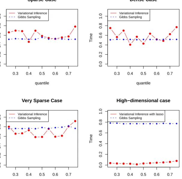
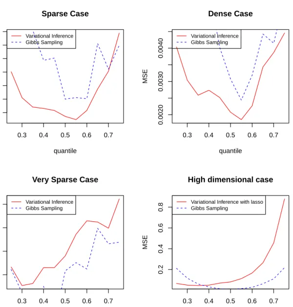
For first three models, we set the sample sizen equal to 1000. And the sample size for the last model is 50. In model 1∼3 we run the regression using variational inference without the lasso penalty (Algorithm 2). And variational inference with the lasso penalty is applied in the high-dimensional case. Gibbs sampling are applied in all four cases for comparison. Fig. 3.1 and Fig. 3.2 show the CPU time and predictive MSE using varia-tional inference and Gibbs sampling under different quantiles, respectively.

● ● ● ● ● ● ● _● ● ● ● 0.3 0.4 0.5 0.6 0.7 0.0 0.2 0.4 0.6 0.8 1.0 Sparse Case quantile Time Variational Inference Gibbs Sampling ● ● ● ● ● ● ● ● ● ● ● 0.3 0.4 0.5 0.6 0.7 0.0 0.2 0.4 0.6 0.8 1.0 Dense Case quantile Time Variational Inference Gibbs Sampling ● ● ● ● ● ● ● ● ● ● ● 0.3 0.4 0.5 0.6 0.7 0.0 0.2 0.4 0.6 0.8 1.0

Very Sparse Case

quantile Time Variational Inference Gibbs Sampling ● ● ● ● ● ● ● ● ● ● ● 0.3 0.4 0.5 0.6 0.7 0.0 0.2 0.4 0.6 0.8 1.0 High−dimensional case quantile Time

Variational Inference with lasso Gibbs Sampling

0.3 0.4 0.5 0.6 0.7 0.0025 0.0035 0.0045 0.0055 Sparse Case quantile MSE Variational Inference Gibbs Sampling 0.3 0.4 0.5 0.6 0.7 0.0020 0.0030 0.0040 Dense Case quantile MSE Variational Inference Gibbs Sampling 0.3 0.4 0.5 0.6 0.7 0.006 0.007 0.008 0.009

Very Sparse Case

quantile MSE Variational Inference Gibbs Sampling 0.3 0.4 0.5 0.6 0.7 0.2 0.4 0.6 0.8

High dimensional case

quantile

MSE

Variational Inference with lasso Gibbs Sampling

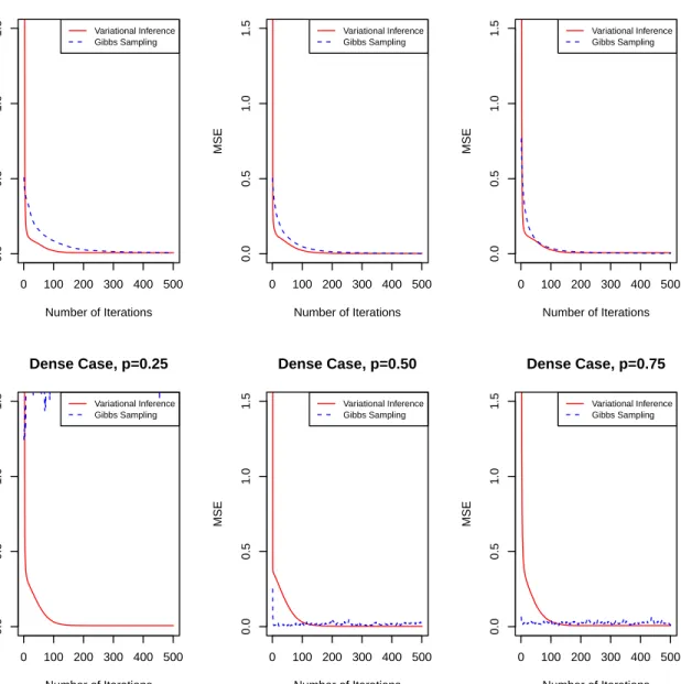
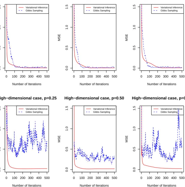
packagebayesQR (Benoit and den Poel, 2017). In the sparse and dense case, variational inference has a comparable speed compared with Gibbs sampling, but variational infer-ence maintains a lower MSE. Variational inferinfer-ence tends to need more time for extreme quantiles. In the very sparse case and the case when predictor is more than sample size, variational inference spends less time than quantile regression but has a slightly larger MSE. Variational inference could be used as a faster alternative to Gibbs sampling when the dimension of the predictor is high, while provides a comparable accuracy in terms of MSE. We also compare the number of iterations needed to converge using quantile re-gression with the lasso penalty and Gibbs sampling under quantile p ={0.25,0.5,0.75}. The results are shown in Fig. 3.3 and Fig. 3.4. It shows that the two methods take almost the same number of iterations to converge. However, turning points of variational inference usually occur before that in Gibbs sampling, which indicates that the declining of MSE in variational inference is usually faster in the first few iterations.

0 100 200 300 400 500 0.0 0.5 1.0 1.5 Sparse Case, p=0.25 Number of Iterations MSE Variational Inference Gibbs Sampling 0 100 200 300 400 500 0.0 0.5 1.0 1.5 Sparse Case, p=0.50 Number of Iterations MSE Variational Inference Gibbs Sampling 0 100 200 300 400 500 0.0 0.5 1.0 1.5 Sparse Case, p=0.75 Number of Iterations MSE Variational Inference Gibbs Sampling 0 100 200 300 400 500 0.0 0.5 1.0 1.5 Dense Case, p=0.25 Number of Iterations MSE Variational Inference Gibbs Sampling 0 100 200 300 400 500 0.0 0.5 1.0 1.5 Dense Case, p=0.50 Number of Iterations MSE Variational Inference Gibbs Sampling 0 100 200 300 400 500 0.0 0.5 1.0 1.5 Dense Case, p=0.75 Number of Iterations MSE Variational Inference Gibbs Sampling

0 100 200 300 400 500

0.0

0.5

1.0

1.5

Very Sparse Case, p=0.25

Number of Iterations MSE Variational Inference Gibbs Sampling 0 100 200 300 400 500 0.0 0.5 1.0 1.5

Very Sparse Case, p=0.50

Number of Iterations MSE Variational Inference Gibbs Sampling 0 100 200 300 400 500 0.0 0.5 1.0 1.5

Very Sparse Case, p=0.75

Number of Iterations MSE Variational Inference Gibbs Sampling 0 100 200 300 400 500 0.0 0.5 1.0 1.5 High−dimensional case, p=0.25 Number of Iterations MSE Variational Inference Gibbs Sampling 0 100 200 300 400 500 0.0 0.5 1.0 1.5 High−dimensional case, p=0.50 Number of Iterations MSE Variational Inference Gibbs Sampling 0 100 200 300 400 500 0.0 0.5 1.0 1.5 High−dimensional case, p=0.75 Number of Iterations MSE Variational Inference Gibbs Sampling

4. Conclusions

This thesis derive the variational inference algorithm for quantile regression with and without the lasso regularization. Simulated studies show that, in comparison with Gibbs sampling, variational inference has a faster MSE declining within few iterations. Usually variational inference could maintain a comparable accuracy with Gibbs sampling. In very sparse data sets and the case when predictor is more than sample size, variational inference could usually perform better without sacrificing significant accuracy.

REFERENCES

S. Abeywardana and F. Ramos. Variational inference for nonparametric bayesian quan-tile regression. pages 1686–1692, 2015.

G. Bassett and H.-L. Chen. Portfolio style: Return-based attribution using quantile regression. Empirical Economics, 26:293–305, 2001.

D. Benoit and D. V. den Poel. bayesqr: A Bayesian approach to quantile regression.

Journal of Statistical Software, 76(7):1–32, 2017.

D. M. Blei, A. Kucukelbir, and J. D. McAuliffe. Variational inference: A review for statisticians. arXiv e-prints, 2016.

G. Casella and E. I. George. Explaining the Gibbs sampler. The American Statistician, 46(3):167–174, 1992.

R. Koenker and G. Bassett. Regression quantiles. Econometrica, 46(1):33–50, 1978.

R. Koenker and O. Geling. Reappraising medfly longevity: A quantile regression survival analysis. Journal of the American Statistical Association, 96(454):458–468, 2001.

H. Kozumi and G. Kobayashi. Gibbs sampling methods for Bayesian quantile regression.

S. Kullback and R. A. Leibler. On information and sufficiency. The Annals of Mathe-matical Statistics, 22(1):79–86, 03 1951.

Q. Li, R. Xi, and N. Lin. Bayesian regularized quantile regression. Bayesian Analysis, 5(3):533–556, 09 2010.

Y. Li and J. Zhu. L1-norm quantile regression. Journal of Computational and Graphical Statistics, 17(1):163–185, 2008.

G. R. Pandey and V.-T.-V. Nguyen. A comparative study of regression based methods in regional flood frequency analysis. Journal of Hydrology, 225:92–101, 1999.

C. Reed and K. Yu. A partially collapsed Gibbs sampler for Bayesian quantile regression. 01 2009.

R. Tibshirani. Regression shrinkage and selection via the lasso. Journal of the Royal Statistical Society, 58(1):267–288, 1996.

E. Tsionas. Bayesian quantile inference. Journal of Statistical Computation and Simu-lation, 73(9):659–674, 2003.

T. van Erven and P. Harremos. Renyi divergence and Kullback-Leibler divergence. IEEE Transactions on Information Theory, 60(7):3797–3820, 2014.

Y. Wang and D. M. Blei. Frequentist consistency of variational Bayes. Journal of the American Statistical Association, pages 1–15, 2018.

K. Yu and R. A. Moyeed. Bayesian quantile regression. Statistics & Probability Letters, 54(4):437–447, 2001.

F. Zhang and C. Gao. Convergence rates of variational posterior distributions. arXiv e-prints, 2017.