LAP-based motion-compensated frame interpolation

(1)

c

(2)

LAP-BASED MOTION-COMPENSATED FRAME INTERPOLATION

BY

TEJAS JAYASHANKAR

THESIS

Submitted in partial fulfillment of the requirements

for the degree of Bachelor of Science in Electrical and Computer Engineering in the Undergraduate College of the

University of Illinois at Urbana-Champaign, 2019

Urbana, Illinois

Adviser:

(3)

ABSTRACT

High-quality video frame interpolation often necessitates accurate motion es-timates between consecutive frames. Standard video encoding schemes often estimate the motion between frames using variants of block matching algo-rithms. For the sole purposes of video frame interpolation, more accurate estimates can be obtained using modern optical flow methods.

In this thesis, we use the recently proposed Local All-Pass (LAP) algorithm to compute the optical flow between two consecutive frames. The resulting flow field is used to perform interpolation using cubic splines. We com-pare the interpolation results against a well-known optical flow estimation algorithm as well as against a recent convolutional neural network scheme for video frame interpolation. Qualitative and quantitative results show that the LAP algorithm performs fast, high-quality video frame interpolation, and perceptually outperforms the neural network and the Lucas-Kanade method on a variety of test sequences. We also perform a case study to compare LAP interpolated frames against those obtained using two leading methods on the Middlebury optical flow benchmark. Finally, we perform a user study to gauge the correlation between the quantitative and qualitative results.

Keywords: Motion Compensation, Frame Interpolation, Optical Flow, Splines, Convolutional Neural Network, Adaptive Separable Convolution, Lucas-Kanade algorithm, Local All-Pass filters

(4)

ACKNOWLEDGMENTS

I would like to express my deepest appreciation for my advisor and mentor, Professor Pierre Moulin, who has provided me with guidance, support and invaluable research experience during the course of our research project. Ever since our first conversation in my freshman year, I knew that I would have the ability to deepen my knowledge and become an independent researcher by working with Professor Moulin. During the course of our research project, I have expanded my understanding of signal processing, statistical inference and machine learning. These skills have proven not only valuable for my work here at UIUC, but they will also play an important role during my future research internships and for my Ph.D.

I am also very fortunate to author a paper with Professor Moulin, Professor Thierry Blu and Dr. Christopher Gilliam, that has been submitted to the IEEE Conference for Image Processing (ICIP 2019). I would like to also express my deepest appreciation for Professor Thierry Blu at the Chinese University of Hong Kong and Dr. Christopher Gilliam at RMIT University, Melbourne for their valuable inputs while writing the paper and for sharing code that was used during the initial development of the LAP algorithm. Professor Moulin was very supportive during the conference paper submis-sion phase and gave me constructive feedback that I will forever remember while writing a research paper.

I would also like to thank all my other professors and staff at UIUC who have made the past four years a fun, energetic and unforgettable experience. I would like to especially thank Professor Radhakrishnan for his invaluable support and mentorship over the past few years. I have not only learned from my professors, but also from my friends. I am glad to have made so many caring and motivated friends during my time here and it is the daily

(5)

interactions with them that make college so much more fun and lively. I would also like to thank my family for all the love, care and support that they have given me. I would like to especially thank my parents and my sister, Bhavya, for moving half way across the world to help me achieve my dream of studying in the US. I would like to especially thank my dad, the most hard-working person I know, and it is his hard work and motivating spirit that allow me to study at a top-notch university. Without my mom’s love, hard work, support and tasty food, my experience at UIUC would be bland. My sister constantly reminds me to have fun while working and I am truly grateful for her love and companionship. Finally, I would like to thank my grandparents who have encouraged me from a young age to achieve my goals and aspirations.

(6)

LIST OF TABLES

2.1 Operation count for Lucas-Kanade to interpolate single

frame of size 1024x640. . . 13 3.1 Operation count for Adaptive Separable Convolution to

interpolate single frame of size 960×540×3. . . 27 4.1 Operation count for LAP to interpolate a single frame of

size 960x540x3. Below, ma stands for multiply-adds and the cleaning procedures involve NaN inpainting, mean and median filtering. Flow estimation requires 3 subtractions,

2 divisions and 1 addition per pixel. . . 36 5.1 MSE evaluation on the Middlebury dataset (high-speed

camera samples). Bold values indicate best results. . . 38 5.2 Average interpolation MSE on Derf’s Media Collection.

Bold values indicate best results. . . 40 5.3 Average interpolation MSE on EPIC Kitchens dataset. Bold

values indicate best results. . . 42 5.4 Execution times and MSE of the various optical flow

meth-ods and CNN on the basketball sequence. All times are in

seconds. . . 43 5.5 Number of operations (multiply-adds) and execution time

(CPU) required to interpolate a frame of size 960x540x3. Execution time is in seconds, measured on a machine with Intel Core i7-8750H processor and 32 GB RAM. The ex-ecution time for the CNN was extrapolated based on the

(9)

LIST OF FIGURES

2.1 Block matching a block of width 16 pixels within a search

radius of 7 pixels. . . 5

2.2 Illustration of Three-Step Search. . . 7

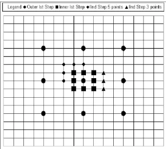
2.3 Illustration of New Three Step Search. If minimum occurs at a corner pixel five additional points are added (squares) else three additional points are added (triangles). . . 8

2.4 Illustration of Four Step Search. . . 10

2.5 Lorentzian norm and `2 norm. . . 16

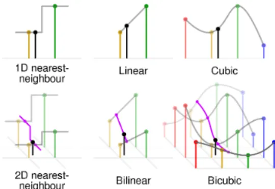
3.1 Illustration of different interpolation techniques. . . 22

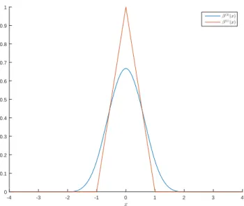
3.2 Linear and cubic elementary B-splines. . . 23

3.3 Cubic B-spline and OMOMS comparison. . . 24

3.4 Illustration of neural network architecture. Given input framesI1 and I2, an encoder-decoder network extracts fea-tures that are given to four sub-networks that each estimate one of the four 1D kernels for each output pixel in a dense pixel-wise manner. The estimated pixel-dependent kernels are then convolved with the input frames to produce the interpolated frame Iint. . . 26

4.1 Estimated flow using different methods. A radius of 10 was used for LK and HS. HS required 250 iterations for convergence. LAP flow was estimated using all six basis filters. 33 5.1 Beanbags sequence: The original sequence is shown at the top. The original second frame is shown in (a), the LAP-interpolated second frame is shown in (b), the CNN-interpolated second frame is shown in (c), the LK-CNN-interpolated second frame is shown in (d). LAP was used to compute the optical flow in (a), (b) and (c). . . 39

(10)

5.2 Soccer sequence: The original sequence is shown at the top. Original frame 314 is shown in (a), LAP-interpolated frame 314 is shown in (b), CNN-interpolated frame 314 is shown in (c) and the LK interpolated 314 is shown in (d). The optical flow between frame 314 and frame 314 is shown for the original sequence in (a) and for the three methods in the other columns. LAP was used to compute the optical

flow in (a), (b) and (c). . . 41 5.3 Basketball sequence (frames 9, 10, 11): The original

se-quence is shown at the top. The original sese-quence is shown in (a). In (c) DF2 stands for Deepflow2 and in (e) MDPF2 stands for MDP-Flow2. Flow fields between frame 1 and

frame 2 is shown at the bottom. . . 43 5.4 Results of the user study on 10 different sequences. The

sequences reported here best illustrate the discrepancy

(11)

LIST OF ABBREVIATIONS

Abbreviation Expansion

4SS Four-Step Search

ARPS Adaptive Rood Pattern Search

BA Black and Anandan

CNN Convolutional Neural Network

FRUP Frame-Rate Up-Conversion

FS Full Search

HS Horn-Schunck

LAP Local All-Pass

LK Lucas-Kanade

MCFI Motion-Compensated Frame Interpolation

MC-FRUP Motion-Compensated Frame-Rate Up-Conversion MOMS Maximal-Order Interpolation of Minimal Support

NTSS New Three-Step Search

OMOMS Optimal Maximal-Order Interpolation of Minimal Sup-port

PF Poly-Filter

(12)

CHAPTER 1 INTRODUCTION

1.1 Background

1.1.1 Motion-Compensated Frame Interpolation

Frame-Rate Up-Conversion (FRUC) is the process by which new intermedi-ate frames are inserted into a video sequence with the goal of improving the temporal resolution (frame-rate) of the video sequence. These intermediate frames are generated by only using the frames in the original video. These intermediate frames could be a copy of one of the original frames in the se-quence or they could be newly generated frames.

FRUC plays a pivotal role in video processing and has many applications to various fields. In a video coding and compression setup, with a limited bit transmission rate, the system is constrained by memory and processing power. FRUC can not only be used to interpolate between the input frames, but an advanced algorithm can also accurately estimate the displacement fields, which can then be transmitted. In [1], Krishnamurthyet al. encode the displacement field of a subsampled video using a block-matching approach under bit constraints. The decoder performs motion-compensated FRUC (MC-FRUC) to interpolate new frames using bidirectional predictions to tackle occlusions. Literature that covers FRUC for compressed video can also be found in [2, 3]. In this thesis we specifically study motion-compensated frame interpolation (MCFI), wherein the frame-rate is increased through the interpolation of new frames.

Frame interpolation might still be desired even if the system is equipped with high transmission rates and large memory bandwidth. MCFI has been

(13)

used for interpolation in echocardiographical video sequences [4]. Instead of interpolating a single frame, multiple frames are interpolated between a pair of images to augment the observable ventricular functions and better visualize cardiac dynamics. Image registration techniques are used for mo-tion estimamo-tion and dimensionality reducmo-tion is employed to optimize for the number of intermediate frames to produce. It should also be noted that many MCFI algorithms are specifically designed for the underlying system that it is deployed on [5].

1.2 Thesis Objectives

In this thesis we use the recently developed Local All-Pass (LAP) algorithm for optical flow estimation to perform motion estimation. These motion es-timates are then used to create an interpolated frame using cubic splines. We compare the interpolation results against the Lucas-Kanade method, a standard optical flow algorithm and a recently proposed convolutional neural network (CNN) approach for video-frame interpolation based on separable filter estimation.

The interpolated frames are evaluated quantitatively using the Mean-Squared Error (MSE) [6] and qualitatively by observing the interpolated frames. A detailed analysis of the interpolation quality is performed and finally a user study is conducted to further understand the correlation between MSE and subjective visual quality.

1.3 Organization of Thesis

This thesis is organized into six different chapters as follows:

1. Chapter 1 introduces the MCFI problem and details the organization of the thesis.

2. Chapter 2 is concerned with motion estimation. Section 2.1 covers state-of-the-art block matching algorithms for motion estimation. Sec-tion 2.2 introduces five standard optical flow algorithms for moSec-tion estimation.

(14)

3. Chapter 3 explains the MCFI problem statement and covers various interpolation algorithms used for interpolating between signals. Sec-tion 3.3 briefly explains a new convoluSec-tional neural network for frame interpolation.

4. Chapter 4 explains the Local All-Pass (LAP) algorithm for motion estimation. The main principles and algorithm details are explained. 5. Chapter 5 reports interpolation results on three different datasets. It

also includes results from a user study performed to understand the correlation between MSE and visual quality.

6. Chapter 6 concludes the thesis and contains final remarks on the ex-periments and results.

(15)

CHAPTER 2 MOTION ESTIMATION

Motion estimation has been a hot research topic since the 1970s. Many of the original and currently used video coding standards use motion estimation to encode and decode information [7, 8]. Motion estimation between images is often computed in two different ways:

1. Block Matching: The images are broken up into blocks (also called macro-blocks), which is essentially a cluster of pixels. Typical block sizes are 4x4, 8x8 and 16x16. The best matches in relation to some error metric, between corresponding blocks in both images, are used to estimate the motion vectors.

2. Optical Flow: The motion between a pair of images is estimated for each pixel. Optical flow motion estimates tend to be much more ac-curate than block matching motion vectors. However, these methods also tend to be much more complex and computationally expensive. In the next few sections we will review literature that discusses block-matching and optical flow methods for motion estimation.

2.1 Block Matching

Block matching algorithms implicitly assume that objects and patterns vary in position between images but remain structurally similar. The idea is to divide the images into blocks of size n×n where n is typically 4, 8 or 16. The illustration in 2.1 is taken from [9] and it shows a typical block size. For each block B1 ∈ B in I1, where B is the space of all blocks, the

corresponding block B2 in image I2 can be found by minimizing some error

(16)

Figure 2.1: Block matching a block of width 16 pixels within a search radius of 7 pixels.

the Mean Absolute Error (MAE). The formula for these criteria between two

M ×N matrices is given below:

MSE(x, y) = 1 M N M X i=1 N X j=1 (x(i, j)−y(i, j))2, (2.1) MAE(x, y) = 1 M N M X i=1 N X j=1 |x(i, j)−y(i, j)|. (2.2) Most algorithms also restrict the search radius to be within p pixels from the center of the current block under consideration as is shown in Figure 2.1. This is done for two reasons:

1. For faster computation. Searching over the whole image can be com-putationally intensive. Moreover, it lengthens the execution time. 2. In most situations, especially MCFI, assumptions on the velocity of

the object can be made to ensure that the highest correlation between blocks only occurs within a fixed radius with high probability. This is because most natural occurring scenes have generally smoothly varying motion.

In the next few subsections we will briefly review commonly used block-matching algorithms for motion estimation. A more in-depth treatment of these algorithms can be found in [9, 10].

(17)

2.1.1 Full Search

In Full Search (FS), every block between I1 and I2 is compared within a

search window. For every block in I1, the block in I2 that results in the

lowest MSE is chosen. Let the images be broken up into blocks of sizeK×K

and let the search window radius be p pixels. Then, the number of blocks,

n, compared for each reference block is:

n= 4p2. (2.3)

Thus, the total number of operations performed is:

ops =n×K2 =O((pK)2). (2.4) FS gives the best match amongst all block matching algorithms for the same block width and search window radius. However, this comes at the cost of increased computational complexity and longer execution time.

2.1.2 Three-Step Search

The Three-Step Search (TSS) block matching algorithm [9] is one of the first block matching algorithms introduced and it forms the basis for many more complex block matching algorithms. Instead of searching all blocks within a window, TSS employs a much more strategic algorithm to find the best match for a reference frame while also reducing the time complexity. TSS finds a matching block in three steps.

1. Step 1: Match the central block and all blocks at a distance of 4 pixels away from the center of the reference block,x. Choose the central pixel of the matched block with lowest MSE. Call this position x1.

2. Step 2: Reduce the search radius from 4 pixels to 2 pixels. Now match all blocks at a distance of 2 pixels fromx1to the reference block. Choose

the central pixel of the matched block with the lowest MSE. Call this position x2.

3. Step 3: Reduce the search radius from 2 pixels to 1 pixel. Now match all blocks at a distance of 1 pixel fromx2 to the reference block. Choose

(18)

Figure 2.2: Illustration of Three-Step Search.

the central pixel of the matched block with the lowest MSE. Call this position x3. The final motion vector is x3−x.

An illustration of the TSS search pattern taken from [9] is shown in Figure 2.2. Nine block comparisons are performed in the first step and eight block comparisons are performed in steps 2 and 3. Thus, the total number of block comparisons per reference frame is:

n= 9 + 8 + 8 = 25. (2.5)

The total number of operations performed per reference frame is:

ops =n×K2 =O(K2). (2.6) Notice that for p= 7, which is a typical search radius, this amounts to more than a 50 factor decrease in operations per block in comparison to FS.

2.1.3 New Three-Step Search

The underlying assumption of New Three-Step Search (NTSS) is that the block motion field of a real world sequence is smooth and varies slowly. Liet al. [11] developed NTSS in 1994 as an extension of TSS that optimizes for

(19)

Figure 2.3: Illustration of New Three Step Search. If minimum occurs at a corner pixel five additional points are added (squares) else three additional points are added (triangles).

the center-bias of motion vectors. They incorporate a halfway-stop technique to reduce the time complexity of TSS in certain scenarios. The procedure is given below:

1. Step 1: In addition to matching the central block and all blocks at a distance of 4 pixels from the center, match 8 additional blocks at a distance of 1 pixel from the center of the reference frame. This is done to enforce the center-biased motion vector assumption.

2. Step 2: If the best match occurs at the center of the search window, the motion vector is (0,0). End the procedure. Otherwise, if the best match occurs at one of the inner 8 points, the new search pattern depends on the position of this point.

(a) If a match occurs at a corner point, five additional points are checked as shown in Figure 2.3.

(b) If a match occurs at one of the central points of the edges, three additional points are checked.

If the best match occurs at one of the outer 9 points, follow Step 3. 3. Step 3: In this case the best match occurs at one of the outermost

(20)

points at a distance of 4 pixels from the center of the reference frame. Carry out TSS until convergence.

An illustration of the NTSS search pattern taken from [9] is shown in Figure 2.3. In NTSS, 17 comparisons are done in step 1. Step 2 can can carry out 0, 3 or 5 additional comparisons. Step 3 carries out 16 comparisons. Thus,

n ∈ {17,20,22,33}. (2.7) According to [11], the chances of 33 comparisons occuring is small. Thus, NTSS has a slight improvement in performance over TSS. The NTSS algo-rithm was widely used in MPEG and H261.1 coding standards [9].

2.1.4 Four-Step Search

The Four-Step Search (4SS) was introduced by Po and Ma [12], and it is a further extension of NTSS. It is also based on the center-biased motion vector distribution assumption. Instead of three steps as in NTSS, four steps are used to incorporate a finer search in the last step combined with additional halfway-stop criteria. The procedure is given below:

1. Step 1: Find the best match from all blocks centered at a distance of 2 pixels from the center of the reference block. If the best match occurs at the center of the search window go to Step 4.

2. Step 2: If the best match occurs at one of the outer 8 points, the new search pattern depends on the position of this point.

(a) If a match occurs at a corner point, five additional points are checked as shown in Figure 2.4.

(b) If a match occurs at one of the central points of the edges, three additional points are checked.

If the best match is found at the center of the newly created search window go to Step 4, else follow on to Step 3.

3. Step 3: Again using a search radius of 2 pixels, follow Step 2 and then move onto Step 4.

(21)

Figure 2.4: Illustration of Four Step Search.

4. Step 4: Now use a search radius of 1 pixel to refine the motion vector estimate.

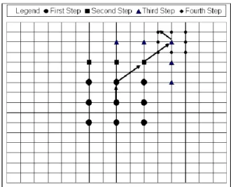
The main difference between 4SS and NTSS is the addition of Step 4. There is also an additional halfway-stop point in Step 2. An illustration of the 4SS search pattern taken from [9] is shown in Figure 2.4. In the first step there are 9 comparisons made. In the second step there could be 0, 3 or 5 comparisons. In the third step an additional 3 or 5 comparisons are made. In the final step 8 comparisons are made. Thus, the total number of comparisons is

n∈ {17,20,22,23,25,27}. (2.8) Thus, in the worst case, 4SS performs 5 fewer comparisons than NTSS. In [12] it is shown that the performance of 4SS is similar to NTSS in terms of MSE. A further extension of 4SS is Diamond Search (DS) [13], where the search window is in the shape of a diamond instead of a square. Additionally, the number of steps is not fixed and the procedure can carry on in the same manner after Step 4. It performs similarly to 4SS and performance can be improved by increasing the number of steps.

2.1.5 Adaptive Rood Pattern Search

The underlying assumption of Adaptive Rood Pattern Search (ARPS) [14] is based on the observation that the motion estimates become more precise

(22)

as one moves towards the global minimum of the error criterion. Thus, the authors make the assumption that the error surface is uni-modal. They also incorporate some correlation between motion vectors. Specifically, they assume that the horizontally adjacent blocks have similar motion vectors. For a certain block under consideration, the blocks in the direction of the motion vector of the left adjacent block are first searched before any further refinement. The procedure for ARPS is below:

1. Step 1: Compute the error between the current block and the corresponding block in the reference frame. If the error is less than some threshold T (T = 150 in [14]), then set the motion vector es-timate to (0,0) and end the procedure. Else, if the current block is the leftmost block in the search window set Γ = 2. Otherwise, Γ = max{|M V(x)|,|M V(y)|} where Γ is a measure of the maximum displacement of the left adjacent block and M V is the motion vector of the left adjacent block.

2. Step 2: Let the center of the current block be (x, y). Match the blocks at the positions (x±Γ, y ±Γ) and (x+M V(x), y +M V(y)). Find the point with the minimum error.

3. Step 3: Setup the window in the shape of the unit-size rood pattern and find the best match. Keep on iterating this procedure until the best match is found at the center of the search window.

2.2 Optical Flow

Optical flow methods relate changes between images by determining flow of intensities between images. Block matching algorithms are often counted as subsets of optical flow algorithms.Traditional optical flow algorithms often assume local smoothness and constant displacement flow to determine the displacement field. There are also methods which enforce global consistency of the field. In this section we will review standard optical flow methods and two recent methods based on deep neural networks.

(23)

2.2.1 Lucas-Kanade

The Lucas-Kanade (LK) method [15] is an optical flow algorithm developed in 1981. The method assumes that the displacement of a pixel between suc-cessive frames is small and constant within a small neighborhood around the point. Furthermore, the method assumes that the brightness remains unchanged between frames. These assumptions can be expressed mathemat-ically using the optical flow equations. Let the current pixel under consid-eration be (x, y, t) where t represent the current frame. Let the next frame occur in time ∆t. If the pixel moves in the direction (vx, vy) then according

to the brightness consistency equation

I(x, y, t) =I(x+vx, y+vy, t+ ∆t). (2.9)

Expanding the right-hand side of (2.9) using a first-order Taylor series ex-pansion we have: I(x, y, t) =I(x, y, t) + ∂I ∂xvx+ ∂I ∂yvy + ∂I ∂t∆t. (2.10)

From equation (2.10) we end up with the optical flow equation:

∂I ∂xvx+ ∂I ∂yvy =− ∂I ∂t∆t. (2.11)

To cope with the aperture problem, the Lucas-Kanade method solves for v

using local least-squares matching in a neighborhood around the pixel under consideration. Let the pixel under consideration be a and the neighborhood of points be P ={p1, . . . , pn}. The Lucas-Kanade method solves the

follow-ing minimization problem:

" vx vy # = argmin v1,v2 X p∈P (Ix(p)v1+Iy(p)v2+It∆t) 2 . (2.12)

A common variant of this method is to weight the pixels closer to a more than those farther away in the window. The minimization problem (2.12) is modified as: " vx vy # = argmin v1,v2 X p∈P wp(Ix(p)v1+Iy(p)v2+It∆t)2, (2.13)

(24)

where wp are the weights for each pixel. The optical flow equations can be

written in matrix form and can be solved using the normal equations.

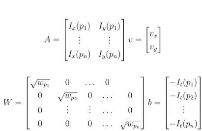
v = (A>W A)−1A>W b (2.14) A=     Ix(p1) Iy(p1) .. . ... Ix(pn) Iy(pn)     v = " vx vy # W =       √ wp1 0 . . . 0 0 √wp2 0 . . . 0 0 ... ... . . . 0 0 0 0 . . . √wpn       b =       −It(p1) −It(p2) .. . −It(pn)      

In this report we use a modern version of the Lucas-Kanade method available in Piotr’s Computer Vision Toolbox [16]. This version uses the weighted version of the Lucas-Kanade method and image pyramids. The algorithm uses a seven layer image pyramid with the highest level computing the flow on the image subsampled by 64 and refining the estimate in each level by warping the first image closer to the second. Best results were obtained by using a neighborhood of radius 10 pixels. The operation count on a 1024x640 image is shown in Table 2.1.

Table 2.1: Operation count for Lucas-Kanade to interpolate single frame of size 1024x640.

Layer Description Image Size Number of Multiply-Adds

Layer 1: Smoothen 16x10 3200

Layer 1: Matrix Calculations 16x10 82240

(25)

Layer 6: Matrix Calculations 512x320 8437760 Layer 7: Smoothen 1024x640 13107200 Layer 7: Matrix Calculations 1024x640 33751040

Total Operation Count 6.05×107

Number of ops/pixel 92

2.2.2 Horn-Schunck

The Horn-Schunck (HS) method [17], introduced in 1980, is a global method for optical flow estimation. Instead of assuming that the motion vectors remain constant locally around a point, the method optimizes for the flow by introducing a global smoothness parameter. The algorithm minimizes the distortion in the flow and the smoothness can be controlled by specifying the weight of a regularization parameter. The optical flow equation (2.11), and smoothness requirement are ensured through the minimization of the following energy function:

E = (Ixvx+Iyvy +It)2+α2(k∇vxk2+k∇vyk2), (2.15)

where the first term ensures brightness consistency and the second term ensures global smoothness. The above equation can be discretized for imple-mentation. The discretization is based on the central difference decomposi-tion of the Laplacian [18]. Details about the discretizadecomposi-tion can be found in [17]. Thus, the energy function can be approximated by:

E = (Ixvx+Iyvy+It)2+α2((vx−vx)2+ (vy −vy)2), (2.16)

wherevx andvy are a weighted average of the gradient from the surrounding

pixels. Taking the derivative with respect to vx and vy, we have

∂E ∂vx =−2α2(vx−vx) + 2(Ixvx+Iyvy+It)Ix, (2.17) ∂E ∂vy =−2α2(vy −vy) + 2(Ixvx+Iyvy+It)Iy. (2.18)

(26)

Solving the above two equations we get an expression for vx and vy which

can then be used to solve for the motion vectors.

(α2+I_x2+I_y2)(vx−vx) =−Ix(Ixvx+Iyvy +It), (2.19)

(α2+I_x2+I_y2)(vy −vy) =−Iy(Ixvx+Iyvy +It). (2.20)

The above equation tells us that the optimal motion vector should be close to the average of its surrounding motion vectors, i.e. the field is smooth. This will in-turn enforce brightness consistency. In practice, the motion vectors are solved for iteratively, by calculating the weighted average and then updating the vectors alternately.

v_xn+1 =vxn− Ix(Ixvxn+Iyvyn+It) (α2₊_I2 x +Iy2) , (2.21) v_yn+1 =vyn− Iy(Ixvxn+Iyvyn+It) (α2₊_I2 x +Iy2) . (2.22)

This algorithm is much more computationally intensive than the Lucas-Kanade method. The execution time depends on the smoothness of the image and the number of iterations required for convergence.

2.2.3 Black and Anandan

Black and Anandan introduced the idea of robust penalization for optical flow estimation in their paper in 1991 [19]. Until 1991, most optical flow algorithms, such as LK and HS, used the `2 norm (least squares) as the cost

function or penalization function. The growth rate of the `2 norm is faster

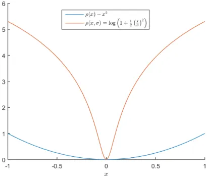
and it tends to not penalize erroneous estimates much more than accurate estimates. Black and Anandan proposed the use of a cost function that strongly penalizes large errors while rewarding accurate estimates. In par-ticular, the cost function for LK and HS can be modified as shown in (2.23) and (2.24) respectively. ELK = X p∈P ρ(Ix(p)v1+Iy(p)v2+It∆t, σ) (2.23) EHS =λDρD(Ixvx+Iyvy +It, σD) +α2(ρS(vx−vx, σS) +ρS(vy−vy, σS)). (2.24)

(27)

Figure 2.5: Lorentzian norm and `2 norm.

Here ρD, ρS are the robust norms and σD, σS are control parameters. Black

and Anandan use the Lorentzian error norm for bothρD andρS. Notice how

it penalizes large errors in Figure 2.5.

The motion vectors can be solved for by minimizing the above cost functions using gradient descent. The derivatives of the cost function can be calculated the same way as in the LK or HS method. A detailed derivation of the gradient descent formulas can be found in [19]. The final equations are:

v_x(n+1) =v_x(n)−ω 1 T(x, y) ∂E ∂vx , (2.25) v_y(n+1) =v_y(n)−ω 1 T(x, y) ∂E ∂vy . (2.26)

HereT(x, y) is a bound on the second derivative of the cost function andωis the step-size of the update. The Black and Anandan method heralded the use of robust penalization cost functions for optical flow estimation. Such cost functions are still used in many modern deep learning optical flow algorithms, the most popular error metric being the `1 norm.

(28)

2.2.4 MDP-Flow2 and Deepflow2

There are many more optical flow algorithms that can be discussed. Optical flow estimation is one of the most challenging computer vision problems to date and a thorough discussion of all algorithms would require many more pages. Further literature on optical flow can be found in [20, 21, 22]. It is worth mentioning two recent approaches to optical flow based on feature matching and neural networks.

Motion Detail Preserving Flow v2 (MDP-Flow2) [23] is currently one of the top ranked flow algorithms on the Middlebury flow rankings and it held the top spot for some time in 2010. The algorithm uses an image pyramid to predict flow on different levels (i.e. different amplitudes). In each level, the flow is computed by performing feature matching across the whole image and patch matching using 16×16 blocks. Following this, multiple flow candidates are generated to account for occlusions. A simple least squares optimization provides the best candidate. The flow is then made continuous by minimizing the Total Variation (TV) energy function. The image is then warped closer to the true version using the flow estimates and the estimates are continued on to the next level.

Deepflow 2 [24] performs a similar feature matching algorithm as in MDP-Flow2. The matching algorithm is called Deepmatching. It uses a pyramid structure with data movement interleaved between the levels, akin to the structure of a convolutional neural network. The cost function minimized is a robust penalizer and it is nearly the same as the BA cost function with an additional matching energy introduced from the Deepmatching algorithm. Deepflow2 is also ranked as one of the top optical flow methods on the Mid-dlebury dataset.

An in-depth analysis of the algorithms can be found in the papers cited previously. Details have been left out as the analysis of these algorithms is not the goal of this thesis. It should be noted that the above algorithms have been specially optimized for the Middlebury dataset and are computationally expensive.

(29)

CHAPTER 3 FRAME INTERPOLATION

Frame interpolation refers to generating a new image given an observed input sequence. In MCFI, interpolation is performed by using the displacement field obtained by the motion estimation algorithm. In most applications, frame interpolation is performed by using only two reference frames. Better interpolation results can be obtained by using multiple images of the same scene. In such cases, the images can be mapped to the same frame of reference by using image registration techniques [25].

3.1 MCFI Problem Statement

In this thesis we will focus on frame interpolation with the only priors being two input frames. Let the input frames be It and It+1. Let u be the

dis-placement field after performing motion compensation. The goal of MCFI is to generate an intermediate frame It+1/2 such that

It+1/2(x) = It(x−u/2), (3.1)

It+1/2(x) = It+1(x+u/2). (3.2)

The generation of this intermediate frame using the motion vectors is the task of frame interpolation. In the next few subsections we will review some common interpolation techniques. Finally, we will look at a recently devel-oped CNN approach for video frame interpolation that estimates separable interpolation kernels.

(30)

3.2 Interpolation Algorithms

We will review five different image interpolation algorithms in this section. While images are defined on a discrete grid, we will assume that the grid is continuous to simplify the theory. Furthermore, we will assume that the points in the input image are spaced at a distance of 1 unit apart in the vertical and horizontal directions.

Image averaging is the only technique that requires two input images. All other interpolation techniques discussed in this section require a single input image.

3.2.1 Image Averaging

Image averaging is the simplest form of interpolation that one can perform between two images. The interpolated image Iint can be expressed in terms

of the input images I1 and I2 as:

Iint(x, y) =

I1(x, y) +I2(x, y)

2 . (3.3)

This interpolation is sufficient to use when there is very minimal or no motion between frames. This method tends to blend colors and creates artificial looking images with many artifacts.

3.2.2 Nearest Neighbor Interpolation

Nearest neighbor assigns the interpolated point with the value of its closest neighbor in the input image. For a 1D signal this can be carried out through convolution with the following kernel:

ϕ(x) =          0 x <−1 2 1 −1 2 ≤x≤ 1 2 0 x > 1₂ . (3.4)

For a 2D signal, this kernel is applied in the horizontal and vertical direction in a separable fashion.

(31)

3.2.3 Bandlimited vs. Spline Interpolation

In traditional interpolation, a function f is approximated using the samples

fn = f(nT), and a set of interpolation basis functions {ϕint _Tx −k

}k∈Z. The basis function satisfies ϕint(n) = δn, n ∈ Z, where δn is the Kronecker

delta function. The approximated function can be constructed as follows:

fint(x) = X k∈_Z fkϕint x T −k . (3.5)

In the case of signals bandlimited to

−π T,

π T

, we can makefint=f by using

ϕint = sinc. The sampling property and infinite support of the basis

func-tions result in these funcfunc-tions being impractical to use in practice.

In generalized interpolation, the goal is to still approximate a function as closely as possible. However, the interpolation basis functions are no longer required to satisfy the sampling property. Furthermore, for computational purposes, basis functions with finite support are chosen. One particular example of such an interpolation basis function is a spline which is discussed in more detail in Section 3.2.4. (3.5) is modified as shown below:

fint(x) = X k∈_Z ckϕ x T −k . (3.6)

Notice that the coefficients in (3.6) are no longer the sample values of the function. Thus, we need an additional constraint. We should require that the sample values at integer multiples of T can be reconstructed. Thus,

fn=f(nT) = X

k∈_Z

ckϕ(n−k) = (c∗ϕ)n. (3.7)

In the z-domain, this relationship can be expressed as a filtering operation.

C(z) = _P 1

n∈_Zϕ(n)z−n

F(z), (3.8)

whereF(z) is the z-transform of the samples off. As long asP

n∈Zϕ(n)z

−n

has no roots on the unit circle, the above filtering operation can be imple-mented as forward-backward filtering operation using the causal and anti-causal parts of the basis function.

(32)

Thus, generalized interpolation can be split into two steps: 1. Determine the coefficients cn using (3.8).

2. Perform interpolation using (3.6).

Generalized interpolation is often used because we have the choice of us-ing a larger range of interpolation basis functions based on the application and system constraints. An important metric for assessing an interpolant’s quality is know as the approximation order. An interpolant with degree of approximation L satisfies the following relation:

kf−fintk2 ≤C×TL. (3.9)

Here, C is called the approximation gain and T is the time step used in sampling f.

3.2.4 Splines

Splines are smooth piecewise polynomials. A spline with degree K has con-tinuous derivatives up to order K−1 and it is differentiable up to order K

everywhere except at the piece boundaries. Since splines are piecewise, the expression of the polynomials that compose the spline change at different points. These points are calledknots. We will only consider uniform splines, where the knots are evenly spaced out.

The most commonly used spline basis functions are the elementary B-splines. The elementary B-spline of degree 0 is given by:

β(0)(x) =    1 −1 2 ≤x < 1 2 0 otherwise . (3.10)

There are slight differences between the elementary B-spline of degree 0 and the nearest neighbor interpolation kernel; particularly, the spline averages values at half-integer points while the latter kernel does not [26]. The B-splines of higher degree can be derived from the elementary B-spline of degree

(33)

Figure 3.1: Illustration of different interpolation techniques. 0 by the following recursive formula:

β(n)(x) = β(n−1)∗β(0)(x). (3.11) Splines of degreenhave an approximation order ofn+1. This means that the function is very smooth. Splines also have the property of having the highest approximation order for a given support. A thorough review of splines can be found in [27]. Figure 3.1 [28] shows common interpolation techniques employed in image processing.

3.2.4.1 Linear Interpolation

Linear interpolation is performed by using the elementary B-spline of degree 1. β(1)(x) =          1 +x 1≤x <0 1−x 0≤x <1 0 otherwise . (3.12)

Notice that the range of the kernel is 2 units. In an image this would utilize up to three pixels in both the horizontal and vertical direction to compute the interpolated pixel. Interpolation is first carried out in the horizontal di-rection followed by interpolation in the vertical didi-rection. This is commonly known as bilinear interpolation.

The coefficientscncan be determined by solving (3.8). For an image we need

to first evaluate ϕ=β(1) _{at all integer points in the basis function’s support.}

(34)

x -4 -3 -2 -1 0 1 2 3 4 0 0.1 0.2 0.3 0.4 0.5 0.6 0.7 0.8 0.9 1 β(3)₍x) β(1)(x)

Figure 3.2: Linear and cubic elementary B-splines. the inverse z-transform of C(z).

C(z) = 1

1 + 2(z+ 1/z)F(z), (3.13) The above filtering operation can be expressed as a forward-backward filter-ing operation by observfilter-ing that 1 + 2(z+ 1/z) = _λ12(1−λz

−1₎₍₁₋_λz_{) where}

λ = 1₄i(√15 +i).

3.2.4.2 Cubic Interpolation

Cubic interpolation is performed by using the elementary B-spline of degree 3. β(3)(x) =          2 3 − 1 2|x| 2₍₂_{− |}_x_|) ₀_{≤ |}_x_|_<₁ 1 6(2− |x|) 3 ₁_{≤ |}_x_|_<₂ 0 otherwise . (3.14)

Notice that the range of the kernel is 4 units. In an image this would utilize up to five pixels in both the horizontal and vertical direction to compute the interpolated pixel. Figure 3.2 illustrates the difference between the elemen-tary linear and cubic spline kernels. Interpolation is first carried out in the horizontal direction followed by interpolation in the vertical direction. This is commonly known as bicubic interpolation.

(35)

x -4 -3 -2 -1 0 1 2 3 4 0 0.1 0.2 0.3 0.4 0.5 0.6 0.7 β(3)₍x) ϕ(3)(x)

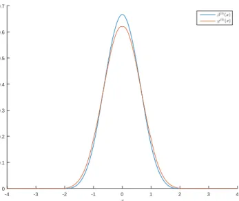
Figure 3.3: Cubic B-spline and OMOMS comparison.

The coefficientscncan be determined by solving (3.8). For an image we need

to first evaluate ϕ=β(3) _{at all integer points in the basis function’s support.}

Thus,ϕn = 1₆δn+1+₃2δn+1₆δn−1. The coefficients can now be found by taking

the inverse z-transform of C(z) as was detailed in Section 3.2.4.1.

3.2.5 Cubic-OMOMS

Cubic splines fall under the category of interpolating functions known as Maximal-Order Interpolation of Minimal Support (MOMS) [29]. These are the class of functions that have the highest degree of approximation for a given support. The class of interpolants knows as Optimal Maximal-Order Interpolation of Minimal Support (OMOMS) [29] are those MOMS functions with the smallest approximation gain, C, in the `2 _{sense. These OMOMS}

functions can be expressed in terms of the elementary B-spline functions and its derivatives. The formula for the cubic-OMOMS interpolant is:

ϕ(3)_o (x) = β(3)(x) + 1 42 d2 dx2β (3) (x) (3.15) ϕ(3)_o (x) =          1 2|x| 3 _{− |}_x_|2₊ 1 14|x|+ 13 21 0≤ |x|<1 −1 6|x| 3₊_|_x_|2₋ 85 42|x|+ 29 21 1≤ |x|<2 0 otherwise . (3.16)

(36)

The coefficient C is 4.6 times smaller for OMOMS in comparison to the similar coefficient for cubic splines. Figure 3.3 illustrates the difference in scaling between the elementary cubic spline and the cubic-OMOMS kernel. OMOMS have shown to produce slightly better interpolation results than MOMS functions [29].

3.3 Adaptive Separable Convolution

Instead of using optical flow estimates to perform frame interpolation, Niklaus et al. [30] use a deep convolutional neural network (CNN) to estimate sep-arable convolution kernels that can be used to determine the intensity of each pixel in the output image. This method is known as adaptive separable convolution.

3.3.1 Problem Statement

The goal is to interpolate a frame Iint between two input frames I1 and I2.

For each output pixel (x, y) in Iint, the CNN estimates a pair of separable

filters K1 and K2 such that

Iint(x, y) =K1(x, y)∗P1(x, y) +K2(x, y)∗P2(x, y), (3.17)

where P1 and P2 are patches of the images centered around the pixel (x, y)

in the images I1 andI2 respectively. The separable filters can be represented

as hK1v, K1hi and hK2v, K2hi. Then,

Ki =Kiv×Kih>, i= 1,2 (3.18)

Niklaus et al. use kernels of size 51×51. Thus, a total of 204 floating point values need to be stored per pixel. For a 1080p image, this would require 204×1920×1080 = 1.58 GB memory.

(37)

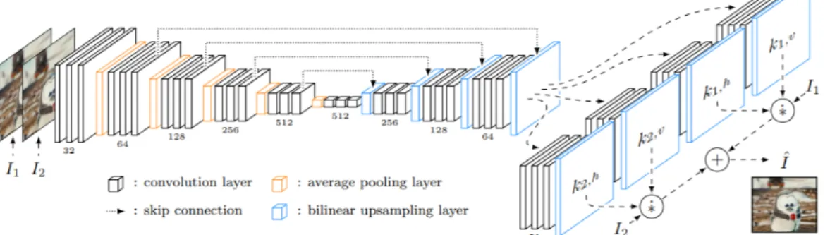
Figure 3.4: Illustration of neural network architecture. Given input frames

I1 and I2, an encoder-decoder network extracts features that are given to

four sub-networks that each estimate one of the four 1D kernels for each output pixel in a dense pixel-wise manner. The estimated pixel-dependent kernels are then convolved with the input frames to produce the

interpolated frame Iint.

3.3.2 Network Architecture

The network has a contracting section followed by an expanding section as is shown in Figure 3.4 (The figure was taken from [30]). The layers are organized as a sequence of three convolutional layers followed by a ReLU activation layer. Skip connections are present between the contracting and expanding parts to facilitate the sharing of information before the downsam-pling operation and to improve the stability of the network at the upsamdownsam-pling layers. The authors use bilinear interpolation in the upsampling layers. The authors trained the model with two loss functions. The first one is the L1 norm.

L1 =kIint−Igtk1 (3.19)

They also trained it with a perceptual loss function (LF). Perceptual loss

is based on certain high level features that the user chooses to extract from the images. The relu4 4 layer from the VGG19 network was used for the aforementioned purpose.

LF =kφ(Iint)−φ(Igt)k22 (3.20)

The authors trained the network for 20 hours on an NVIDIA Titan X (Pas-cal) GPU. A detailed breakdown of the various layers and operation count is

(38)

given in Table 3.1. The authors trained it on patches of images taken from common YouTube videos using AdaMax.

The operation count was separated into multiply-additions and in-place com-putations to ease the counting process. The authors implemented the last two layers in CUDA to perform fast computations.

Table 3.1: Operation count for Adaptive Separable Convolution to interpolate single frame of size 960×540×3.

Layer Output Size Multiply-Adds Add, Div etc.

Input (1024, 640, 6) 0 0 Conv + ReLU (1024, 640, 32) 1132462080 20971520 Conv + ReLU (1024, 640, 32) 6039797760 20971520 Conv + ReLU (1024, 640, 32) 6039797760 20971520 Avg. Pool (512, 320, 32) 0 20971520 Conv + ReLU (512, 320, 64) 3019898880 10485760 Conv + ReLU (512, 320, 64) 6039797760 10485760 Conv + ReLU (512, 320, 64) 6039797760 10485760 Avg. Pool (256, 160, 64) 0 10485760 Conv + ReLU (256, 160, 128) 3019898880 5242880 Conv + ReLU (256, 160, 128) 6039797760 5242880 Conv + ReLU (256, 160, 128) 6039797760 5242880 Avg. Pool (128, 80, 128) 0 5242880 Conv + ReLU (128, 80, 256) 3019898880 2621440 Conv + ReLU (128, 80, 256) 6039797760 2621440 Conv + ReLU (128, 80, 256) 6039797760 2621440 Avg. Pool (64, 40, 256) 0 2621440 Conv + ReLU (64, 40, 512) 3019898880 1310720 Conv + ReLU (64, 40, 512) 6039797760 1310720 Conv + ReLU (64, 40, 512) 6039797760 1310720 Avg. Pool (32, 20, 512) 0 1310720 Conv + ReLU (32, 20, 512) 1509949440 327680 Conv + ReLU (32, 20, 512) 6039797760 327680 Conv + ReLU (32, 20, 512) 6039797760 327680 Upsample Bilinear (64, 40, 512) 11796480 0 Conv + ReLU (64, 40, 512) 6039797760 1310720

(39)

Conv + ReLU (64, 40, 256) 3019898880 655360 Conv + ReLU (64, 40, 256) 1509949440 655360 Conv + ReLU (64, 40, 256) 1509949440 655360 Upsample Bilinear (128, 80, 256) 23592960 0 Conv + ReLU (128, 80, 256) 6039797760 2621440 Conv + ReLU (128, 80, 128) 3019898880 1310720 Conv + ReLU (128, 80, 128) 1509949440 1310720 Conv + ReLU (128, 80, 128) 1509949440 1310720 Upsample Bilinear (256, 160, 128) 47186920 0 Conv + ReLU (256, 160, 128) 6039797760 5242880 Conv + ReLU (256, 160, 64) 3019898880 2621440 Conv + ReLU (256, 160, 64) 1509949440 2621440 Conv + ReLU (256, 160, 64) 1509949440 2621440 Upsample Bilinear (512, 320, 64) 94371840 0 Conv + ReLU (512, 320, 64) 6039797760 10485760 Separable Filters (1024, 640, 51) 1011 108 Output (1024, 640, 3) 2.5×1011 0

(40)

CHAPTER 4 LOCAL ALL-PASS FILTERS

Most traditional optical flow algorithms estimate the optical flow using the optical flow equation defined in (2.11). They either enforce this constraint by assuming a locally constant flow and thus a small displacement field (e.g. LK) or by enforcing global consistency (e.g. HS). However, even in many cases when the optical flow field is smooth, the displacement amplitude between two images might not be small. Gilliam et al. solve this problem by relating local changes through an all-pass filtering framework known as the Local All-Pass algorithm (LAP) [31, 32, 33, 34]. In the rest of this chapter we will summarize the LAP algorithm detailed in [34].

4.1 Main Principles of the LAP Framework

The All-Pass filter framework is built upon five guiding principles which are detailed below.

4.1.1 Shifting is All-Pass Filtering

If the brightness consistency holds, shifting an image in the time domain in the direction of a constant displacementu(x, y) = (u1, u2)> can be expressed

in the frequency domain as ˆ

I2(ω1, ω2) = ˆI1(ω1, ω2)e−jω1u1−jω2u2, (4.1)

where ˆI is the Fourier transform ofI. The previous expression can be inter-preted as filtering I1 with a filterh having frequency response

ˆ

(41)

This is a filter that is separable, real valued and all-pass i.e. |ˆh(ω1, ω2)|= 1.

Notice that the flow displacement information is contained within the phase of this filter. Thus, once this filter is estimated, the optical flow can be ex-tracted through simple differentiation operations. While the filter discussed above is continuous, the same properties hold in the discrete domain under ideal sampling of h with the sinc kernel.

4.1.2 Rational Representation of All-Pass Filter

Any real all-pass filter can be expressed as the ratio of two real digital filters with the same amplitude and opposite phase. If the desired phase of the all-pass filter ˆh(ω1, ω2) is 2arg(ˆp(ω1, ω2)), then

ˆ h(ω1, ω2) = ˆ p(ω1, ω2) ˆ p(−ω1,−ω2) , (4.3)

where ˆp(ω1, ω2) is the forward filter and ˆp(−ω1,−ω2) is the backward filter.

Now (4.1) can be rewritten as ˆ I2(ω1, ω2) = ˆI1(ω1, ω2) ˆ p(ω1, ω2) ˆ p(−ω1,−ω2) (4.4) In the time domain this can be expressed as a forward-backward filtering relation:

I2[k, l]∗p[−k,−l]−I1[k, l]∗p[k, l] = 0, (4.5)

where (k, l) are discrete pixel coordinates. Thus, estimatingh boils down to estimating p.

4.1.3 Linear Approximation of Forward Filter

Gilliam and Blu [31, 34] use a standard signal processing technique to approx-imate the forward filterpusing a set of fixed real filterpn. The approximation

can be expressed as:

papp[k] = N−1 X

n=0

(42)

where k = (k, l)>. Estimating p now only involves finding the appropriate coefficients cn. This can be done via a simple least squares minimization

procedure which will be discussed later. The authors also note that while the separability of the all-pass filter is lost, the filter is still real.

4.1.4 Choosing a Good Filter Basis

The filter basis was chosen keeping two important points in mind:

1. The number of filters N must be much smaller than the number of pixels in the image.

2. The number of filters N should be independent of the priori assump-tions of the displacement amplitudeR. In other words, the filter should be able to scale easily to estimate different displacements.

A naive choice for the filter basis would be canonical representation of finite impulse response filters (FIR) over the range [−R, R], i.e. the square of side 2R+ 1:

ˆ

pn =e−jω1kn−jω2ln, (4.7)

wherekn, ln∈[−R, R]. This is not a good choice since estimating a

displace-ment of R would require N =O(R2) basis filters.

After experimenting with different empirical methods, Gilliam and Blu ob-served that the forward filters approximated from these methods were closely related to a Guassian filter and its derivatives. The basis filters are divided into two categories: 1) K = 1 (Gaussian filter and first derivatives) which results inN = 3 filters or 2) K = 2 (Gaussiam filter and first, second deriva-tives) which results in N = 6 filters. This filter basis is shown in (4.8).

K = 1 includes pi[k], i = 0,1,2 and K = 2 includes pi[k], i = 0,1,2,3,4,5.

(43)

filter. Notice that these filters can be easily scaled for large displacements. K = 1            p0[k] = exp −k 2₊_l2 2σ2 p1[k] =kp0[k] p2[k] =lp0[k] p3[k] = (k2+l2−2σ2)p0[k] p4[k] =klp0[k] p5[k] = (k2−l2)p0[k]                              K = 2 (4.8)

The theoretical properties of these filters and the approximation order of the filter basis are detailed in [33]. Using Pad´e approximations it was shown that the approximation order of the filter basis is L = 2K. Thus, in the case of

K = 1 the approximation order is 2 and forK = 2 the approximation order is 4. This is a promising result because most state-of-the-art optical flow methods have an approximation order of 1.

4.1.5 Displacement Vector from All-Pass Filter

Since the all-pass filter happis expected to be close to (4.2), the displacement

vectors can be extracted from the frequency response of the filter as:

u1,2 =j ∂log(ˆhapp(ω1, ω2)) ∂ω1,2 _ω 1=ω2=0 . (4.9)

Using the rational representation of the all-pass filter, the displacement vec-tors can be found using a simple formula in terms of the impulse response of the forward filter:

u1 = 2 P kkp[k] P kp[k] and u2 = 2 P klp[k] P kp[k] , (4.10)

where the summation is over all discrete points in the region of support of the signal.

(44)

(a)I1 (b)I2 (c) Ground Truth

(d) LAP (e) Lucas-Kanade (f) Horn-Schunck

Figure 4.1: Estimated flow using different methods. A radius of 10 was used for LK and HS. HS required 250 iterations for convergence. LAP flow was estimated using all six basis filters.

4.2 Estimation of All-Pass Filter

The estimation of the all-pass filter is performed by adapting (4.5) locally around every pixel in a window, W, of size 2W + 1 × 2W + 1. In the implementation of the algorithm W = R except when R < 1. Gilliam and Blu coin a new relation known as local all-pass equation defined as follows:

papp[k]∗I1[k] =papp[−k]∗I2[k], k ∈ W, (4.11)

where papp[k] is given in (4.6).

To enforce the local all-pass equation, the difference between the left and right side in (4.11) can be minimized in the `2 sense. Defining hJiW =P_k∈WJ[k] and p_app[k] =papp[−k], the minimization problem can be written as:

min {cn} h(papp∗I1−papp∗I2)2iW, (4.12) where papp[k] =p0[k] + N−1 X n=1 cnpn[k].

(45)

fol-lowing equations in cn: 0 =h(pn∗I1−pn∗I2)(p0∗I1−p0∗I2)iW (4.13) + N−1 X n0₌₁ cn0h(p_n∗I₁−p_n∗I₂)(p_n0 ∗I₁ −p_n0 ∗I₂)iW for n = 0,1, . . . , N −1.

The previous equations can be solved very efficiently using pointwise multipli-cations and fast convolutions. Gilliam and Blu solve the system of equations using Gaussian elimination which has a constant number of operations per each pixel.

4.3 Poly-Filter Extension

The LAP algorithm is able to estimate large displacements, but it requires a filter basis with large support. To estimate smoothly varying flows, iterative refinement is performed to estimate the flow at various levels i.e., flows with varying amplitude. Instead of using image pyramids, Gilliam and Blue use filter pyramids. In each iteration of the algorithm, the support of the filter is changed. Thus, the only parameter that changes is R. This extension is termed as Poly-Filter LAP (PF-LAP). The LAP and PF-LAP algorithms from [34] have been reproduced as Algorithm 1 and 2 respectively in this thesis for sake of completion.

PF-LAP is implemented as follows: The user can choose the maximum sup-port Rmax. Create the filter basis for this support and estimate the

de-formation field using the LAP algorithm. Warp I2 closer to I1 using this

deformation field. Perform post-processing on this deformation field to re-move NaNs and to smoothen the field. In the next iteration decrease the support width by a factor of 2 and repeat the procedure again. This process continues until R= 1. Finally, one more iteration is performed with R= 0.5 to accurately estimate any subpixel flows. The operation count for the LAP algorithm to interpolate a frame of size 960x540x3 is shown in Table 4.1.

(46)

Algorithm 1 Local All-Pass (LAP estimation of a deformation field)

Inputs: Images I1 and I2, filter size R and number of filters N

1: Initialization: Generate the filter basis in (4.8) using R and N.

2: Filter Estimation: Using the filter basis, solve the minimization problem by using (4.13) to obtain the filter coefficients.

3: Extraction: Using the filter coefficients obtain the approximate forward filter. Use (4.10) to solve for the displacement field.

Algorithm 2 Poly-Filter Local All-Pass algorithm

Inputs: Images I1 and I2, number of levels R and number of filters N

1: Initialization: Set u2R+1 =0 and I₂shift =I₂.

2: for R in [2R_{, 2}R−1_{, . . . , 0.5]} _do

3: Pre-Filtering (OPTIONAL): Construct filter p0 from (4.8) and obtain

high-pass images I₁hp and I₂hp.

4: Estimation: Using N and R estimate the deformation increment ∆u

between the imagesI1 and I2 (or high-pass images if R <1) using the

LAP algorithm defined in Algorithm 1.

5: Post-Processing: Using inpainting procedure and median filtering to remove erroneous estimate. Then smooth the flow using a Gaussian filter.

6: Update: SetuR =u2R+ ∆u

7: Warping: Warp I2 closer to I1 using uR to obtain I2shift. If R ≤ 2 use

cubic-OMOMS interpolation else use shifted-linear interpolation.

8: end for

4.4 Pre-Processing and Post-Processing Tools

In PF-LAP, image pre-processing is performed to reduce the effect of slowly varying illumination changes at very course levels. Specifically, during sub-pixel flow estimation the high-pass filtered images are used. This is done by low pass filtering the images using p0 and subtracting this from the original

image:

I_ihp=Ii−p0∗Ii. (4.14)

At the end of each iteration in PF-LAP, I2 is warped towards I1 using the

estimated field. High-quality interpolation is achieved using cubic splines or cubic-OMOMS (see Sections 3.2.4.2 and 3.2.5). To ensure fast interpolation, shifted-linear interpolation (see Section 3.2.4.1) is performed for R > 2 and cubic-OMOMS is used for R ≤ 2. To remove erroneous estimates a round

(47)

of median filtering and simple convolutional image inpainting is performed on the displacement field. Finally, the flow is smoothened using a Gaussian filter with variance half the support.

In the remainder of the thesis we will refer to PF-LAP as LAP to refer to the overall algorithm.

Table 4.1: Operation count for LAP to interpolate a single frame of size 960x540x3. Below, ma stands for multiply-adds and the cleaning

procedures involve NaN inpainting, mean and median filtering. Flow estimation requires 3 subtractions, 2 divisions and 1 addition per pixel.

Function No. of Ops

Image pre-filtering with high-pass filter (3x3x3) 13996800 Level 1 Basis filtering (17x17x3) 1348358400 Level 1 Gaussian Elimination (5 ma) 7776000

Level 1 Flow estimate 3110400

Level 1 Cleaning Procedures 9331200

Level 1 Shifted Linear Interpolation (2 significant ma) 3110400

Level 2 Basis filtering (9x9x3) 377913600

Level 2 Gaussian Elimination (5 ma) 7776000

Level 4 Cubic Interpolation (6 significant ma) 77760000

(48)

CHAPTER 5 VIDEO INTERPOLATION RESULTS

In this chapter we quantitatively and qualitatively assess the video interpola-tion quality obtained using three methods: LAP (Chapter 4), Lucas-Kanade (Section 2.2.1) and Adaptive Separable Convolution (Section 3.3). To ease notation we will refer to Lucas-Kanade as LK and Adaptive Separable as CNN (since it is based on a CNN). Note that the K = 1 version of the LAP algorithm is used (Section 4.3).

We perform video interpolation on Derf’s Media Collection [35] and the EPIC Kitchen’s dataset [36]. Both these datasets contain sequences captured at a temporal resolution of 60 frames per second which is ideal for studying interpolation. We also perform interpolation experiments on the Middlebury dataset [22], a standard dataset used for benchmarking a variety of image processing algorithms. MDP-Flow2 and Deepflow2 (Section 2.2.4) interpo-lation is also performed to assess the quality of the top performers on the Middlebury benchmark.

Finally, we will comment on the correlation between quantitative metrics and qualitative metrics by conducting a user study on a sample of the video sequences.

All experiments were performed on an Intel Core i7-8750H processor with 32 GB RAM. The CNN was executed on an NVIDIA GTX 1050Ti GPU with 4GB RAM. The interpolation results can be viewed athttps://bit.ly/2WqXbKR. Sequences should be downloaded else the media player will drop the inter-mediate frames!

(49)

Table 5.1: MSE evaluation on the Middlebury dataset (high-speed camera samples). Bold values indicate best results.

Beanbags DogDance MiniCooper Walking Backyard Basketball Dumptruck Evergreen LAP 339.0 240.1 176.7 67.9 163.5 198.9 209.3 268.6

CNN 196.9 159.4 80.5 57.2 102.6 105.8 88.3 102.8

LK 454.7 223.9 233.2 97.3 273.5 157.2 281.7 276.8

5.1 Performance Evaluation Criteria

In addition to computational speed, it is desirable to employ an objective per-formance metric to evaluate the match between the interpolated frame and the ground truth. The standard criterion is the ubiquitous Mean-Squared Error (MSE) [6]. Unfortunately MSE is a particularly bad criterion for mea-suring the quality of interpolated images, as slight misalignments can be quite acceptable perceptually yet cause large squared errors [37]. We have experimented with other metrics such as SSIM [38] and CW-SSIM [39] but they suffer from similar artifacts. Therefore we rely extensively on visual evaluation to assess performance of competing algorithms. The discrepancy between MSE and perceptual quality is often striking.

5.2 Middlebury Dataset

MSE results for the Middlebury dataset are given in Table 5.1. Although the CNN seems to perform the best interpolation in terms of MSE, we ob-serve that actually the LAP consistently interpolates frames with the highest perceptual quality. This is evident from Figure 5.1: Notice how the palms are smudged and how the balls are distorted in the CNN interpolated frame. Yet, since the imprints of the middle two balls are slightly closer to the actual position of the balls, the CNN interpolated frame has a lower MSE. There is also a greater intensity match between the pixels in the original image and the CNN-interpolated image in comparison to the LAP-interpolated images. The Lucas-Kanade method performed poorly on all sequences. The flow field across the juggler’s torso is incorrect. The fingers are deformed in Figure 5.1, and the blinds are skewed due to inexact optical flow estimates. This is evi-dent from the patch of blue on the door in the zoomed in image of the balls.

(50)

First frame Second frame Third frame

(a) Original (b) LAP (c) CNN (d) LK

Figure 5.1: Beanbags sequence: The original sequence is shown at the top. The original second frame is shown in (a), the LAP-interpolated second frame is shown in (b), the CNN-interpolated second frame is shown in (c), the LK-interpolated second frame is shown in (d). LAP was used to compute the optical flow in (a), (b) and (c).

(51)

Table 5.2: Average interpolation MSE on Derf’s Media Collection. Bold

values indicate best results.

LAP CNN LK city 62.1 79.8 111.7 crew 522.1 406.1 806.5 harbour 112.2 94.8 117.1 ice 129.6 57.4 109.9 soccer 848.3 141.6 399.5 stockholm 54.6 60.4 77.6 riverbed 361.7 409.6 445.8

Also notice how the left side of the juggler’s torso has been warped inwards. The displacement field for the LAP algorithm is the closest to the flow between the original frames. The optical flow between the original frame and CNN-interpolated frame is not as smooth in the blue-yellow region boundary in comparison to the flow between the original frame and LAP-interpolated frame. This results in the juggler’s palms being blurred in the CNN-interpolated frame.

5.3 Derf’s Media Collection

This dataset consists of video sequences which are generally used to evaluate compression algorithms. Table 5.2 shows the interpolation results on seven 60 fps videos with 704x576 spatial resolution. We dropped every other frame in the video sequence and interpolated between the remaining pairs.

Table 5.2 shows MSE results, and Fig. 5.2 shows frames for the soccer se-quence. While the LAP method yields good visual quality, a visible artifact is the position of the running player in the LAP-interpolated frame, which is slightly to the left of his position in the original frame. The player’s leg is also slightly lower and farther away from his body in comparison to the original frame. Still, when viewed as a sequence, the LAP-interpolated video looked natural and smooth.

(52)

Frame 313 Frame 314 Frame 315

(a) Original (b) LAP (c) CNN (d) LK

Figure 5.2: Soccer sequence: The original sequence is shown at the top. Original frame 314 is shown in (a), LAP-interpolated frame 314 is shown in (b), CNN-interpolated frame 314 is shown in (c) and the LK interpolated 314 is shown in (d). The optical flow between frame 314 and frame 314 is shown for the original sequence in (a) and for the three methods in the other columns. LAP was used to compute the optical flow in (a), (b) and (c).

The Lucas-Kanade method did not compute a very precise flow field. Notice how the displacement vectors are pointing south across the running player. This results in the fence being highly deformed in the interpolated frames. When the interpolated frames are played at 60 frames per second, this causes flickering and strenuous visual artifacts. The neural network almost aligns

LAP-based motion-compensated frame interpolation

ABSTRACT

ACKNOWLEDGMENTS

TABLE OF CONTENTS

LIST OF TABLES

LIST OF FIGURES

LIST OF ABBREVIATIONS

CHAPTER 1

INTRODUCTION

1.1

Background

1.1.1

Motion-Compensated Frame Interpolation

1.2

Thesis Objectives

1.3

Organization of Thesis

CHAPTER 2

MOTION ESTIMATION

2.1

Block Matching

2.1.1

Full Search

2.1.2

Three-Step Search

2.1.3

New Three-Step Search

2.1.4

Four-Step Search

2.1.5

Adaptive Rood Pattern Search

2.2

Optical Flow

2.2.1

Lucas-Kanade

2.2.2

Horn-Schunck

2.2.3

Black and Anandan

2.2.4

MDP-Flow2 and Deepflow2

CHAPTER 3

FRAME INTERPOLATION

3.1

MCFI Problem Statement

3.2

Interpolation Algorithms

3.2.1

Image Averaging

3.2.2

Nearest Neighbor Interpolation

3.2.3

Bandlimited vs. Spline Interpolation

3.2.4

Splines

3.2.5

Cubic-OMOMS

3.3

Adaptive Separable Convolution

3.3.1

Problem Statement

3.3.2

Network Architecture

CHAPTER 4

LOCAL ALL-PASS FILTERS

4.1

Main Principles of the LAP Framework

4.1.1

Shifting is All-Pass Filtering

4.1.2

Rational Representation of All-Pass Filter

4.1.3

Linear Approximation of Forward Filter

4.1.4

Choosing a Good Filter Basis

4.1.5

Displacement Vector from All-Pass Filter

4.2

Estimation of All-Pass Filter

4.3