with Kernel Embeddings
Mijung Park∗ † Wittawat Jitkrittum∗ Dino Sejdinovic
[email protected] Gatsby Unit University College London
[email protected] Gatsby Unit
University College London
[email protected] Department of Statistics
University of Oxford
Abstract
Complicated generative models often result in a situation where computing the likelihood of observed data is intractable, while simulat-ing from the conditional density given a pa-rameter value is relatively easy. Approximate Bayesian Computation (ABC) is a paradigm that enables simulation-based posterior infer-ence in such cases by measuring the simi-larity between simulated and observed data in terms of a chosen set of summary statis-tics. However, there is no general rule to con-struct sufficient summary statistics for com-plex models. Insufficient summary statis-tics will “leak” information, which leads to ABC algorithms yielding samples from an incorrect posterior. In this paper, we pro-pose a fully nonparametric ABC paradigm which circumvents the need for manually se-lecting summary statistics. Our approach,
K2-ABC, uses maximum mean discrepancy
(MMD) to construct a dissimilarity measure between the observed and simulated data. The embedding of an empirical distribution of the data into a reproducing kernel Hilbert space plays a role of the summary statistic and is sufficient whenever the corresponding kernels are characteristic. Experiments on a simulated scenario and a real-world biologi-cal problem illustrate the effectiveness of the proposed algorithm.
∗M Park and W Jitkrittum contributed equally. †Currently at QUvA lab, University of Amsterdam
Appearing in Proceedings of the 19th International Con-ference on Artificial Intelligence and Statistics (AISTATS) 2016, Cadiz, Spain. JMLR: W&CP volume 51. Copyright 2016 by the authors.
1
INTRODUCTION
ABC is an approximate Bayesian inference framework for models with intractable likelihoods. Originated in population genetics [1], ABC has been widely used in a broad range of scientific applications including ecol-ogy, cosmolecol-ogy, and bioinformatics [2, 3, 4]. The goal of ABC is to obtain an approximate posterior distribu-tion over model parameters, which usually correspond to interpretable inherent mechanisms in natural phe-nomena. However, in many complex models of inter-est, exact posterior inference is intractable since the likelihood function, the probability of observations y∗
for given model parametersθ, is either expensive or im-possible to evaluated. This leads to a situation where the posterior density cannot be evaluated even up to a normalisation constant.
ABC resorts to an approximation of the likelihood function using simulated observations that aresimilar
to the actual observations. Most ABC algorithms eval-uate the similarity between the simulated and actual observations in terms of a pre-chosenset of summary statistics. Since the full dataset is represented in a lower-dimensional space of summary statistics, unless the selected summary statistics∗is sufficient, ABC re-sults in inference on the approximate posteriorp(θ|s∗), rather than the desired full posterior p(θ|y∗). There-fore, a poor choice of a summary statistic can lead to an additional bias that can be difficult to quantify and the selection of summary statistics is a crucial step in ABC [5, 6]. A number of methods have been pro-posed for constructing informative summary statistics by appropriate transformations of a set of candidate summary statistics: a minimum-entropy approach [7], regression from a set of candidate summary statistics to parameters [8], or a partial least-squares transfor-mation with boosting [9, 10]. A review of these meth-ods is given in [9]. However, they still heavily depend on the initial choice of candidate summary statistics and may not suffice for full posterior inference.
Another line of research, inspired by indirect infer-ence framework, constructs the summary statistics us-ing auxiliary models [11, 12, 13]. Here, the estimated parameters of an auxiliary model become the sum-mary statistics for ABC. A thorough review of these method is given in [10]. The biggest advantage of this framework is that the dimensionality of the summary statistic can be determined by controlling the com-plexity of the auxiliary model using standard model selection techniques such as Bayesian information cri-terion (BIC) and Akaike information cricri-terion (AIC). However, even if the complexity can be set in a princi-pled way, one still needs to select the right parametric form of the auxiliary model.
In this light, we introduce a method that circum-vents an explicit selection of summary statistics. Our method proceeds by applying a similarity measure to
data themselves, via embedding [14, 15] of the empir-ical data distributions into an infinite-dimensional re-producing kernel Hilbert space (RKHS), correspond-ing to a positive definite kernel function defined on the data space. For suitably chosen kernels called char-acteristic [16], these embeddings capture all possible differences between distributions, e.g. all the high-order moment information that may be missed with a set of simple summary statistics. Thus, no infor-mation loss is incurred when going from the posterior given data p(θ|y∗) to that given the embeddingµ(y∗) of data, p(θ|µ(y∗)). A flexible representation of prob-ability measures given by kernel embeddings has al-ready been applied to nonparametric hypothesis test-ing [17], inference in graphical models [18] and to pro-posal construction in adaptive MCMC [19]. The key quantity arising from this framework is an easily com-putable notion of a distance between probability mea-sures, termed Maximum Mean Discrepancy (MMD). When the kernel used is characteristic, a property sat-isfied by most commonly used kernels including Gaus-sian, Laplacian and inverse multiquadrics, embeddings are injective, meaning that the MMD gives a metric on probability measures. Here, we adopt MMD in the context of ABC as a nonparametric distance between empirical distributions of simulated and observed data. As such, there is no need to select a summary statistic first and the kernel embedding itself plays a role of a summary statistic. In addition to the positive definite kernel used for obtaining the estimates of MMD, we apply an additional Gaussian smoothing kernel which operates on the corresponding RKHS, i.e., on embed-dings themselves, to obtain a measure of similarity be-tween simulated and observed data. For this reason, we refer to our method as double-kernelABC, or K2-ABC. Our experimental results in section 4 demon-strate that this approach results in an effective and robust ABC method which requires no hand-crafted
summary statistics.
The rest of the paper is organised as follows. In sec-tion 2, we overview classical approaches (rejecsec-tion and soft ABC) as well as several relevant recent techniques (synthetic likelihood ABC, semi-automatic ABC, in-direct score ABC, and kernel ABC) to which we will compare our method in section 4. In section 3, we introduce our proposed algorithm. Experimental re-sults including comparisons with methods discussed in section 2, are presented in section 4. We explore computational tractability of K2-ABC in section 5.
2
BACKGROUND
We start by introducing ABC and reviewing existing algorithms. Consider a situation where it is possible to simulate a generative model and thus sample from the conditional density p(y|θ), given a value θ∈Θ of parameters, while the computation of the likelihood
p(y∗|θ) for the observed data y∗ is intractable. Nei-ther exact posterior inference nor posterior sampling are possible in this case, as the posterior p(θ|y∗) ∝
π(θ)p(y∗|θ), for a priorπ, cannot be computed up to a normalizing constant. ABC uses an approximation of the likelihood obtained from simulation.
The simplest form of ABC is rejection ABC. Let
> 0 be a similarity threshold, and ρ be a notion of distance, e.g., a premetric on domain Y of obser-vations. The rejection ABC proceeds by sampling multiple model parameters θ ∼ π. For each θ, a pseudo dataset y is generated from p(y|θ). The pa-rameters θ for which the generated y are similar to the observed y∗, as decided by ρ(y, y∗) < , are ac-cepted. The result is an exact sample {θi}Mi=1 from the approximated posterior ˜p(θ|y∗) ∝ π(θ)˜p(y∗|θ),
where ˜p(y∗|θ) = RB(y∗)p(y|θ)dy and B(y∗) = {y : ρ(y, y∗)< }. Choice ofρis crucial for the design of an accurate ABC algorithm. Applying a distance directly on dataset y is often challenging, when the dataset consists of a large number of (possibly multi-variate) observations.
Thus, one resorts to first choosing a summary statis-tics(y) and comparing them between the datasets, i.e.
ρ(y, y0) =ks(y)−s(y0)k. Since it is generally difficult to construct sufficient statistics for complex models, this will often “leak” information, e.g., if s(y) repre-sents first few empirical moments of dataset y. It is only when the summary statistic s is sufficient, that this approximation is consistent as → 0, i.e. that the ABC posterior ˜p(θ|y∗) will converge to the full
posterior. Otherwise, ABC operates on the approxi-mate posterior p(θ|s(y∗)), rather than the full poste-rior p(θ|y∗).
Another interpretation of the approximate likelihood ˜
p(y∗|θ) is as the convolution of the true
likeli-hood p(y|θ) and the “similarity” kernel κ(y, y∗) =
1(y∈B(y∗)). Being the indicator of the -ball
B(y∗) computed w.r.t.ρ, this kernel imposes a
hard-constraint leading to the rejection sampling. In fact, one can use any similarity kernel parametrised by
which approaches delta function δy∗ as →0. A
fre-quently used similarity kernel takes the form
κ(y, y0) = exp −ρ q(y, y0) , forq >0. (1) Such construction would result in a weighted sam-ple {(θj, wj)}Mj=1, where wj = κ(yj,y
∗) PM
l=1κ(yl,y∗), which can be directly utilised in estimating posterior expec-tations. That is, for a test function f, the expec-tation RΘf(θ)p(θ|y∗)dθ is estimated using ˆE[f(θ)] = PM
i=1wjf(θj). This is an instance of what we callsoft ABC, in which parameter samples from the prior are weighted, rather than accepted or rejected.
Synthetic likelihood ABC (SL-ABC) Intro-duced in [20], the synthetic likelihood ABC models simulated data in terms of their summary statistics and further assumes the summary statistics have mul-tivariate normal distribution,s∼ N(ˆµθ,Σˆθ), with the
empirical mean and covariance defined by ˆ µθ=M1 M X i=1 si, Σˆθ=M1−1 M X i=1 (si−µˆθ)(si−µˆθ)>,
where si denotes the vector of summary statistics of
the ith simulated dataset. Using the following simi-larity kernel to measure the distance from the sum-mary statistics of actual observations s∗, κ(s∗, s) =
|2πI|−12exp−ks−s∗k 2 2 22
,the resulting synthetic like-lihood is given by
p(s∗|θ) = Z
κ(s∗, s)N(s|µˆθ,Σˆθ)ds
=N(s∗|µˆθ,Σˆθ+2I).
Relying on the synthetic likelihood, SL-ABC algo-rithm performs MCMC sampling based on Metropolis-Hastings accept/reject steps with the acceptance prob-ability given by α(θ0|θ) = minh1,ππ((θθ0))pp((ss∗∗||θθ0))qq((θθ0||θθ0))
i , whereq(θ|θ0) is a proposal distribution.
Semi-Automatic ABC (SA-ABC) Under a
quadratic loss, [8] shows that the optimal choice of the summary statistics is the true posterior means of the parameters E[θ|y] – however, these cannot be calcu-lated analytically. Thus, [8] proposed to use the simu-lated data in order to construct new summary statis-tics – estimates of the posterior means of the parame-ters – by fitting a vector-valued regression model from
a set of candidate summary statistics to parameters. Namely, a linear modelθ=E[θ|y]+ε=Bg(y)+εwith the vector of candidate summary statistics g(y) used as explanatory variables (these can be simplyg(y) =y
or also include nonlinear functions ofy) is fitted based on the simulated data {(yi, θi)}Mi=1. Here, assuming
θ ∈ Θ ⊂ Rd and g(y)
∈ Rr, B is a d
×r matrix of coefficients. The resulting estimates s(y) = ˆBg(y) of
E[θ|y] can then be used as summary statistics in stan-dard ABC by setting ρ(y, y∗) =ks(y)−s(y∗)k
2. Indirect score ABC (IS-ABC) Based on an aux-iliary model pA(y|φ) with a vector of parameters
φ = [φ1,· · ·, φdim(φ)]>, the indirect score ABC uses
a score vector SA as the summary statistic [12]:
SA(y, φ) = h∂logp A(y|φ) ∂φ1 , · · ·, ∂logpA(y|φ) ∂φdim(φ) i >. When the auxiliary model parameters φ are set by the maximum-likelihood estimate (MLE) fitted with ob-served data y∗, the score for the observed data
SA(y∗, φMLE(y∗)) becomes zero. Based on this fact,
IS-ABC searches for the parameter values whose corre-sponding simulated data produce a score close to zero. The discrepancy between observed and simulated data distributions in IS-ABC is given by
ρ(s(y), s(y∗)) =
q
SA(y, φMLE(y∗))>J(φMLE(y∗))SA(y, φMLE(y∗)),
whereJ(φMLE(y∗)) is the approximate covariance ma-trix of the observed score.
Kernel ABC (K-ABC) The use of a positive def-inite kernel in ABC has been explored recently in [21] (K-ABC) in the context of population genetics. In K-ABC, ABC is cast as a problem of estimating a conditional mean embedding operator mapping from summary statistics s(y) to corresponding parameters
θ. The problem is equivalent to learning a regression function in the RKHSs of s(y) andθ induced by their respective kernels [22]. The training set T needed for learning the regression function is generated by firstly sampling {(yi, θi)}Mi=1 ∼p(y|θ)π(θ) from which T :={(si, θi)}Mi=1by summarising each pseudo dataset
yi into a summary statisticsi.
In effect, given a summary statistic s∗ corresponding to the observationsy∗, the learned regression function allows one to represent the embedding of the poste-rior distribution in the form of a weighted sum of the canonical feature maps {k(·, θi)}Mi=1 where k is a ker-nel associated with an RKHS Hθ. In particular, if
we assume that k is a linear kernel (as in [21]), the posterior expectation of a function f ∈ Hθ is given
by E[f(θ)|s∗] ≈ PM
i=1wi(s∗)f(θi) where wi(s∗) =
PM
a kernel on s, and λ is a regularization parameter. The use of a kernel g on summary statistics s im-plicitly transforms s non-linearly, thereby increasing the representativeness ofs. Nevertheless, the need for summary statistics is not eliminated.
3
PROPOSED METHOD
We first overview kernel MMD, a notion of distance between probability measures that is used in the pro-posed K2-ABC algorithm.
Kernel MMD For a probability distributionFxon
a domainX, its kernel embedding is defined as µFx =
EX∼Fxk(·, X) [15], an element of an RKHSH associ-ated with a positive definite kernel k : X × X →R. An embedding exists for any Fx whenever the kernel
kis bounded, or ifFxsatisfies a suitable moment
con-dition w.r.t. an unbounded kernel k[23]. For any two given probability measuresFxandFy, their maximum
mean discrepancy (MMD) is simply the Hilbert space distance between their embeddings:
MMD2(Fx, Fy) =µFx−µFy 2 H =EXEX0k(X, X0) +EYEY0k(Y, Y0)−2EXEYk(X, Y), where X, X0 i.i.d.∼ F x and Y, Y0 i.i.d. ∼ Fy. While simple
kernels like polynomial of order r capture differences in firstr moments of distributions, particularly inter-esting are kernels with acharacteristicproperty1[16], for which the kernel embedding is injective and thus MMD defined by such kernels gives a metric on the space of probability distributions. Examples of such kernels include widely used kernels such as Gaussian RBF and Laplacian. Being written in terms of ex-pectations of kernel functions allows straightforward estimation of MMD on the basis of samples: given x(i) nx i=1 i.i.d. ∼ Fx, y(j) ny j=1 i.i.d. ∼ Fy, an unbiased es-timator is given by \ MMD2(Fx, Fy) = 1 nx(nx−1) nx X i=1 X j6=i k(x(i), x(j)) + 1 ny(ny−1) ny X i=1 X j6=i k(y(i), y(j)) −n2 xny nx X i=1 ny X j=1 k(x(i), y(j)).
Further operations are possible on kernel embeddings - one can define a positive definite kernel on proba-bility measures themselves using their representation
1A related notion ofuniversality is often employed.
in a Hilbert space. An example of a kernel on proba-bility measures is κ(Fx, Fy) = exp
−MMD2(Fx,Fy)
, [24] with > 0. This has recently led to a thread of research tackling the problem of learning on distri-butions, e.g., [25]. These insights are essential to our contribution, as we employ such kernels on probabil-ity measures in the design of the K2-ABC algorithm which we describe next.
K2-ABC The first component of K2-ABC is a non-parametric distance ρ between empirical data distri-butions. Given two datasets y = y(1), . . . , y(n)and
y0 = y0(1), . . . , y0(n) consisting of n i.i.d. observa-tions2, we use MMD to measure the distance between
y, y0: ρ2(y, y0) = MMD\2(F
y, Fy0), i.e. ρ2 is an
un-biased estimate of MMD2 between probability distri-butions Fy and Fy0 used to generate y and y0. This
is almost the same as setting empirical kernel embed-ding s(y) =µFˆy =
Pn
j=1k ·, y(j)
to be the summary statistic. However, in that case ks(y)−s(y0)k2H = MMD2( ˆFx,Fˆy) would have been a biased estimate of
the population MMD2 [17]. Our choice of ρis guar-anteed to capture all possible differences (i.e. all mo-ments) betweenFy and Fy0 whenever a characteristic
kernel k is employed [16], i.e. we are operating on a full posterior and there is no loss of information due to the use of insufficient statistics.
Algorithm 1K2-ABC Algorithm
Input: observed datay∗, priorπ, soft threshold Output: Empirical posteriorPMi=1wiδθi
fori= 1, . . . , M do Sample θi∼π
Sample pseudo datasetyi∼p(·|θi)
e wi= exp −MMD\ 2 (Fyi,Fy∗) end for wi=wei/PjM=1wej fori= 1, . . . , M
Further, we introduce a second kernel into the ABC algorithm (summarised in Algorithm 1), the one that operates directly on probability measures, and com-pute the ABC posterior sample weights,
κ(Fy, Fy0) = exp −MMD\ 2 (Fy, Fy0) , (2) with a suitably chosen parameter > 0. Now, the datasets are compared using the estimated similarity
κ between their generating distributions. There are 2The i.i.d. assumption can be relaxed in practice, as we
two sets of parameters in K2-ABC, parameters of ker-nel k (on original domain) and in the kernel κ (on
probability measures).
K2-ABC is readily applicable to non-Euclidean input objects if a kernel k can be defined on them. Ar-guably the most common application of ABC is to genetic data. Over the past years there have been a number of works addressing the use of kernel methods for studying genetic data including [26] which consid-ered genetic association analysis, and [27] which stud-ied gene-gene interaction. Generic kernels for strings, graphs and other structured data have also been ex-plored [28].
4
EXPERIMENTS
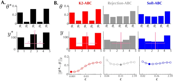
Toy problem We start by illustrating how the choice of summary statistics can significantly affect the inference result, especially when the summary statis-tics are not sufficient. We consider a symmetric Dirich-let prior πand a likelihood p(y|θ) given by a mixture of uniform distributions as π(θ) = Dirichlet(θ;1), p(y|θ) = 5 X i=1 θiUniform(y; [i−1, i]). (3)
The model parameters θ are a vector of mix-ing proportions. The goal is to estimate E[θ|y∗] where y∗ is generated with true parameter θ∗ = [0.25,0.04,0.33,0.04,0.34]> (see Fig. 1A). The sum-mary statistics are chosen to be empirical mean and variance i.e. s(y) = (ˆE[y],Vˆ[y])>.
We compare three ABC algorithms: K2-ABC3, rejec-tion ABC, and soft ABC. Here, soft ABC refers to an ABC algorithm which uses a similarity kernel in Eq. 1 withq= 2 andρ(y, y0) =ks(y)−s(y0)k2. For K2-ABC, we setM = 1000 and used a Gaussian kernel defined as k(a, b) = exp−ka−bk22 2γ2 to computeMMD\2 where γ is set to median({ky∗(i) −y∗(j) k}i,j) [29]. We test
different values of on a coarse grid, and report the estimated E[θ|y∗] which is closest to θ∗ as measured with a Euclidean distance.
The results are shown in Fig. 1 where the top row shows the estimated E[θ|y∗] from each method, asso-ciated with the bestas reported in the third row. The second row of Fig. 1, from left to right, showsy∗ and 400 realizations ofy drawn fromp(y|E[θ|y∗]) obtained from the three algorithms. In all cases, the mean and variance of the drawn realizations match that of y∗. However, since the first two moments are insufficient
3Code for K2-ABC is available at https://github.
com/wittawatj/k2abc.
to characterise p(y|θ∗), there exists other θ0 that can give rise to the same s(y0), which yields inaccurate posterior means shown in the top row. In contrast, K2-ABC taking into account infinite-dimensional suf-ficient statistic correctly estimates the posterior mean. Ecological dynamic systems As an example of statistical inference for ecological dynamic systems, we use observations on adult blowfly populations over time introduced in [20]. The population dynamics are modelled by a discretised differential equation:
Nt+1=P Nt−τexp −NNt−τ 0 et+Ntexp(−δt),
where an observation at timet+ 1 is denoted byNt+1 which is determined by time-lagged observations Nt
andNt−τ as well as Gamma distributed noise
realisa-tions et∼Gam(σ12 p, σ 2 p) and t∼Gam(σ12 d, σ 2 d). Here,
the parameters are θ = {P, N0, σd, σp, τ, δ}. We put
broad Gaussian priors on log of parameters as shown in Fig. 2A. Note that the time series data given the pa-rameters drawn from the priors vary drastically (see Fig. 2B), and therefore inference with those data is very challenging as noted in [30].
The observation (black trace in Fig. 2B) is a time-series of lengthT = 180, where each point in time in-dicates how many flies survive at each time under food limitation. For SL-ABC and K-ABC, we adopted the custom 10 summary statistics used in [30]: the log of the mean of all 25% quantiles of {Nt/1000}Tt=1 (four statistics), the mean of 25% quantiles of the first-order differences of {Nt/1000}Tt=1 (four statistics), and the maximal peaks of smoothed{Nt}Tt=1, with two differ-ent thresholds (two statistics). For IS-ABC, following [10], we use a Gaussian mixture model with three com-ponents as an auxiliary model. In addition, we ran two versions of SA-ABC algorithm on this example: SAQ regresses to simulated parameters from the corre-sponding simulated instances of time-series appended with the quadratic terms , i.e., g(y) = (y, y2)
∈R2T,
whereas SA-custom uses the above custom 10 sum-mary statistics from [30] appended with their squares as the candidate summary-statistics vectorg(y) (which is thus 20-dimensional in this instance).4
For setting and kernel parameters in K2-ABC, we split the data into two sets: training (75% of 180 data points) and test (the rest) sets. Using the training data, we ran each ABC algorithm given each value of
and kernel parameters defined on a coarse grid, then,
4For SL-ABC, we used the Python implementation by
the author of [30]. For IS-ABC, we used the MATLAB implementation by the author of [10]. For SA-ABC, we used the R packageabctoolswritten by the author of [8].
1 0 0.2 0.4 0 0 100 0 100 0 0.2 0.4 0.001 0.03 1 0 0.1 0.2 0.04 0.33 2.59 0.02 0.26 2.59 1 2 3 4 5 0 1 2 3 4 5 0 1 2 3 4 5 0 1 2 3 4 5
K2-ABC Rejection-ABC Soft-ABC
2 3 4 5
A.
B.
1 2 3 4 5 1 2 3 4 5 1 2 3 4 5
Figure 1: A possible scenario for ABC algorithms to fail due to insufficient summary statistics. A: Using the 5-dimensional true parameters (top), 400 observations (bottom) are sampled from the mixture of uniform distributions in Eq. 3. B (top): Estimated posterior mean of parameters from each method. We drew 1000 parameters from the Dirichlet prior and 400 simulated data points given each parameter. In rejection and soft ABC algorithms, we used empirical mean and variance of observations as summary statistics to determine similarity between simulated and observed data. B (middle): Histograms of 400 simulated data points given estimated posterior means by each method. Though the mean and variance of simulated data from rejection and soft ABC match that of the observed data, the shapes of the empirical distributions notably differ. B (bottom): Euclidean distance between true and estimated posterior mean of parameters as a function of . We varied the
values to find the optimal range in terms of the Euclidean distance. The magnitude ofis algorithm-specific and not comparable across methods.
computed test error5to choose the optimal values of and kernel parameters in terms of the minimum pre-diction error. Finally, with the chosen and kernel parameters, we ran each ABC algorithm using the en-tire data (M= 1000).
We show the concentrated posterior mass after per-forming K2-ABC in Fig. 2A, as well as an example trajectory drawn from the inferred posterior mean in Fig. 2B 6. To quantify the accuracy of each method, we compute the Euclidean distance between the vec-tor of chosen 10 summary statisticss∗=s(y∗) for the observed data ands(y) for the simulated dataygiven the estimated posterior mean ˆθ of the parameters. As shown in Fig. 3, K2-ABC outperforms other meth-ods, although SL-ABC, SA-custom, and K-ABC all
5We used Euclidean distance between the histogram
(with 10 bins) of test data and that of predictions made by each method. We chose the difference in histogram rather than in the realisation ofyitself, to avoid the error due to the time shift iny.
6Note that reproducing the trajectory exactlyis notthe
main goal of this experiment. We show the example tra-jectory to give the readers a sense of what the tratra-jectory looks like.
explicitly operate on this vector of summary statistics
swhile K2-ABC does not. In other words, while those methods attempt to explicitly pin down the parts of the parameter space which produce summary statistics
s similar tos∗, insufficiency of these summary statis-tics affects the posterior mean estimates undesirably even with respect to that very metric.
5
COMPUTATIONAL TRACTABILITYIn K2-ABC, given a dataset and pseudo dataset with n observations each, the cost for computing
\
MMD2(Fyi, Fy∗) is O(n
2). For M pseudo datasets, the total cost then becomes O(M n2), which can be prohibitive for a large number of observations. Since computational tractability is among the core consider-ations for ABC, in this section, we examine the per-formance of K2-ABC with different MMD approxima-tions which reduce the computational cost.
Linear-time MMD The unbiased linear-time MMD estimator presented in [17, section 6] reduces the total cost to O(M n) at the price of a higher
vari-0 5 K2-ABC SL-ABC −5 0 10 4 6 −4 0 4 −2 2 6 A. 0 180 0 1e4 K2-ABC SL-ABC K-ABC 1e4 1e4 time B. from prior 1e4 # flies 0 5 0 5 x103 x103 x103
Figure 2: Blowfly data. A (top): Histograms of 10,000 samples for four parameters{logP,logN0,logσp,logτ}
drawn from the prior. A (middle/bottom): Histogram of samples from the posteriors obtained by K2-ABC / SL-ABC (acceptance rate: 0.2, burn-in: 5000 iterations), respectively. In both cases, the posteriors over parameters are concentrated around their means (black bar). The posterior means of P and τ obtained from K2-ABC are close to those obtained from SL-ABC, while there is noticeable difference in the means of N0and
σp. Note that we were not able to show the same histogram for K-ABC since the posterior obtained by K-ABC
is improper. B (top): Three realisations of y given three different parameters drawn from the prior. Small changes inθdrastically changey. B (middle to bottom): Simulated data using inferred parameters (posterior means) shown in A. Our method (in red) produces the most similar dynamic trajectory to the actual observation (in black) among all the methods.
0 2 4 6 8
K2 SL SA-custom IS SAQ K-ABC
Figure 3: Euclidean distance between the chosen 10 summary statistics of y∗ and y given the posterior mean of parameters estimated by various methods. Due to the fluctuations in y from the noise realisa-tions (t, et), we made 100 independent draws ofyand
computed the Euclidean distance. Note that K2-ABC achieved nearly 50% lower errors than the next best method, SL-ABC, although SL-ABC, SA-custom, and K-ABC all explicitly operate on the summary statis-tics in the comparison while K2-ABC does not.
ance. Due to its computational advantage, the linear-time MMD has been successfully applied in large-scale two-sample testing [31] as a test statistic. The original linear-time MMD is given by \ MMD2l(Fx, Fy) = 2 n n/2 X i=1 k(x(2i−1), x(2i)) +k(y(2i−1), y(2i)) −k(x(2i−1), y(2i)) −k(x(2i), y(2i−1)) .
Note that we have assumed the same number of ob-servations nx = ny = n from Fx and Fy. The
esti-matorMMD\2l is constructed so that the independence
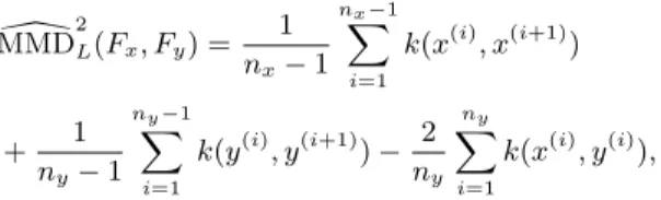
of the summands allows derivation of its asymptotic distribution and the corresponding quantile computa-tion needed for two-sample testing. However, since we do not require such independence, we employ a linear-time estimator with a larger number of sum-mands, which also does not require nx = ny.
With-out loss of generality, we assume nx ≤ ny Denote
x(j) := x(1+mod(j−1,nx)) for j > n
x, i.e., we allow a
cyclic shift through the smaller dataset{x(i) }nx
linear-time MMD estimator that we propose is \ MMD2L(Fx, Fy) = 1 nx−1 nXx−1 i=1 k(x(i), x(i+1)) + 1 ny−1 ny−1 X i=1 k(y(i), y(i+1))− 2 ny ny X i=1 k(x(i), y(i)),
which is an unbiased estimator of MMD2(Fx, Fy).
The total cost of the resulting K2-ABC algorithm is
O(M(nx+ny)).
MMD with random Fourier features Another fast linear MMD estimator can be achieved by consid-ering an approximation to the kernel functionk(x, y) with an inner product of finite dimensional feature vec-tors ˆφ(x)>φˆ(y) where ˆφ(x)∈RDandDis the number
of features. Given the feature map ˆφ(·) such that,
k(x, y)≈φˆ(x)>φˆ(y), MMD2can be approximated as MMD2rf(Fx, Fy)
≈EXφˆ(X)>EX0φˆ(X0) +EYφˆ(Y)>EY0φˆ(Y0)
−2EXφˆ(X)>EYφˆ(Y) :=kEXφˆ(X)−EYφˆ(Y)k22.
A straightforward (biased) estimator is
\ MMD2rf(Fx, Fy) = n1x nx X i=1 ˆ φ(x(i)) −n1 y ny X i=1 ˆ φ(y(i)) 2 2 ,
which can be computed in O(D(nx+ny)), i.e.,
lin-ear in the sample size, leading to the overall cost of
O(M D(nx+ny)).
Given a kernel k, there are a number of ways to ob-tain ˆφ(·) such thatk(x, y)≈φˆ(x)>φˆ(y). One approach which became popular in recent years is based on ran-dom Fourier features [32] which can be applied to any translation invariant kernel. Assume thatkis transla-tion invariant i.e.,k(x, y) = ˜k(x−y) for some function ˜
k. According to Bochner’s theorem [33], ˜kcan be writ-ten as ˜ k(x−y) = Z eiω>(x−y)dΛ(ω) =Eω∼Λcos(ω>(x−y)) = 2Eb∼U[0,2π]Eω∼Λcos(ω>x+b) cos(ω>y+b), where i = √−1 and due to positive-definiteness of ˜
k, its Fourier transform Λ is nonnegative and can be treated as a probability measure. By drawing ran-dom frequencies {ωi}Di=1 ∼Λ and {bi}Di=1 ∼U[0,2π], ˜
k(x−y) can be approximated with a Monte Carlo av-erage. It follows that ˆφj(x) =
p
2/Dcos(ω>
j x+bj)
and ˆφ(x) = ( ˆφ1(x), . . . ,φˆD(x))>. Note that a
Gaus-sian kernelkcorresponds to normal distribution Λ. Empirical results We employ the linear-time and the random Fourier feature MMD estimators in our
K2-ABC algorithm, which we callK2-linandK2-rf, re-spectively, and test these variants on the blowfly data. For K2-rf, we used 50 random features.
Figure 4: K2-ABC with different MMD estima-tors outperform the best existing method, SL-ABC, on the blowfly data. K2 K2-rf K2-lin SL 1 2 3 0
6
CONCLUSIONS
We investigated the feasibility of using MMD as a dis-crepancy measure of samples from two distributions in the context of ABC. Via embeddings of empirical data distributions into an RKHS, we effectively take into account infinitely many implicit features of these distributions as summary statistics. When tested on both simulated and real-world datasets, our approach obtained more accurate posteriors, compared to other methods that rely on hand-crafted summary statistics. While any choice of a characteristic kernel will guar-antee infinitely many features and no information loss due to the use of insufficient statistics, we note that the kernel choice is nonetheless important for MMD estimation and therefore also for the efficiency of the proposed K2-ABC algorithm. As widely studied in the RKHS literature, the choice should be made to best capture characteristics of given data, i.e., by utilising domain-specific knowledge. For instance, when some data components are believeda priorito be on differ-ent scales, one can adopt the automatic relevance de-temination (ARD) kernel instead of the Gaussian ker-nel. Formulating explicit efficiency criteria in the con-text of ABC and optimizing over kernel choice, simi-larly as in the context of two-sample testing [31], would be an essential extension.
Acknowledgments
We thank Arthur Gretton and Ted Meeds for their helpful comments. M Park and W Jitkrittum were funded by the Gatsby Charitable Foundation. M Park is grateful for the travel support by QUvA lab at Uni-versity of Amsterdam.
References
[1] S. Tavar´e, D. J. Balding, R. C. Griffiths, and P. Donnelly. Inferring coalescence times from DNA sequence data. Genetics, 145(2):505–518, 1997.
[2] O. Ratmann, O. Jørgensen, T. Hinkley, M. Stumpf, S. Richardson, and C. Wiuf. Using likelihood-free inference to compare evolu-tionary dynamics of the protein networks of H. pylori and P. falciparum. PLoS Computational Biology, 3(11):e230, 11 2007.
[3] E. Bazin, K. J. Dawson, and M. A. Beaumont. Likelihood-free inference of population structure and local adaptation in a bayesian hierarchical model. Genetics, 185(2):587–602, 06 2010. [4] C. M. Schafer and P. E. Freeman.
Likelihood-free inference in cosmology: Potential for the es-timation of luminosity functions. In Statistical Challenges in Modern Astronomy V, pages 3–19. Springer, 2012.
[5] P. Joyce and P. Marjoram. Approximately suffi-cient statistics and bayesian computation. Stat. Appl. Genet. Molec. Biol., 7(1):1544–6115, 2008. [6] C. P. Robert, J. Cornuet, J. Marin, and N. S.
Pil-lai. Lack of confidence in approximate Bayesian computation model choice. Proceedings of the National Academy of Sciences, 108(37):15112– 15117, 2011.
[7] M. Nunes and D. Balding. On optimal selection of summary statistics for approximate bayesian computation. Stat. Appl. Genet. Molec. Biol., 9(1):doi:10.2202/1544–6115.1576, 2010.
[8] P. Fearnhead and D. Prangle. Constructing sum-mary statistics for approximate Bayesian com-putation: semi-automatic approximate Bayesian computation.J. R. Stat. Soc. Series B, 74(3):419– 474, 2012.
[9] S. Aeschbacher, M. A. Beaumont, and A. Futschik. A Novel Approach for Choos-ing Summary Statistics in Approximate Bayesian Computation. Genetics, 192(3):1027–1047, 2012. [10] C.C. Drovandi, A.N. Pettitt, and A. Lee. Bayesian indirect inference using a parametric auxiliary model. Statist. Sci., 30(1):72–95, 02 2015.
[11] C.C. Drovandi, A.N. Pettitt, and M.J. Faddy. Ap-proximate Bayesian computation using indirect inference. J. R. Stat. Soc. Series C, 60(3):317– 337, 2011.
[12] A. Gleim and C. Pigorsch. Approximate Bayesian computation with indirect summary statistics.
Draft paper: http://ect-pigorsch. mee. uni-bonn. de/data/research/papers, 2013.
[13] Gael M. Martin, Brendan P. M. McCabe, Worapree Maneesoonthorn, and Christian P. Robert. Approximate Bayesian Computation in State Space Models. arXiv:1409.8363 [math, stat], September 2014. arXiv: 1409.8363.
[14] A. Berlinet and C. Thomas-Agnan. Reproducing Kernel Hilbert Spaces in Probability and Statis-tics. Kluwer, 2004.
[15] A. Smola, A. Gretton, L. Song, and B. Sch¨olkopf. A Hilbert space embedding for distributions. In
ALT, pages 13–31, 2007.
[16] B. Sriperumbudur, K. Fukumizu, and G. Lanck-riet. Universality, characteristic kernels and RKHS embedding of measures. J. Mach. Learn. Res., 12:2389–2410, 2011.
[17] A. Gretton, K. Borgwardt, M. Rasch, B. Sch¨olkopf, and A. Smola. A kernel two-sample test. J. Mach. Learn. Res., 13:723–773, 2012.
[18] L. Song, K. Fukumizu, and A. Gretton. Kernel embeddings of conditional distributions. IEEE Signal Process. Mag., 30(4):98–111, 2013. [19] D. Sejdinovic, H. Strathmann, M.G. Lomeli,
C. Andrieu, and A. Gretton. Kernel Adaptive Metropolis-Hastings. InICML, 2014.
[20] S. N. Wood. Statistical inference for noisy nonlinear ecological dynamic systems. Nature, 466(7310):1102–1104, 08 2010.
[21] S. Nakagome, K. Fukumizu, and S. Mano. Ker-nel approximate bayesian computation in popula-tion genetic inferences. Stat. Appl. Genet. Molec. Biol., 12(6):667–678, 2013.
[22] S. Gr¨unew¨alder, G. Lever, A. Gretton, L. Baldas-sarre, S. Patterson, and M. Pontil. Conditional mean embeddings as regressors. InICML, 2012. [23] D. Sejdinovic, B. Sriperumbudur, A. Gretton, and
K. Fukumizu. Equivalence of distance-based and RKHS-based statistics in hypothesis testing.Ann. Statist., 41(5):2263–2291, 2013.
[24] A. Christmann and I. Steinwart. Universal kernels on non-standard input spaces. In NIPS, pages 406–414, 2010.
[25] Z. Szab´o, A. Gretton, B. P´oczos, and B. Sripe-rumbudur. Two-stage Sampled Learning The-ory on Distributions. ArXiv e-prints:1402.1754, February 2014.
[26] M.C. Wu, P. Kraft, M.P. Epstein, D.M. Taylor, S.J. Chanock, D.J. Hunter, and X. Lin. Powerful SNP-Set Analysis for Case-Control Genome-wide
Association Studies. The American Journal of Human Genetics, 86(6):929–942, June 2010. [27] S. Li and Y. Cui. Gene-centric genegene
inter-action: A model-based kernel machine method.
Ann. Appl. Stat., 6(3):1134–1161, September 2012.
[28] T. G¨artner. A survey of kernels for structured data. SIGKDD Explor. Newsl., 5(1):49–58, July 2003.
[29] B. Sch¨olkopf and A. J. Smola.Learning with Ker-nels: Support Vector Machines, Regularization, Optimization, and Beyond. MIT Press, Cam-bridge, MA, USA, 2001.
[30] E. Meeds and M. Welling. GPS-ABC: Gaussian Process Surrogate Approximate Bayesian Com-putation. In UAI, volume 30, pages 593–601, 2014.
[31] A. Gretton, , B.K. Sriperumbudur, D. Sejdinovic, H. Strathmann, S. Balakrishnan, M. Pontil, and K. Fukumizu. Optimal kernel choice for large-scale two-sample tests. InNIPS, pages 1205–1213. 2012.
[32] A. Rahimi and B. Recht. Random features for large-scale kernel machines. InNIPS, pages 1177– 1184, 2007.
[33] Walter Rudin. Fourier Analysis on Groups: In-terscience Tracts in Pure and Applied Mathemat-ics, No. 12. Literary Licensing, LLC, 2013.