Efficient search in graph databases using cross filtering
Chun-Hee Lee, Chin-Wan Chung
⇑Department of Computer Science, KAIST, Daejeon 305-701, Republic of Korea
a r t i c l e
i n f o
Article history: Received 6 June 2013
Received in revised form 13 May 2014 Accepted 26 June 2014
Available online 16 July 2014 Keywords: Graph indexing Simple feature Graph feature Cross filtering
a b s t r a c t
Recently, graph data has been increasingly used in many areas such as bio-informatics and social networks, and a large amount of graph data is generated in those areas. As such, we need to manage such data efficiently. A basic, common problem in graph-related applica-tions is to find graph data that contains a query (Graph Query Problem). However, since examining graph data sequentially incurs a prohibitive cost due to subgraph isomorphism testing, a novel indexing scheme is needed.
A feature-based approach is generally used as a graph indexing scheme. A path structure, a tree structure, or a graph structure can be extracted from a graph database as a feature. The path feature and the tree feature can be easily managed, but have lower pruning power than the graph feature. Although the graph feature has the best pruning power, it takes too much time to match the graph feature with the query. In this paper, we propose a graph feature-based approach called a CF-Framework (Cross Filtering-Framework) to solve the graph query problem efficiently. To select the graph features that correspond to the query with a low cost, the CF-Framework makes two feature groups according to the query and filters out each group crossly (i.e., alternately) based on set properties. We then validate the efficiency of the CF-Framework through experimental results.
Ó2014 Elsevier Inc. All rights reserved.
1. Introduction
Graph data has been used for a long time in computer science in order to represent various structures; many techniques related to graphs have been developed and utilized. Recently, due to technological advances, a large amount of graph data has been generated in broader areas. For example, in a social network environment, a very large social network is produced. In addition, in the bio-informatics area[12], various protein structures are modeled by a labeled graph. However, since the previous research related to graphs focuses on a small amount of data, this cannot be applied to a large amount of graph data. In the case of XML data similar to graph data, research on large-scale XML data management has been studied very actively [4,9,24,19,6,16,18]. However, XML data is primarily represented by a tree structure and XML’s abundant technologies cannot be applied to graph data directly. Therefore, database communities are trying to overcome the scalability issue of graph data. Data retrieval is a basic and common technique among the graph data management techniques. An important graph data retrieval problem is to find graph data that contains a graph query. We call this the graph query problem. The graph query problem is formally defined as follows:
http://dx.doi.org/10.1016/j.ins.2014.06.047 0020-0255/Ó2014 Elsevier Inc. All rights reserved.
⇑Corresponding author.
E-mail addresses:[email protected](C.-H. Lee),[email protected](C.-W. Chung).
Contents lists available atScienceDirect
Information Sciences
Given a graph databaseD¼ fg1;g2;. . .;gngand a graph queryq, find all graphsdinDsuch thatqd.1
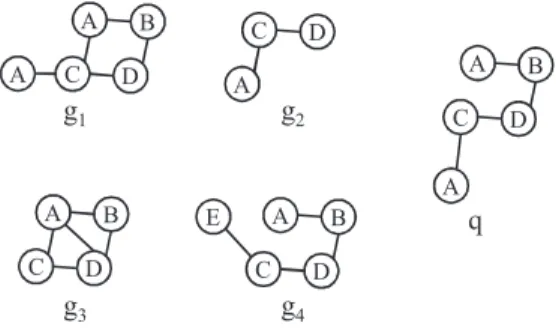
Example 1.SupposeD¼ fg1;g2;g3;g4gand that the graph query isqas shown inFig. 1. The answer of the queryqisg1since g1is a supergraph ofq. In this example, we omit edge labels.
It is not possible to scan the whole data inDsince subgraph isomorphism testing is an NP-complete problem[5]. To solve the graph query problem, a feature-based approach is generally used. In the feature-based approach, to find the graph datad that contains the queryq(i.e.,dq), we make the feature index and compute the candidate result using the index.hf;Dfiis used as an index structure, wherefis some feature extracted fromDandDf ¼ fd2Djfdg. Then, given a queryq, the can-didate answer set (Cq) is computed using the precomputed list ofhfi;Dfii. Iffiq, thenDfiDq. Thus, the intersection of the Dfi’s is a superset ofDq, wherefiis a feature andfiq. Therefore, we can computeCqby the formulaCq¼ \fiq and fi2FDfi, whereF is a set of features. Finally, we get real answers by directly checking whether d2Cq is a real answer. In the feature-based approach, the query processing cost is mainly affected by two kinds of costs; the index probing cost and the verification cost. The index probing cost is the cost of finding the list of features that match the query and the verification cost is the cost of checking whether a candidate answer is a real answer.
In the GraphGrep[21,8], a path is used as a feature. Although we can extract paths easily and compare two path sets extracted from the query and the graph data with a low cost, the pruning power for paths is low. This means that the index probing cost for the path feature is low, but the verification cost is very high due to the big size of the candidate answer set. To reduce the verification cost, we can use a graph feature instead of a path feature. In the gIndex[29], a frequent and discriminative subgraph is selected as a feature. However, the index probing cost is high in the gIndex since the gIndex has to find the graph features that are contained in the query and it requires subgraph isomorphism testing.
In the FG-index[2], to remove the verification cost, the exact answer set corresponding to queryqis retrieved in the index probing step. If the same featurefas the queryqis found, the precomputedDfis returned as a result. Then, query processing can be performed without the verification step of checking the candidate answer since the exact answers are matched. How-ever, in order to compute an answer of the query without verification, the query should be in the feature set. In case the query is not in the feature set, it is not efficient to process the query. To avoid such a case, the FG-index should make the feature index for a very large number of subgraphs, which will increase the index probing cost.
In summary, in the case of using a path feature, we have the problem of low pruning power. Therefore, we have a high verification cost. In case of using a graph feature, we should find the graph features that match with the graph query. There-fore, we have a high index probing cost. To solve this dilemma, we propose the CF-Framework (Cross Filtering-Framework). Since graph features are used in the CF-Framework, we can get a low verification cost. In addition, to efficiently find the graph features contained in the query, we propose a filtering method called Cross Filtering. Using Cross Filtering, we can achieve a low index probing cost. In Cross Filtering, to find the graph features contained in the query, we make two different feature groups for the query. Then, using set properties, each group is filtered out crossly (i.e., alternately). We then perform the filtering iteratively until we search all features. During this process, we can select the graph features that correspond to the query efficiently and therefore reduce the index probing cost.
In addition, to process the graph query more effectively, the CF-Framework provides a two-step architecture to compute candidate answers. In the first candidate answer computation, we evaluate a loose candidate answer set with a small cost using features that are easy to compute; we call them simple features. In the second candidate answer computation, we compute a tight candidate answer set using graph features and the result of the first candidate answer computation. In this step, we perform Cross Filtering.
A C D A B
g
1 A C Dg
2 C D A Bg
3 E C D A Bg
4 A C D A Bq
Fig. 1.Example for the graph query problem.
1
Formally, for graph datag1andg2;g1g2means thatg1andg2have a subgraph isomorphism fromg1tog2. For convenience, we say thatg1is a subgraph
ofg2ifg1g2. We will define the subgraph isomorphism formally in Section3. Also, note that we use the symbolinstead of the symbol#to indicate
1.1. Contributions
Our contributions are as follows:
Efficient graph feature filtering method (Cross Filtering).Although a graph feature has a high pruning power, it is hard to find the graph features contained in a query. To overcome the problem, we propose Cross Filtering. By filtering out graph features crossly and iteratively based on the derived set properties, Cross Filtering can select graph features efficiently.
CF-Framework to process a graph query.We propose an effective framework to process a graph query using simple fea-tures and graph feafea-tures. We first compute a loose candidate answer set very efficiently using simple feafea-tures, and then we compute a tight candidate answer set using graph features and the above candidate answer set.
Experimentation to validate our proposed approach.Through an experimental study using a real dataset, we show that the CF-Framework can process graph queries efficiently. For various types of queries, the CF-Framework outperforms the previous approach in most cases in terms of the query processing time.
1.2. Organization
The rest of the paper is organized as follows. We discuss related work in Section2and explain the preliminary concepts and the overall procedure in Sections3 and 4, respectively. We describe the first candidate answer computation using simple features in Section5, then we present the second candidate answer computation using graph features in Section6. Finally, we show experimental results in Section7and conclude the paper in Section8.
2. Related work
XML data is similar to graph data. We can generally express XML data as a tree, a subset of a graph, and if we use IDREF, the XML data will become a graph. To process XML data, various indexing and query processing techniques have been pro-posed[4,9,24,19,6,16,18,13,28]. However, they focus on XML data that has a tree structure. Thus, the techniques studied in the XML area cannot be easily adapted to graph data. Therefore, many approaches are proposed in order to deal with graph data[21,8,29,2,3,38,14,11,27,37,7,15].
To process graph data efficiently, Shasha et al.[21,8]proposed a path-based approach. All paths within the maximum path length are extracted from a database and indexed. Given a query, the paths corresponding to it are retrieved and a can-didate answer set is computed using the paths. However, in the path-based approach, the filtering capability of the paths will be degraded compared to that of the graph since the path loses the structural information of the graph.
As an alternative to paths, frequent subgraphs can be used as a good feature set. Subgraphs can preserve the structural information of the original graph data. However, the number of subgraphs can be very large. In the gIndex[29], to reduce the size of the feature set, frequent and discriminative subgraphs are selected among many subgraphs. The key idea in the gIn-dex is that if two featuresf1andf2have a subgraph relationship (f1f2) and similar frequencies, we do not have to keep both
f1andf2. Using this idea, the gIndex can reduce the size of the feature set. However, the gIndex has difficulty finding the
feature list contained in queryq.
We have the high verification cost to process the graph query due to the subgraph isomorphism testing. The FG-index[2] can avoid the verification cost if the index contains the graph query. For a non-FG-query that is not contained in the index, the query performance of the FG-index is not efficient. To process many types of queries without verification, the FG-index should construct the index with a very large number of subgraphs. However, since the number of possible subgraphs is incredibly large, there may still be many non-FG queries. The FG⁄
-index[3]proposes an FAQ-index to solve the problem. If the non-FG-query is in the FAQ-index which is dynamically built from the set of frequently asked non-FG-queries, then the FG⁄-index returns the result of the non-FG-query without verification. However, the essential problem of the FG-index
cannot be avoided.
In GCoding[38], a novel encoding method for graph indexing is proposed. In GCoding, graph data is encoded into graph code by combining all the vertex signatures that represent the local structure around a vertex. For effective encoding of the local structure around a vertex, the interlacing theorem for eigenvalues is utilized. However, GCoding has the limitation of representing an intrinsic property of a graph, since structural information may be lost during the encoding. Therefore, its filtering capability may be degraded compared to approaches that use frequent subgraphs.
In addition, many kinds of graph search techniques that are in contexts different from ours have been studied. Similar graph search techniques are proposed in[10,26,30,25,17,23]. The containment search technique[1]is devised using a con-trast subgraph. Yuan et al. dealt with the subgraph search problem and a similar subgraph search problem in an uncertain graph database[33,34]. In[36,35,22], the subgraph search in a single large graph instead of a collection of graph data is pro-posed. GraphREL[20]provides a framework to store and query graph data in an RDBMS. In addition, a method to update a graph index incrementally is proposed in[32,31]while many approaches do not consider the environment in which a graph index is updated. In particular, Yang and Jin[31]consider the graph search problem for a single large graph in a dynamic
environment where nodes or edges are inserted or deleted over time. They partition the graph into core regions and extend these core regions to index regions in order to reduce the update time of the indices.
3. Preliminary
In this section, we describe notations and the basic lemma. A graph consists of vertices and edges. We can represent the graph byG¼ hV;E;L;li, whereVis the set of vertices,Eis the set of edges,Lis the set of vertex and edge labels andlis a function from a vertex or an edge to a label inL. In this paper, we consider an undirected, labeled graph. In addition, we assume that both the nodes and edges have labels.
Definition 1. For any two graphsg1¼ hV;E;L;liandg2¼ hV0;E0;L0;l0i, we say thatg1g2if there exists an injective function f:V!V0 such that (1) for all
v
2V;fð
v
Þ 2V0 and lð
v
Þ ¼l0ðfðv
ÞÞ, and (2) for all hv1
;v2
i 2E;hfðv1
Þ;fðv2
Þi 2E0 andlðh
v1
;v2
iÞ ¼l0ðhfðv1
Þ;fðv2
ÞiÞ. We callfthe subgraph isomorphism fromg1tog2.As mentioned previously, since the subgraph isomorphism testing is an NP-complete problem[5], we construct the index to reduce the computation of query processing. Given queryq, featuref, and graph databaseD, we defineDf anddf as follows:
Df¼ fg2Djgfg df ¼ fg2Djgfg
We can evaluate a candidate answer set basically by usingDf. In addition, to compute a tighter candidate answer set, we can usedf as well which will be explained in Section6.3.
The following lemma can be derived easily from the definition ofDf. Lemma 1. For any two graphs g1and g2, if g1g2, Dg1Dg2.
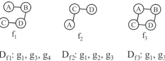
ByLemma 1, we can compute a candidate answer setCqby intersectingDf’s forfq, whereqis a query. For example, suppose thatf1;f2, andf3inFig. 2are the graph features extracted fromg1,g2;g3, andg4inFig. 1and the queryqinFig. 1is
given. Then,f1andf2are contained inq. Therefore,Cq¼Df1 T
Df2¼ fg1;g3g.
4. Overall procedure
In this section, we describe the overall procedure. In a graph feature-based approach, there are two major steps in pro-cessing the graph query problem, the first of which is the index construction step. In this step, it is important to extract use-ful graph features from a graph database. Many papers deal with a method of extracting effective graph features[29,37]; therefore, in this paper we do not focus on extracting graph features. Instead, we assume that the graph features are given. The second step is a query processing step. Query processing consists of the first candidate answer computation, the sec-ond candidate answer computation and the verification. In the first candidate answer computation, we evaluate a loose can-didate answer set in a very short time using simple features. In the second cancan-didate answer computation, we evaluate a tight candidate answer set using graph features and the above result.
However, since we need much time to find the graph features contained in the query in the second candidate answer computation, we propose Cross Filtering. To find the graph features efficiently in Cross Filtering, we compute Group1 and Group2 using simple features2and the computation cost is low. Group1 and Group2 are defined as follows:
Group1Fsub¼ ffjf2F;f qg; whereF¼graph feature set; q¼query Group2Fsup¼ ffjf2F;f qg; whereF¼graph feature set; q¼query
By crossly filtering out the graph features from Group1 and Group2, we can get the graph features contained in the query efficiently. In the verification, which is the final process of query processing, we verify the candidate answers to get the real answers. The detailed algorithm is shown inFig. 5, which will be explained in Sections5 and 6.
C D A B
f
1 A C Df
2D
f1: g
1, g
3, g
4D
f: g
1, g
2, g
3 C D A Bf
3D
f3: g
1, g
3 2Fig. 2.Graph feature example forg1;g2;g3andg4inFig. 1.
2
Although we have proposed simple features in this paper, these are only some of simple feature examples. In fact, we can use various graph-theoretical properties as simple features that have been proposed in graph theory communities. However, our focus is not on finding a good simple feature. In this paper, we will concentrate on the second candidate answer computation.
5. First candidate answer computation using simple features
In this section, we will explain the first candidate answer computation (Lines 2–8 ofFig. 5). 5.1. Simple features
To evaluate a candidate answer set with a small cost, we use simple features that are easy to compute. A simple feature has the following characteristics:
Small extraction time.The feature extraction time from a graph should be small. If the time is long, the index construc-tion and query processing will be performed badly.
Small space.We should store the value of the simple feature with a small amount of space. If the space size of storing the simple feature is large, the index size will be large.
Subgraph property.The simple feature should satisfy the subgraph property below; if the simple feature does not have this property, we cannot compute candidates through simple features. This property is the most important property for simple features.
Definition 2 (Subgraph Property). Let sfi be a function from the graph data to some values (i.e., real numbers). If sfiðg1Þ sfiðg2Þfor any two graph datag1andg2such thatg1g2, we say thatsfihas the subgraph property. The operator is a user-defined operator for comparing the two values. In general, the relation6is used.
Many simple features satisfy the above three properties. As a typical example, we use the number of vertices (nV) and the number of edges (nE). For any two graphsg1andg2, ifg1g2;nVðg1Þ6nVðg2ÞandnEðg1Þ6nEðg2Þ. Furthermore,nVandnE
have a small extraction time and the values of those take a small space; therefore,nVandnEare simple features. According to the properties of the graph data, various kinds of good simple features exist. A good simple feature means a feature with high discriminative power. However, it is difficult to find good simple features for all kinds of graph data sets. Therefore, we can determine the simple features with the help of a domain expert.
In this paper, we do not focus on finding good simple features. Instead, we describe simple feature examples that can be used in a general environment inAppendix A.
5.2. Candidate answer computation using simple features
As explained in the overall procedure, we first compute a loose candidate answer set using simple features. We will explain Lines 2–8 ofFig. 5in detail.
Given a queryq, we first extract the values of the simple features ofq;sfðqÞ(Line 2 ofFig. 5). The functionsfðxÞis defined by½sf1ðxÞ;sf2ðxÞ;. . .;sfkðxÞ, wherekis the number of simple features. Then, we evaluate the candidate answer set using the
formulaCq¼ fg2DjsfðqÞ sfðgÞg(Line 3 ofFig. 5). SincesfðqÞis a vector, we definein a vector. IfsfðgÞ ¼ ð
v
1;v
2;. . .;vk
Þandsfðg0Þ ¼
v
01;
v
02;. . .;v
0k
, thensfðgÞ sfðg0Þmeans
v
1
v
01ANDv
2v
20 AND ANDvk
v
0k, whereis defined in each simple feature.3We are sure thatCqis a superset ofDqbecause simple features have the subgraph property that states that for any two graphsg1andg2, ifg1g2, thensfðg1Þ sfðg2Þ. If the size ofCqis small, we do not proceed with the second answer setcomputation (Lines 4–8 ofFig. 5). If we design simple features well, we can process graph queries easily with only simple fea-tures. However, in general cases, since the discriminative power of simple features is low, we need to use graph feafea-tures. 6. Second candidate answer computation using graph features
In this section, we will explain the second candidate answer computation (Lines 10–18 ofFig. 5) including the verification (Lines 19–21 ofFig. 5).
6.1. Graph features
Although simple features are easy to manage, the discriminative power of simple features may be low. Then we cannot effectively filter out graph data. It may be impossible to find simple features with high discriminative power for all kinds of
3
In our experimental setting, we use 5 simple features (i.e., the number of nodes, the number of edges, maximum degree, vertex encoding of Appendix, and edge encoding of Appendix).
graph data sets. Therefore, we use frequent subgraphs as a good feature additionally. However, we have difficulty managing graph data. Thus, an efficient graph feature filtering method should be devised.
6.2. Candidate answer computation using graph features
To compute a tight candidate answer setCq, we use graph features that are a set of special subgraphs. However, we have difficulty dealing with graph features while simple features are easy to handle. We propose a method called Cross Filtering to find the graph features contained in the query efficiently and integrate it with query processing. In the Cross Filtering, we compute the candidate answer set as well as the partial answer set. The partial answer set Pq is defined by
Pq¼ [fiq and fi2FDfi, whereFis the feature set.Fig. 3(a) shows the relationship amongCq,PqandDq. We do not have to verify
Pqbecause all elements inPqare in the real answer set. Therefore, we only have to check whether the elements inCqPqare in the real answer set. As the final result, we return (the result of verification)[Pq. The FG⁄-index[3]also uses a partial
answer set. If the query is not in the FG⁄-index, the FG⁄-index uses the FAQ-index which is dynamically built from the set
of FAQs (Frequently Asked non-FG-Queries). If the query does not match with the FAQ-index, the FG⁄-index findsq’s
sub-graphs and supersub-graphs, then computes a candidate answer set and a partial answer set. However, it is inefficient to find graph featuresfsðqÞandftðqÞfor computing the candidate answer and the partial answer in the FG⁄-index. In Cross
Fil-tering, we devised a smart method to findfsandftsimultaneously.
Consider a graph featurefandDf ¼ fd2Djfdg ¼ fgi1;gi2;. . .;ging. AlthoughDf consists of graph data, we store a set of graph identifiers instead of a set of graph data. That is, we storeDf ¼ fi1;i2;. . .;ing, whereikis the identifier for graphgik (16k6n). Therefore, it is easier to deal withDf thanfsinceDf is a set of numbers andfis a graph. Furthermore,Dfexploits the characteristics offwell. Thus, to avoid the high computation for graph comparison, we useDf instead offand derive some formulas related toDf.
In Cross Filtering, we first compute the initial Group1 and Group2 using simple features. Since we use simple features, the computation cost to get the initial Group1 and Group2 is ignorable. This example will be shown in detail in Step 1 of Example 2.
Real Answer Set Dq
Candidate Answer Set Cq
Partial Answer Set Pq
P
qD
qC
q(a) Relationship
(b) Iteration
Fig. 3.Cq;DqandPq.Initial Group1¼ ffjf2F;sfðfÞ sfðqÞg. Group1 contains subgraphs ofqinF. That is, all elementsf2Fsuch thatfqare contained in Group1.4
Initial Group2¼ ffjf2F;sfðqÞ sfðfÞg. Group2 contains supergraphs ofqinF. Therefore, all elementsf2Fsuch that fqare contained in Group2.
In each group, to find a set offsðqÞand a set offtðqÞefficiently, we deriveLemma 3andLemma 4. Lemma 2. For any two graphs g1and g2, if Dg1 6 Dg2then g1 åg2.
Proof. Lemma 2is the contraposition ofLemma 1. h
Based onLemma 2, we are sure that ifDf1 6 Df2;f1is not a subset off2. For example, suppose thatDf1¼ f1;2;3;4;5gand Df2¼ f1;2;3;6g. SinceDf1 6 Df2, it is true thatf1 åf2.
Considerfssuch thatfsq. Forf2F(F: graph feature set), ifDfs 6 Df, we can say thatfs åf. Then, what relationship doq andfhave?
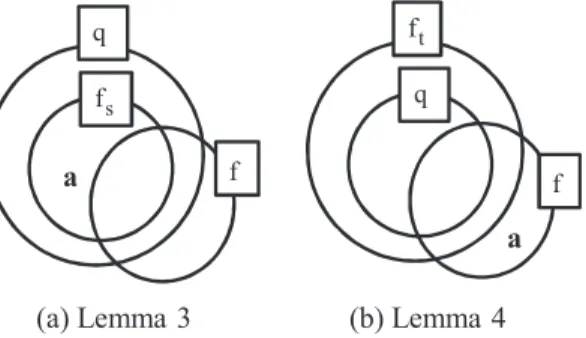
Lemma 3. If fsq and Dfs 6 Df, then qåf .
Proof. ByLemma 2,fs åf. Sincefs å f, there existsa2fssuch thata R fas shown inFig. 4(a). Sincefsq;a2q. Bya2q anda R f;qå f.5 h
In the same way, we can considerftsuch thatftq. Forf2F, ifDft å Df;ft 6 f. What relationship doqandfhave in this case?
Lemma 4. If ftq and Dft åDf, then q6 f .
Proof. ByLemma 2,ft 6 f. Sinceft 6 f, there existsa2fsuch thata R ftas shown inFig. 4(b). Sinceftq;a R q. Bya2f anda R q;q6f. h
ByLemma 3, ifDfs 6 Df, wherefsq, thenqå f. Furthermore, byLemma 4, ifDft åDf, whereftq, thenq6 f. By using the concepts, we devise an efficient graph feature filtering algorithm which can be integrated with the query process-ing algorithm.
In order to perform filtering for graph features, we choose one featurefsðqÞfrom Group1. We compute candidates using Cq¼Cq\Dfs, then we reevaluate Group1 and Group2 as follows: GivenfsðqÞ,
Group1:¼ ff2Group1jDf 6Dfsg.
Group2:¼ ff2Group2jDf Dfsg.
We filter out a featuref2Group1 such thatDf Dfs, becauseDf cannot reduce the size ofCqin that case (See Group1 in Step 2 ofExample 2). In addition, since ifDfs 6Dfthenqåf(byLemma 3), we can filter out a featurefin Group2 such that Df å Dfs (See Group2 in Step 2 ofExample 2).
f
sf
q
a
q
f
f
ta
(a) Lemma 3
(b) Lemma 4
Fig. 4.Relationship between the graphs.
4
For convenience, featurefwith the same simple feature values as the query is contained in Group1.
5
Strictly speaking, we cannot use the notationa2gfor graphgsince graphgis not a set. However, since a graph consists of a set of vertices and a set of edges, it can be used in our mathematical proof.
Next, we choose one featureftðqÞfrom Group2.Dft is a partial answer ofDqsince ifftqthenDftDq(byLemma 1). We compute the partial answer setPqwithftby computingPq¼Pq[Dft. Then, usingft, we reevaluate two groups as follows:
Group1:¼ ff2Group1jDfDftg.
Group2:¼ ff2Group2jDf åDftg.
We removef2Group1 such thatDf 6 Dftsince ifDft åDfthenq6 fbyLemma 4(See Group1 in Step 3 ofExample 2). In a similar way to that offs, we compute Group2. IfDf Dft;Dfcannot increase the size ofPq. Therefore, we add the condition Df åDft when evaluating Group2 (See Group2 in Step 3 ofExample 2).
We perform the above two procedures iteratively until we have searched all features. The subset selection (fs) and the superset selection (ft) are performed in turn while effectively reducing the size of each group. Through the subset selection (fs),Cqis reduced iteratively and through the superset selection (ft),Pqis increased iteratively as shown inFig. 3(b).
The second candidate answer computation with Cross Filtering is summarized in Lines 10–18 ofFig. 5. In Line 10, the partial answer set is initialized. Two groups, Group1 and Group2, are made using the simple features in Line 11, we then perform the two steps iteratively until we have searched all the features in Lines 12–18. In Lines 13–15, filtering andCq com-putation are performed withfs. In Lines 16–18, filtering andPqcomputation are performed withft. Finally, we do the veri-fication on onlyCqPqand return the result (Lines 20–21).
In the algorithm ofFig. 5, we choose a seed subgraph feature (fs) or a seed supergraph feature (ft) of the graph query using a sequential selection and subgraph isomorphism checking (Lines 13 and 16). We choose one element in Group1 (or Group2) and check the subgraph isomorphism between the element and the graph query. If they do not have a subgraph relationship, we choose another element. At this time, we may not abandon the information that they do not have a subgraph relation-ship. Using additional filtering that will be explained in Section6.3, we can further reduce Group1 and Group2. In addition,
during the iteration of Cross Filtering, the sizes of Group1 and Group2 are continuously being reduced by filtering out unnec-essary graph features.
However, we can use a heuristic selection method to reduce the time spent selecting a seed subgraph feature (fs) or a seed supergraph feature (ft) of the graph query. For example, we can sort graph features by the number of nodes and choose a graph feature in ascending or descending order. An elegant heuristic selection method will be our future work.
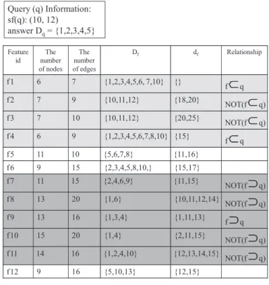
Example 2. Fig. 6shows 12 graph features and their properties. In this example, we use the number of vertices and the number of edges as simple features. Df is the precomputed index andRelationship shows the relationship between the feature and the query.df is used inExample 3. We assume that the initialCq¼ fg1;g2;g3;g4;g5;g6;g7;g8;g9;g10g.
Step 1 : We make two groups, Group1 and Group2, using two simple features. Since the simple features of the query are (10,12), Group1¼ ff1;f2;f3;f4gand Group2¼ ff7;f8;f9;f10;f11g.f5;f6andf12are filtered out.
Step 2: We selectf1ðqÞfrom Group1 asfs. Then,Cq¼Cq\Df1¼ fg1;g2;g3;g4;g5;g6;g7;g10g, then we filter out Group1 and
Group2 usingf1. SinceDf4 in Group1 is a superset ofDf1;f4is filtered out andf7is filtered out due to the fact that Df7 å Df1. Therefore, Group1¼ ff2;f3gand Group2¼ ff8;f9;f10;f11g.
Step 3: We checkf8from Group2 in order to chooseft. However, we removef8from Group2 sincef86 q. Next, we select
f9ðqÞfrom Group2. We computePq¼Pq[Df9¼ fg1;g3;g4g. Usingf9, we reevaluate Group1 and Group2.Df2 and Df3do not includeDf9; therefore, they are removed from Group1. In addition,Df10Df9; therefore,Df10is removed from Group2. Then, Group1¼ fgand Group2¼ ff11g.
Step 4: We checkf11and remove it. Then, Group1¼ fgand Group2¼ fg.
Step 5: Since Group1¼ fgand Group2¼ fg, we stop filtering.Cq¼ fg1;g2;g3;g4;g5;g6;g7;g10gandPq¼ fg1;g3;g4g.
There-fore, we verifyCqPq¼ fg2;g5;g6;g7;g10g. We get thefg2;g5gfrom the verification and returnfg2;g5g [ fg1;g3;g4g.
6.3. Additional filtering
In this subsection, we will provide tighter formulas for evaluating Group1 and Group2 than those in Line 18 ofFig. 5. Therefore, we can filter out Group1 and Group2 more effectively. In Line 16, to choose one featureft, we should check ele-ments in Group2 sequentially until we findftq. Then, we can get a list of featureshfiisuch thatfi 6 qduring the execution of Line 16. To provide tighter formulas, we use this information. Assume thatNAqis a non-answer set such thatd6 qfor all d2NAq. Then, we can derive the following two lemmas with respect toNAq.
Feature id The number of nodes The number of edges Df df Relationship f 1 6 7 {1,2,3,4,5,6, 7,10} {} f q f 2 7 9 {10,11,12} {18,20} NOT(f q) f 3 7 10 {10,11,12} {20,25} NOT(f q) f 4 6 9 {1,2,3,4,5,6,7,8,10} {15} f q f 5 11 10 {5,6,7,8} {11,16} f 6 9 15 {2,3,4,5,8,10,} {15,17} f 7 11 15 {2,4,6,9} {11,15} NOT(f q) f 8 13 20 {1,6} {10,11,12,14} NOT(f q) f 9 13 16 {1,3,4} {1,11,13} f q f 10 15 20 {1,4} {2,11,15} NOT(f q) f 11 14 16 {1,2,4,10} {12,13,14,15} NOT(f q) f 12 9 16 {5,10,13} {12,15}
Query (q) Information:
sf(q): (10, 12)
answer D
q= {1,2,3,4,5}
Lemma 5. If Df\NAq–/;qåf .
Proof. Consider the contraposition of this lemma. That is, ifqf, thenDf\NAq¼/. Ifqf;DqDf. SinceDf is a subset of the answer setDq, all elements inDf are not inNAq. h
Lemma 6. If Df NAq andjDqj–0, then f åq.
Proof. Consider the contraposition of this lemma. That is, we prove iffq, thenDf å NAqorjDqj ¼0. There are two cases. Case 1: jDqj ¼0. In this case, it is trivial.
Case 2: jDqj–0. IfjDqj–0, thenDqhas at least one element (i.e., one answer).
Iffq, thenDfDq. Therefore,Df contains all answers forq. Therefore,Df has at least one answer. This means that
Df åNAq. h
Using the above two lemmas, we can revise the computation of Group1 and Group2 in Line 18 ofFig. 5as follows: Group1:¼ ff2Group1jDfDft andðDf åNAqorjDqj ¼0Þg.
Group2:¼ ff2Group2jDf åDft and DfTNAq¼/g.
If a partial answer set is not null, thenjDjis not zero. Therefore, instead of the conditionjDqj ¼0, we can use the condition jPqj ¼0 since checking the conditionjDqj ¼0 is not straightforward. We can filter out graph features further. However, com-puting a non-answer set is not straightforward since we keep only Df. To get NAq, we compute df ¼ fg2Djgfg additionally.
Lemma 7. If qåf , then, for all x2df;x: q. That is, dfNAq.
Proof. Whenf 6 q, there existsa2qsuch thata R f. Therefore, a subset offdoes not contain elementa. Thus, we conclude thatx6qfor allx2df. This means thatdf is included inNAq. h
ByLemma 7, we can calculate a non-answer set using the list of featureshfiisuch thatfi 6 q. Therefore, we can replace Lines 16–18 inFig. 5by the algorithm inFig. 7. While the loop from Line 16 to 18 ofFig. 7is being performed,NAqgradually increases.
Example 3. We show the process of the algorithm ofFig. 5with the additional filtering. The graph features inFig. 6are used. Step 1: We make two groups, Group1 and Group2. Group1¼ ff1;f2;f3;f4gand Group2¼ ff7;f8;f9;f10;f11g.
Step 2: We select f1ðqÞ from Group1 as fs. Therefore, Cq¼ fg1;g2;g3;g4;g5;g6;g7;g10g, and we filter out Group1 and
Group2 usingf1. Therefore, Group1¼ ff2;f3gand Group2¼ ff8;f9;f10;f11g.
Step 3: we selectf8from Group2 asft. However, sincef8 6q, we removef8and updateNAqwhich was originally the null set. NAq¼NAq[df8¼ fg10;g11;g12;g14g. Then, we selectf9ðqÞfrom Group2 asft. We computePq¼Pq[ fg1;g3;g4g.
Then, we reevaluate Group1 and Group2 using both NAq and f9. f11;f2 and f3 are filtered out since
Df11\NAq–/;Df2NAqandDf3NAq, respectively, andf2andf3are filtered out sinceDf2 6Df9andDf3 6Df9. Note thatf2andf3can be filtered out in the case of bothNAqandf9.f10is filtered out sinceDf10Df9. Therefore, Group1
¼ fgAND Group2¼ fg. 7. Experiments
In this section, we conduct experimental evaluations to show the efficiency of the CF-Framework. 7.1. Experimental environment
To evaluate the efficiency of the CF-Framework, we implement the CF-Framework and the FG-index using JAVA and we conduct experiments with an Intel Core 2 Duo 2.00 GHz CPU and 3.0 GB RAM. We adapt the FG-index to our environment and since the main factor of the query performance in the graph indexing is the number of subgraph isomorphism checkings, we implement two systems on memory. In addition, to compute frequent subgraphs, we use gSpan software.6We use the FG-index instead of the FG⁄-index because the FG⁄-index is based on the FG-index and the FG⁄-index assumes the knowledge of
query workload. The approach utilizing the query workload can be applied only in the limited environment and is not in the scope of our research. Therefore, we compare our approach with the FG-index which does not use the query workload. In
6
addition, we do not use the best subgraph isomorphism algorithm since the subgraph isomorphism test is beyond the scope of this paper and we assume that it needs much time.
As an experimental data set, we use the data set used in gIndex[40,29]. The description of the data set is shown inFig. 8. The size of data is 10,000 and the number of distinct labels is 51. The average number of vertices is 25.4 and the average number of edges is 27.4. The data is extracted from AIDS Antiviral Screen Dataset[39]containing chemical compounds. Also, graph data in the data set has vertex labels as well as edge labels.
Furthermore, we use query sets Q4, Q8, Q12, Q16, Q20, and Q24 used in the gIndex. The number following Q rep-resents the number of edges. Each query set Q-m is generated by extracting a connected m-sized subgraph from data sets. Each query set Q-m has many queries with m-edges. We use the first ten queries in each Q-m and average their results.
7.2. Experimental results
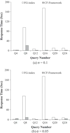
We measure the query response time with six types of queries (Q4, Q8, Q12, Q16, Q20 and Q24) when the size of the data is 10000. The query response time means the time to get the final answerDq given the queryq.Fig. 9shows the query response time according to the size of the query; the size of the query is the number of edges in the query (i.e., graph). We use the minimum frequency threshold
r
which is the parameter used for extracting frequent subgraphs. If jDfjPr
jDj;fis a frequent subgraph.Fig. 9(a) shows experiments whenr
is 0.1 andFig. 9(b) shows the experiments whenr
is 0.05. Whenr
is large, the number of features becomes small. We average the execution time for ten queries in each query set (Q-m).InFig. 9andFig. 9(b), in most cases, the CF-Framework shows a better performance than the FG-index in terms of the response time. The CF-Framework filters out the unnecessary graph data through two steps. Loose candidates are computed with a small cost using simple features while compact candidates are efficiently evaluated using graph features. Therefore, the CF-Framework can process various kinds of queries efficiently and shows a good performance in most cases as shown in Fig. 9. However, in the case of Q4, the CF-Framework has a worse performance than the FG-index. We will explain the reason for this in the following experiments. The query response time does not depend on only the size of the query as shown in
Fig. 7.Additional filtering algorithm.
The size of data 10000
The number of distinct labels 51 The number of vertices in each graph
Average: 25.4 Min: 2 Max: 214 The number of edges in each
graph
Average: 27.4 Min: 1 Max: 217 The number of distinct edges
in each graph
Average: 6.0 Min: 1 Max: 14
0 40 80 120 160 200 Q4 Q8 Q12 Q16 Q20 Q24
R
espo
n
se T
im
e
(Sec)
FG-index CF-Framework 0 40 80 120 160 200 Q4 Q8 Q12 Q16 Q20 Q24R
espo
n
se T
im
e
(Sec)
FG-index CF-Framework Query Number
Query Number
(a) =
σ
0.1
(b) =
σ
0.05
Fig. 9.Experiments according to the size of the query.
0 5 10 15 20 25 30 Q4 Q8 Q12 Q16 Q20 Q24
Re
spo
n
se
T
im
e
(Se
c)
FG-index CF-FrameworkQuery Number
Fig. 9. The FG-index shows a much worse performance in Q16 than that in other queries when compared to the CF-Framework.
In addition, we show the query response time inFig. 10when the size of data is small (the size of data = 2000,
r
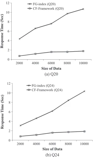
¼0:1). The result ofFig. 10shows a tendency similar to that ofFig. 9; therefore, we do not mention it in detail.Figs. 12–14show experiments according to the size of the data when
r
is 0.1. We conducted experiments on 2000, 4000, 6000, 8000, and 10,000 graph data. As we expected, the query response time increases for both the CF-Framework and the FG-index as the size of the data increases. Except for Q4 (Fig. 12(a)), the CF-Framework is superior to the FG-index.In the case of Q4, the number of edges in the query is small. Therefore, queries in Query Set Q4 may be contained in the index (i.e., FG-query). In the FG-index, if a query is an FG-query, the answer is returned without the candidate verification
Query FG-Query Size of
Result Q4 4 1930.5 Q8 0 194.4 Q12 0 23.1 Q16 0 7.8 Q20 0 1.9 Q24 0 0.4
Fig. 11.Characteristics of query sets.
(a) Q4
(b) Q8
0 0.5 1 1.5 2 2.5 3 2000 4000 6000 8000 10000 Respo n se T im e (Sec) FG-index (Q4) CF-Framework (Q4) 0 2 0 40 60 80 100 120R
espo
n
se T
im
e
(Sec)
FG-index (Q8) CF-Framework (Q8)Size of Data
2000 4000 6000 8000 10000Size of Data
and the FG-index shows a good performance in terms of the execution time.Fig. 11shows the number of FG-queries and the average size of results for each query set when the size of data is 10,000 and
r
is 0.1.Query Set Q4 contains four FG-queries (40%) and the resultant size is large compared to the other query sets. While the FG-index returns the result for the FG-queries in Query Set Q4 without verification, the CF-Framework should check whether a candidate is a real answer. Thus, for Q4, the CF-Framework has a worse performance than the FG-index. However, in most cases, queries are not FG-queries. Therefore, the CF-Framework can generally process various types of queries efficiently in comparison to the FG-index. It is not possible to index all subgraphs in order to returnDqwithout verification in the FG-index.
Fig. 15shows the query response time with respect to
r
. Asr
increases, the number of features becomes smaller. There-fore, the feature search time will be reduced. On the other hand, the size of the candidate answer will be larger since a small number of features are included in the query. There exists a trade-off between the feature search time and the time for the candidate verification. Thus, inFig. 15, the query processing time is not significantly affected byr
, and a particular tendency onr
is not shown.In addition, in order to compare the benefit for the first candidate set computation (using simple features) and the benefit for the second candidate set computation (using graph features), we conducted three experiments. One using only the first candidate set computation (‘‘First’’), one that only used the second candidate set computation (‘‘Second’’), and on that used both (‘‘First + Second’’) inFig. 16.Fig. 16shows the number of candidate answers for ‘‘First’’, ‘‘Second’’ and ‘‘First + Second’’. For ‘‘Second’’ and ‘‘First + Second’’, the number of candidate answers means the size ofCqPq(Cqis the candidate answer set andPqis the partial answer set) since we do not need to check the subgraph isomorphism for the partial answer set. ‘‘Sec-ond’’ is much more effective than ‘‘First’’ as shown inFig. 16since the second candidate set computation uses graph features. However, the second candidate set computation can be improved if it is integrated with the first candidate set computation. Therefore, ‘‘First + Second’’ shows the best performance in terms of the size of the candidate answer set. As the size of the query increases, the size of the candidate answer set decreases in both ‘‘First’’ and ‘‘Second’’. This is because the simple fea-ture value for a large-sized query is large and a large-sized query contains many graph feafea-tures.
(a) Q12
(b) Q16
0 2 4 6 8 2000 4000 6000 8000 10000Response Time (Sec)
FG-index (Q12) CF-Framework (Q12) 0 40 80 120 160 200 2000 4000 6000 8000 10000
Response Time (Sec)
FG-index (Q16) CF-Framework (Q16)
Size of Data
Size of Data
(a) Q20
(b) Q24
0 2 4 6 8 10 12 2000 4000 6000 8000 10000Respo
n
se T
im
e
(Sec)
FG-index (Q20) CF-Framework (Q20) 0 2 4 6 8 10 12 2000 4000 6000 8000 10000R
espo
n
se T
im
e
(Sec)
FG-index (Q24) CF-Framework (Q24)Size of Data
Size of Data
Fig. 14.Experiments according to the size of data (Q20, Q24).
0 40 80 120 160 200 Q4 Q8 Q12 Q16 Q20 Q24
Respo
n
se T
im
e
(Sec)
FG-index (0.05) CF-Framework (0.05) FG-index (0.10) CF-Framework (0.10) FG-index (0.15) CF-Framework (0.15) FG-index (0.20) CF-Framework (0.20)Query Number
Fig. 15.Experiments according tor.8. Conclusion
Recently, the large amount of graph data used in areas such as bio-informatics and social networks has been increasing. In those areas, the graph query problem is one of the most important, but subgraph isomorphism testing is an NP-complete problem. Therefore, to process a graph query efficiently, we propose a CF-Framework to retrieve graph data that contains the query. In the CF-Framework, we use two kinds of features: Simple features and graph features. Since simple features are easy to manage, the candidate set of the query is first retrieved using simple features. Then, using the graph features, which are difficult to manage but have better pruning power than the simple features, we can effectively reduce the size of the candidate set. Since it spends much time to find the graph features corresponding to the query, we propose an efficient graph-feature filtering algorithm called Cross Filtering, based on set properties. In Cross Filtering, by making two groups and filtering each group crossly, we can efficiently choose graph features that correspond to the query. The experimental results show that the CF-Framework can process various types of graph queries efficiently.
Acknowledgement
We would like to thank the editors and anonymous reviewers for their helpful comments. This work was supported by the National Research Foundation of Korea (NRF) Grant funded by the Korean Government (MSIP) (No. NRF-2014R1A1A2002499).
Appendix A. Examples for simple features A.1. Vertex count, edge count and max degree
We can useVertex Count, Edge Count, Max Degreeas basics. The Vertex Count is the number of vertices, Edge Count is the number of edges and Max Degree is the maximum degree among all vertices. For example, the Max Degrees forg1;g2;g3and
g4inFig. 1are 3, 2, 3, and 2, respectively. The values of the basic simple features are highly skewed. Therefore, the
discrim-inative power is low.
A.2. Vertex encoding and edge encoding
To exploit the property of the vertex and edge labels well, we use Vertex EncodingfVand Edge EncodingfEas simple fea-tures. Given graph datag¼ hVi;Ei;Li;lii, we encode the set of vertices (Vi) or edges (Ei) into thek-bit array. Assume two func-tionsf
v
:L! f0;1;. . .;k1gandfe:hL;L;Li ! f0;1;. . .;k1g, whereL¼ [iLi. Since the label of edgee¼ hv
1;v
2ican berepresented byhlð
v
1Þ;lðeÞ;lðv
2Þi, in this section, we uselðeÞas the meaning ofhlðv
1Þ;lðeÞ;lðv
2Þi. Usingfvandfe, we computethe vertex encoding value and the edge encoding value forViandEi, respectively. We assume thatMgandM0
garek-bit arrays to store vertex encoding value and edge encoding value for graphg, respectively, and are initialized as zero. For alla2V, we setMg½f
v
ðlðaÞÞto 1. Then,fVreturnsMg, which consists of thekbit array. In the same way, for alla2E, we setM0g½feðlðaÞÞto 1. The time complexity of computing the vertex encoding value isOðjVjÞand that of computing the edge encoding value is OðjEjÞ. Therefore, Vertex Encoding and Edge Encoding both have a small extraction time. In addition, to save the vertex encoding value and the edge encoding value, onlykbits are required for each encoding value. Finally, we should check the subgraph property offVandfE. We can defineas follows:
0 1000 2000 3000 4000 5000 6000 Q4 Q8 Q12 Q16 Q20 Q24
The number
of candidate answers
First Second First+SecondQuery Number
Fig. 16.The number of candidate answers.For the two-bit arraysMaandMb;MaMbiffMa&Mb¼Ma, where & is a bitwise AND operator.
Then,fV andfEsatisfy the subgraph property.
Proof. Prove that for any two graph data g1¼ hV1;E1;L1;l1iand g2¼ hV2;E2;L2;l2i, if g1g2, then fVðg1Þ fVðg2Þ and fEðg1Þ fEðg2Þ.
First, considerfVðg1Þ fVðg2Þ. We assume thatMg1 andMg2are k-bit arrays returned by the functionfV forg1andg2, respectively.
There are only two values inMg1½i. Case 1:Mg1½i ¼1.
IfMg1½i ¼1, thenMg2½i ¼1 (SinceV1V2).
Therefore,Mg1½i&Mg2½i ¼1.
Case 2:Mg1½i ¼0.
IfMg1½i ¼0, thenMg1½i&Mg2½i ¼0 regardless ofMg2½ivalue.
Therefore, by Case 1 and Case 2,Mg1½i&Mg2½i ¼Mg1½ifor any i. That is,fVðg1Þ fVðg2Þ. In the same way, we can prove thatfEðg1Þ fEðg2Þ. h
Example 4. We can extract the vertex encoding value forg1;g2;g3;g4andqusingfV as shown inFig. A.17. We extract the
vertex set from graph data and encode it by the function. We assume that k is 4 and the function is A?0, B?1, C?2, D?3, E?0 and F?1. SincefVðqÞ&fVðg1Þ ¼fVðqÞ;fVðqÞ fVðg1Þ. In the same way,fVðqÞ fVðg3Þ. Therefore,
g1andg3are candidates. Edge Encoding is processed like Vertex Encoding.
A B C
Graph Data
B B A Cg
1 A C Fg
3 A D D Cg
2 B A Bq
A B C E A C D A C F C C E C Eg
4 1 1 1 1 1 1 1 1 1 1 1 1 1 0 0 0 0 0 0 0References
[1] C. Chen, X. Yan, P.S. Yu, J. Han, D.-Q. Zhang, X. Gu, Towards graph containment search and indexing, in: International Conference on Very Large Data Bases (VLDB), 2007, pp. 926–937.
[2] J. Cheng, Y. Ke, W. Ng, A. Lu, Fg-index: towards verification-free query processing on graph databases, in: ACM SIGMOD International Conference on Management of Data, 2007, pp. 857–872.
[3]J. Cheng, Y. Ke, W. Ng, Efficient query processing on graph databases, ACM Trans. Database Syst. (TODS) 34 (1) (2009).
[4] C.-W. Chung, J.-K. Min, K. Shim, Apex: an adaptive path index for xml data, in: ACM SIGMOD International Conference on Management of Data, 2002, pp. 121–132.
[5] S.A. Cook, The complexity of theorem-proving procedures, in: ACM Symposium on Theory of Computing (STOC), 1971, pp. 151–158.
[6] B.F. Cooper, N. Sample, M.J. Franklin, G.R. Hjaltason, M. Shadmon, A fast index for semistructured data, in: International Conference on Very Large Data Bases (VLDB), 2001, pp. 341–350.
[7]A. Ferro, R. Giugno, M. Mongiovı`, A. Pulvirenti, D. Skripin, D. Shasha, Graphfind enhancing graph searching by low support data mining techniques, BMC Bioinformatics 9 (S-4) (2008).
[8] R. Giugno, D. Shasha, Graphgrep: a fast and universal method for querying graphs, in: International Conference on Pattern Recognition (ICPR), 2002, pp. 112–115.
[9] R. Goldman, J. Widom, Dataguides: enabling query formulation and optimization in semistructured databases, in: International Conference on Very Large Data Bases (VLDB), 1997, pp. 436–445.
[10]T.R. Hagadone, Molecular substructure similarity searching: efficient retrieval in two-dimensional structure databases, J. Chem. Inform. Comput. Sci. 32 (5) (1992) 515–521.
[11] H. He, A.K. Singh, Closure-tree: an index structure for graph queries, in: IEEE International Conference on Data Engineering (ICDE), 2006. [12]J. Huan, D. Bandyopadhyay, W. Wang, J. Snoeyink, J. Prins, A. Tropsha, Comparing graph representations of protein structure for mining family-specific
residue-based packing motifs, J. Comput. Biol. 12 (6) (2005) 657–671.
[13]W.-C. Hsu, I.-E. Liao, CIS-X: a compacted indexing scheme for efficient query evaluation of XML documents, Inform. Sci. 241 (2013) 195–211. [14] H. Jiang, H. Wang, P.S. Yu, S. Zhou, Gstring: a novel approach for efficient search in graph databases, in: IEEE International Conference on Data
Engineering (ICDE), 2007, pp. 566–575.
[15]U. Kang, M. Hebert, S. Park, Fast and scalable approximate spectral graph matching for correspondence problems, Inform. Sci. 220 (2013) 306–318. [16] R. Kaushik, P. Shenoy, P. Bohannon, E. Gudes, Exploiting local similarity for indexing paths in graph-structured data, in: IEEE International Conference
on Data Engineering (ICDE), 2002, pp. 129–140.
[17] A. Khan, Y. Wu, C.C. Aggarwal, X. Yan, NeMa: fast graph search with label similarity, in: International Conference on Very Large Data Bases (VLDB), 2013, pp. 181–192.
[18] C. Qun, A. Lim, K.W. Ong, D(k)-index: an adaptive structural summary for graph-structured data, in: ACM SIGMOD International Conference on Management of Data, 2003, pp. 134–144.
[19] P. Rao, B. Moon, Prix: indexing and querying xml using prüfer sequences, in: IEEE International Conference on Data Engineering (ICDE), 2004, pp. 288– 300.
[20] S. Sakr, Graphrel: a decomposition-based and selectivity-aware relational framework for processing sub-graph queries, in: International Conference on Database Systems for Advanced Applications (DASFAA), 2009.
[21] D. Shasha, J.T.-L. Wang, R. Giugno, Algorithmics and applications of tree and graph searching, in: ACM Symposium on Principles of Database Systems (PODS), 2002, pp. 39–52.
[22] Y. Tian, J.M. Pate, Tale: a tool for approximate large graph matching, in: IEEE International Conference on Data Engineering (ICDE), 2008. [23]G. Wang, B. Wang, X. Yang, G. Yu, Efficiently indexing large sparse graphs for similarity search, IEEE Trans. Knowl. Data Eng. (TKDE) 24 (3) (2012) 440–
451.
[24] H. Wang, S. Park, W. Fan, P.S. Yu, Vist: a dynamic index method for querying xml data by tree structures, in: ACM SIGMOD International Conference on Management of Data, 2003, pp. 110–121.
[25] X. Wang, X. Ding, A.K.H. Tung, S. Ying, H. Jin, An efficient graph indexing method, in: IEEE International Conference on Data Engineering (ICDE), 2012, pp. 210–221.
[26]P. Willett, J.M. Barnard, G.M. Downs, Chemical similarity searching, J. Chem. Inform. Comput. Sci. 38 (6) (1998) 983–996.
[27] D.W. Williams, J. Huan, W. Wang, Graph database indexing using structured graph decomposition, in: IEEE International Conference on Data Engineering (ICDE), 2007, pp. 976–985.
[28]L. Xu, T.W. Ling, H. Wu, Labeling dynamic XML documents: an order-centric approach, IEEE Trans. Knowl. Data Eng. 24 (1) (2012) 100–113. [29] X. Yan, P.S. Yu, J. Han, Graph indexing: a frequent structure-based approach, in: ACM SIGMOD International Conference on Management of Data, 2004,
pp. 335–346.
[30] X. Yan, P.S. Yu, J. Han, Substructure similarity search in graph databases, in: ACM SIGMOD International Conference on Management of Data, 2005, pp. 766–777.
[31] J. Yang, W. Jin, BR-Index: an indexing structure for subgraph matching in very large dynamic graphs, in: International Conference on Scientific and Statistical Database Management (SSDBM), 2011, pp. 322–331.
[32] D. Yuan, P. Mitra, H. Yu, C.L. Giles, Iterative graph feature mining for graph indexing, in: IEEE International Conference on Data Engineering (ICDE), 2012, pp. 198–209.
[33] Y. Yuan, G. Wang, H. Wang, L. Chen, Efficient subgraph search over large uncertain graphs, in: International Conference on Very Large Data Bases (VLDB), 2011, pp. 876–886.
[34] Y. Yuan, G. Wang, L. Chen, H. Wang, Efficient subgraph similarity search on large probabilistic graph databases, in: International Conference on Very Large Data Bases (VLDB), 2012, pp. 800–811.
[35] S. Zhang, S. Li, J. Yang, Gaddi: distance index based subgraph matching in biological networks, in: International Conference on Extending Database Technology (EDBT), 2009.
[36] S. Zhang, J. Yang, W. Ji, Sapper: subgraph indexing and approximate matching in large graphs, in: International Conference on Very Large Data Bases (VLDB), 2010, pp. 1185–1194.
[37] P. Zhao, J.X. Yu, P.S. Yu, Graph indexing: tree + deltaPgraph, in: International Conference on Very Large Data Bases (VLDB), 2007, pp. 938–949. [38] L. Zou, L. Chen, J.X. Yu, Y. Lu, A novel spectral coding in a large graph database, in: International Conference on Extending Database Technology (EDBT),
2008, pp. 181–192.
[39] Aids, <http://www.cs.ucsb.edu/xyan/software.htm>. [40] Datasets, <http://www.cs.ucsb.edu/xyan/software.htm>.