Divergence based classification in Learning Vector
Quantization
E. Mwebaze1,2, P. Schneider2,3, F.-M. Schleif4
, J.R. Aduwo1 , J.A. Quinn1 , S. Haase5 , T. Villmann5 , M. Biehl2
1 – Faculty of Computing & IT, Makerere University P.O. Box 7062, Kampala, Uganda
2 – Johann Bernoulli Institute for Mathematics and Computer Science, Univ. of Groningen P. O. Box 407, 9700AK Groningen, The Netherlands
3 – School of Clinical & Experimental Medicine, University of Birmingham, Birmingham, B15 2TT, UK
4 – CITEC, University of Bielefeld, Universit¨atsstr. 21-23, 33615 Bielefeld, Germany 5 – Department of MPI, University of Applied Sciences,
Technikumplatz 17, 09648 Mittweida, Germany
Abstract
We discuss the use of divergences in dissimilarity based classification. Diver-gences can be employed whenever vectorial data consists of non-negative, po-tentially normalized features. This is, for instance, the case in spectral data or histograms. In particular, we introduce and study Divergence Based Learning Vector Quantization (DLVQ). We derive cost function based DLVQ schemes for the family ofγ-divergences which includes the well-known Kullback-Leibler divergence and the so-called Cauchy-Schwarz divergence as special cases. The corresponding training schemes are applied to two different real world data sets. The first one, a benchmark data set (Wisconsin Breast Cancer) is available in the public domain. In the second problem, color histograms of leaf images are used to detect the presence of Cassava Mosaic Disease in cassava plants. We com-pare the use of standard Euclidean distances with DLVQ for different parameter settings. We show that DLVQ can yield superior classification accuracies and Receiver Operating Characteristics.
Keywords: classification, Learning Vector Quantization, prototype based classifiers, similarity measures, distance measures.
1. Introduction
Distance based classification schemes can be implemented efficiently in the framework of the popular Learning Vector Quantization (LVQ). LVQ systems are flexible, easy to implement, and can be applied in multi-class problems in a
straightforward fashion. Because LVQ prototypes are determined in the feature space of observed data, the resulting classifiers can be interpreted intuitively. Consequently, LVQ classifiers are widely used in a variety of areas including image processing tasks, medical applications, control of technical processes, or bioinformatics. An extensive bibliography including applications can be found in [1].
A key step in the design of any LVQ system is the choice of an appro-priate distance measure. Most frequently, practical prescriptions make use of Euclidean metrics or more general Minkowski measures, without further jus-tification. Generalized Euclidean measures and adaptive versions thereof have been introduced in the framework of relevance learning, see [2, 3, 4, 5, 6, 7] for examples.
Here, we explore an alternative class of distance measures which relates to approaches based on statistics or information theory. So-called divergences, for instance the most popular Kullback-Leibler divergence, quantify the dissimilar-ity of probabildissimilar-ity distributions or positive measures. They can immediately be employed as distances in supervised or unsupervised vector quantization, pro-vided the feature vectors and prototypes consist of non-negative, potentially normalized components. Note that throughout this article we use the terms distance anddistance measure in their general meaning, which does not imply symmetry or other metric properties.
Information theoretic distance measures have been discussed in the context of various machine learning frameworks, previously. This includes prototype based clustering, classification, or dimension reduction, see [8, 9, 10, 11, 12] for just a few recent examples. Frequently, divergences are employed to quantify the similarity of the prototype density with the observed distribution of data. Note that, here, we use divergences to quantify directly the distance between individual data points and prototype vectors. Moreover, we derive gradient based update schemes which exploit the differentiability of the divergences.
After setting up the general framework, we present the family of so-called
γ-divergences as a specific example. It is further specified by choice of a param-eterγand includes the well-known Kullback-Leibler and the so-called Cauchy-Schwarz divergence as special cases.
We develop the corresponding divergence based LVQ (DLVQ) schemes and apply them to two different classification problems. First, the Wisconsin Breast Cancer data set from the UCI data repository [13] is revisited. The second data set relates to the identification of the Casssava Mosaic Disease based on color histograms representing leaf images [14]. Performances are evaluated in terms of Receiver Operator Characteristics and compared with the standard LVQ scheme using Euclidean distance. The influence of the parameter γ is studied and we show that data set dependent optimal values can be identified.
In the next section we outline how divergences can be incorporated into the general framework of LVQ and we derive the corresponding gradient based training. In Sec. 3 we introduce the considered classification problems and data sets. Computer experiments are described and results are presented in Sec. 4, before we conclude with a summary and outlook.
2. Divergence based Learning Vector Quantization
For a particular classification task, we assume that a set of labeled example data is available:
{xµ, yµ}P
µ=1,
where thexµ∈IRN are feature vectors and the labelsyµ∈ {1,2, . . . C} specify
their class membership.
In an LVQ system we denote byW ={(wj, c(wj)} M
j=1a set ofM prototype
vectors wj ∈ IRN which carry labels c(wj) ∈ {1,2, . . . C}. Note that one or
several prototypes can be assigned to each class. Prototype vectors are identified in feature space and serve as typical representatives of their classes.
Together with a given distance measured(x,w), they parameterize the clas-sification scheme. Most frequently, aWinner-Takes-All scheme is applied: an arbitrary inputx is assigned to the class c(wL) of the closest prototype with d(x,wL)≤d(x,wj) for allj.
The purpose of training is the computation of suitable prototype vectors based on the available example data. The ultimate goal, of course, is general-ization: the successful application of the classifier to novel, unseen data. LVQ training can follow heuristic ideas as in Kohonen’s original LVQ1 [15]. A va-riety of modifications has been suggested in the literature, aiming at better convergence or favorable generalization behavior. A prominent and appealing example is the cost function based Generalized Learning Vector Quantization (GLVQ) [16]. We will resort to the latter as an example framework in which to introduce and discuss divergence based LVQ. We would like to point out, how-ever, that differentiable divergences could be incorporated into a large variety of cost-function based or heuristic training prescriptions.
GLVQ training is guided by the optimization of a cost function of the form
E(W) = P X µ=1 Φ d(xµ,w J)−d(xµ,wK) d(xµ,wJ) +d(xµ,wK) , (1)
wherewJ denotes the closest correct prototype withc(wJ) =yµandwK is the
closest incorrect prototype (c(wK)6=yµ). Note that the argument of Φ in Eq.
(1) is restricted to the interval [−1,+1]. While Φ is in general a non-linear (e.g. sigmoidal) function [16], we consider here the simple case Φ(x) =x.
In principle, a variety of numerical optimization procedures is available for the minimization of the cost function (1). On-line training using stochastic gradient descent is a particularly simple method which has proven useful in many practical applications. In stochastic gradient descent, a single, randomly selected examplexis presented and the corresponding winnerswJ,wK are up-dated incrementally by ∆wJ= −η dK(x) (dJ(x) +dK(x))2 ∂ ∂wJdJ(x) , ∆wK = +η dJ(x) (dJ(x) +dK(x))2 ∂ ∂wKdK(x) (2)
wheredL(x) =d(x,wL) and∂/∂wL denotes the gradient with respect to wL. The learning rateηcontrols the step size of the algorithm. Training is performed in so-called epochs, each of which presents all examples in the training data in a randomized order.
Practical prescriptions are obtained by inserting a specific distanced(x,w) and its gradient. Meaningful dissimilarities should satisfy the conditions
d(x,w)≥0 for all x,w and d(x,w) = 0 for w=x.
Note that the LVQ framework does not require that the distance measure sat-isfies metric properties such as triangular inequalities or symmetry. In both, training and working phase, only distances between data and prototype vec-tors have to be evaluated, the distances between two prototypes or two feature vectors are never used.
In the following we assume that the data consists of vectors of non-negative componentsxj ≥0 which are normalized toPN
j=1xj= 1. Potential extensions
to non-normalized positive data are discussed at the end of this section. Normalized non-negative xj can be interpreted as probabilities. This in-terpretation may be just formal, as for instance in the first example data set (WBC) that we consider in the following section. Probabilistic interpretations appear natural in many cases, for instance, whenever the vectors x represent histograms or spectra. An important example for the former is the character-ization of images by normalized gray value or color histograms, which we also consider in our second example data set, see Sec. 3. Frequently, spectral data is conveniently normalized to constant total intensity and is employed for classifi-cation in a large variety of fields including remote sensing or bioinformatics [1]. Assuming normalized non-negative data suggests, of course, the consideration of prototype vectors which satisfy the same constraints. Hence, we enforce
wj≥0 and
N
X
j=1
wj= 1 (3)
explicitly after each training step, Eq. (2).
Under the above assumptions, information theory provides a multitude of potentially useful dissimilarity measures. Different classes of divergences and their mathematical properties are detailed in [17, 18], while [19] presents first examples of Divergence Based LVQ.
We compare results of DLVQ with the standard choice, i.e. (squared) Eu-clidean distance: Deu(x,w) = 1 2(x−w) 2 , ∂Deu(x,w) ∂ wk =−(xk−wk). (4)
Inserting the derivative with respect towinto the general framework leads to the familiar GLVQ algorithm which moves the updated prototypes either towards or away from the presented feature vector, depending on their class labels [16].
Our first results concern the so-called Cauchy-Schwarz (CS) divergence, as introduced in [20]: Dcs(x,w) = 1 2log x2w2 −logxTw, ∂Dcs(x,w) ∂ wk = wk w2− xk xTw. (5)
It is particularly simple and, like the Euclidean measure, obeys the symmetry relationd(x,w) =d(w,x).
It might be interesting to note that, apart from the logarithm, the CS-measure is formally identical to the Pearson Correlation [21] in the case of zero mean data. Pearson Correlation has been used in the context of LVQ, see [21]. However, it is important to realize that the CS-divergence is applied only to non-negative and, consequently, non-zero mean data.
In the following, we extend our preliminary studies of the CS-divergence [19] and consider the more general family ofγ-divergences, see [17, 18] for the mathematical background: Dγ(y,z) = 1 γ+ 1 log X j yγ+1j 1 γ · X j zjγ+1 −log X j yjzjγ 1 γ (6) fory,z∈IRN. The precise form of this dissimilarity measure is controlled by
the parameterγ >0. Note that forγ = 1 one obtains the symmetric Cauchy-Schwarz divergence as a special case, while the limitγ →0 yields the popular Kullback-Leibler divergence.
In general, for γ6= 1, dγ(x,y)6=dγ(y,x). The asymmetry is also reflected in the derivatives with respect to the first or second argument, respectively. Consequently, the use of d(x,w) = Dγ(x,w) yields a DLVQ scheme different from the one derived ford(x,w) =Dγ(w,x).
In the following we consider only training processes which make consistent use of either Dγ(w,x) or Dγ(x,w), respectively. One and the same measure is employed throughout the entire training process and when evaluating the classification performance. Accordingly, one of the following derivatives has to be inserted into Eq. (2) to yield the actual DLVQ prescription[17, 18]:
∂ Dγ(w,x) ∂ wj = 1 γ wγj P k w γ+1 k − 1 γ xγj P k wkx γ k (7) ∂ Dγ(x,w) ∂ wj = wγj P k w γ+1 k − xjw γ−1 j P k xkw γ k . (8)
Note thatγ-divergences withγ >0 are invariant under rescaling of the argu-ments: Dγ(λy, µz) =Dγ(y,z) for λ, µ >0 [17, 18]. Hence, the normalization of the feature vectors,P
jxj = 1, is not required in the formalism and has no
effect on the results presented here. This invariance does not hold for more general dissimilarities, as discussed in [17].
3. Data sets and classification problems
Two different real world data sets serve as a testbed for the suggested DLVQ algorithms.
3.1. Wisconsin Breast Cancer (WBC) Data
We first apply DLVQ to a popular benchmark problem: The Wisconsin Breast Cancer (original) data set (WBC) from the UCI data repository [13]. Disregarding 16 vectors which contain missing values, the WBC set provides 683 examples in 9 dimensions. The data contains labels corresponding to ma-lignant(239 examples) andbenignsamples (444 examples). Single features cor-respond to different score values between 1 and 10, see [13] for their definition. This does not imply a natural interpretation of feature vectors as histograms or probabilities. However, the application of the divergence based formalism is possible and it is justified to the same degree as the more popular choice of Euclidean distances. For a more detailed description of this data set and further references we refer the reader to [13] and [22]. We apply a normalization such thatP
jxj = 1 for the following analysis.
3.2. Cassava Mosaic Disease (CMD) Data
The second data set corresponds to features extracted from leaf images of cassava plants as provided by the Namulonge National Crops Resources Re-search Institute, Uganda. Sample images represent 92 healthy plants and 101 plants infected with the cassava mosaic disease. For example images and further details of the image acquisition see [14].
Standard processing techniques were employed to remove background and clutter and in order to obtain a set of characteristic features from the leaf images. When aiming at optimal classification performance, various sets of features may be taken into account [14]. Here we limit the analysis to the aspect of discolorization caused by the disease. For the application of DLVQ we consider normalized histograms with 50 bins representing the distribution of hue values in the corresponding image. Example hue histograms can also be found in [14]. The application of DLVQ appears natural in this problem, as the information is represented by normalized histograms reflecting statistical properties of the data.
4. Computer experiments and results
For the following evaluation and comparison of algorithms, we split the avail-able data randomly into training (90% of the data) and test set (10%). If not stated otherwise, all results reported in the following were obtained as averages over 25 randomized splits. In both cases, we consider the simplest possible LVQ system with one prototype per class, only. Their initial positions are obtained as the mean of 50% randomly selected examples from each class in the respective training set.
The effect of the learning rate on performance depends on properties of the data set and on the distance measure in use. For simplicity, training is performed at constant learning rates in this first study. In order to facilitate a fair comparison, we determined a close to optimal learning rate from preliminary runs with respect to the achieved accuracies after a fixed number of training epochs. For each algorithm we selected the best learning rate from the set
10−3,10−4, . . . ,10−12 . Results presented in the following are obtained after
200 training epochs for the WBC data and after 1500 epochs with CMD data. The learning rates employed for the WBC data set wereη = 10−4 when using
Euclidean distances and η = 10−6 for γ-divergences. In the CMD data set,
learning rates of η = 10−5 (Euclidean measure) and η = 10−6 (γ-divergences)
have been used.
After training we determine training and test set accuracies of the classifiers and we report the average values obtained over the validation runs. When comparing classifiers, it is important to take into account that greater overall test accuracies do not necessarily indicate better performance. The Winner-Takes-All LVQ classifier represents just one working point, i.e. one combination of class 1 error and class 2 error. In particular, for unbalanced data sets a more detailed evaluation of the classification performance is instrumental.
In order to obtain further insight, we introduce a biasθto the classification rule after training: an input vectorxis assigned to class 1 if
d(x,w1)< d(x,w2) +θ, (9) wherewi is the closest prototype representing classi. The bias of the resulting
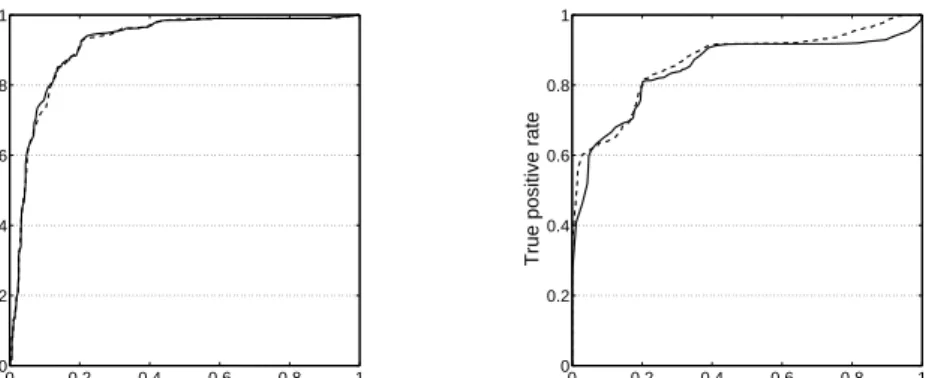
classification towards one of the classes depends on the sign and magnitude of the threshold. By varyingθ, the full Receiver Operating Characteristics (ROC) of the classifier can be obtained [23, 24]. Results presented in Figure 1 display a threshold-average over the validation runs [24]. In the ROC,false positive rates correspond to the fraction of truly benign cases (WBC data) or healthy plants (CMD) which are misclassified. Correspondingly, thetrue positive rategives the rate at which truly malignant (WBC) or diseased plants (cassava) are correctly classified. As an important and frequently employed measure of performance we also determine the corresponding area under curve (AUC) with respect to training set and test set performance.
4.1. Euclidean Distance and Cauchy-Schwarz Divergence
We first compare the two symmetric distance measures discussed here: stan-dard Euclidean metrics and the Cauchy-Schwarz divergence. Figure 1 displays the ROC with respect to test set performances in the WBC benchmark problem (left panel) and the CMD data set (right panel).
Table 1 summarize numerical findings in terms of the observed training and test accuracies for the unbiased LVQ classifier withθ= 0 and the AUC of the Receiver Operator Characteristics.
Note that for the WBC (original) data set, higher accuracies have been reported in the literature, see [13] for references. Here, we consider only the
WBC training acc. test acc. AUC (training) AUC (test)
Deu(x,w) 0.850 (0.040) 0.845 (0.041) 0.924 (0.004) 0.918 (0.004)
Dcs(x,w) 0.864 (0.003) 0.853 (0.007) 0.923 (0.005) 0.916 (0.005)
CMD training acc. test acc. AUC (training) AUC (test)
Deu(x,w) 0.790 (0.005) 0.782 (0.007) 0.856 (0.006) 0.848 (0.007)
Dcs(x,w) 0.807 (.0002) 0.805 (.0004) 0.872 (0.003) 0.867 (0.003)
Table 1: Numerical results for WBC and CMD data sets: mean accuracies in the unbiased LVQ classifier and AUC with respect to training and test sets, respectively. Numbers in parentheses give the standard deviation as observed over the validation runs.
simplest LVQ setting in order to compare the use of Euclidean and divergence based distance measures. The optimization of the DLVQ performance and the comparison with competing methods will be addressed in forthcoming studies.
In the WBC problem we do not observe drastic performance differences be-tween the considered distance measures. The Cauchy-Schwarz based DLVQ scheme does outperform standard Euclidean LVQ in the CMD data set as sig-naled by the greater AUC values. This reflects the fact that the CMD data set contains genuine histograms, for which the use of DLVQ seems natural. 4.2. The family ofγ-Divergences
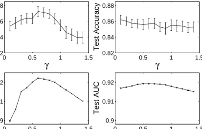
The precise form of the γ-divergence is specified by the parameterγ >0 in Eq. 6. In addition, we can select the measureDγ(x,w) orDγ(w,x), respectively. We display the mean test set accuracies as well as the AUC of the ROC as functions ofγ for both variants of theγ-divergence in Fig. 2 (WBC data) and in Fig. 3 (CMD).
In both data sets we do observe a dependence of the AUC performance on the value of γ with a more or less pronounced optimum in a particular choice of the parameter. This is not necessarily paralleled by a maximum of the corresponding test set accuracy for unbiased LVQ classification as the latter represents only one particular working point of the ROC.
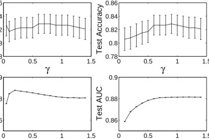
Note that in the range of values γ displayed in Fig. 3 (right panel), corre-sponding to the use ofDγ(w,x), the AUC appears to saturate for large values of the parameter. Additional experiments, however, show that performance decreases weakly whenγ is increased further.
WBC γ AUC (test) Dγ(x,w) 0.6 0.922 (0.004) Dγ(w,x) 0.5 0.919 (0.005) CMD γ AUC (test) Dγ(x,w) 0.2 0.888 (0.003) Dγ(w,x) 1.2 0.882 (0.004)
Table 2: Best performance in terms of the mean test set AUC and corresponding value ofγ
for the WBC and CMD data sets. Values in parenthesis correspond to the observed standard deviations.
0 0.2 0.4 0.6 0.8 1 0 0.2 0.4 0.6 0.8 1
False positive rate
True positive rate
0 0.2 0.4 0.6 0.8 1 0 0.2 0.4 0.6 0.8 1
False positive rate
True positive rate
Figure 1: ROC curves for the WBC data set (left panel) and CMD data set (right panel). For the WBC data, results are shown on average over 100 randomized training set compositions, whereas for the CMD data we have performed 200 randomized runs. In both cases, the ROC curves were threshold-averaged [24]. Results are displayed for the GLVQ variants based on Euclidean distances (solid lines) and Cauchy-Schwarz divergence (dashed lines).
For both data sets, the influence of γ appears to be stronger and the best achievable AUC is slightly larger in the DLVQ variant usingDγ(x,w). Table 2 summarizes numerical results in terms of the best observed test set AUC and the corresponding values ofγas found for WBC and CMD data in both variants of theγ-divergence.
5. Summary and Conclusion
We have presented DLVQ as a novel framework for distance based classifi-cation. The use of divergences as distance measures is, in principle, possible for all data sets that contain non-negative feature values. It appears particularly suitable for the classification of histograms, spectra, or similar data structures for which divergences have been designed, originally.
As a specific example for this versatile framework we have considered the family ofγ-divergences which contains the so-called Cauchy-Schwarz divergence as a special case and approaches the well-known Kullback-Leibler divergence in the limitγ→0. We would like to point out that a large variety of differentiable measures could be employed analogously, an overview of suitable divergences is given in [17, 18].
The aim of this work is to demonstrate the potential usefulness of the approach. To this end, we considered two example data sets. The Wiscon-sin Breast Cancer (original) data is available from the UCI Machine Learning Repository [13] and serves as a popular benchmark problem for two-class classi-fication. The second data set comprises histograms which represent leaf images for the purpose of the detection of the Cassava Mosaic Disease [14].
In case of the WBC data we observe little differences in performance quality when comparing standard Euclidean metrics based LVQ with DLVQ employing
0 0.5 1 1.5 0.82 0.84 0.86 0.88
γ
Test Accuracy 0 0.5 1 1.5 0.9 0.91 0.92γ
Test AUC 0 0.5 1 1.5 0.82 0.84 0.86 0.88γ
Test Accuracy 0 0.5 1 1.5 0.9 0.91 0.92γ
Test AUCFigure 2: Overall test set accuracies for the unbiased LVQ system withθ= 0 (upper panels) and AUC of the ROC (lower panels) as a function ofγfor the WBC data set. The left panel displays results for the distanceDγ(x,w), while the right panel corresponds to the use of
Dγ(w,x). Error bars mark the observed standard errors of mean.
the Cauchy-Schwarz divergence. When using the more generalγ-divergences, a weak dependency onγ is found which seems to allow for improving the perfor-mance slightly by choosing the parameter appropriately.
In contrast to the WBC, the CMD data set consists of genuine histogram data and the use of divergences appears more natural. In fact, we find improve-ment over the standard Euclidean measure already for the symmetric Cauchy-Schwarz divergence. Further improvement can be achieved by choosing an ap-propriate value ofγ in both variants of the non-symmetric distance measure. The dependence onγ and its optimal choice is found to be data set specific.
The application of DLVQ appears most promising for problems that involve data with a natural interpretation as probabilities or positive measures. In forthcoming projects we will address more such data sets. Potential applications include image classification based on histograms, supervised learning tasks in a medical context, or the analysis of spectral data as in bioinformatics or remote sensing.
Besides the more extensive study of practical applications, future research will also address several theoretical and conceptual issues. The use of diver-gences is not restricted to the GLVQ formulation we have discussed here, it is possible to introduce DLVQ in a much broader context of heuristic or cost func-tion based LVQ algorithms. Within several families of divergences it appears feasible to employ hyperparameter learning in order to determine, for instance,
0 0.5 1 1.5 0.78 0.8 0.82 0.84 0.86
γ
Test Accuracy 0 0.5 1 1.5 0.86 0.88 0.9γ
Test AUC 0 0.5 1 1.5 0.78 0.8 0.82 0.84 0.86γ
Test Accuracy 0 0.5 1 1.5 0.86 0.88 0.9γ
Test AUCFigure 3: Same as Figure 2, but here for the CMD data set. The left panel corresponds to the use ofDγ(w,x), while results displayed in the right panel were obtained forDγ(w,x).
the optimalγ directly in the training process, see [25] for a similar problem in the context of Robust Soft LVQ [26]. The use of asymmetric distance measures raises interesting questions concerning the interpretability of the LVQ proto-types, we will address this issue in forthcoming projects, as well.
Finally, the incorporation of relevance learning [2, 3, 4, 5, 6] into the DLVQ framework is possible for measures that are invariant under rescaling of the data, such as theγ-divergences investigated here. Relevance learning in DLVQ bears the promise to yield very powerful LVQ training schemes.
Acknowledgment: Frank-Michael Schleif was supported by the Federal Min-istry of Education and Research, Germany, FZ: 0313833, and the German Re-search Foundation (DFG) in the projectRelevance Learning for Temporal Neu-ral Maps under project code HA2719/4-1. Ernest Mwebaze was supported by The Netherlands Organization for International Cooperation in Higher Ed-ucation (NUFFIC), Project NPT-UGA-238: Strengthening ICT Training and Research Capacity in Uganda.
References
[1] Neural Networks Research Centre. Bibliography on the
self-organizing map (SOM) and learning vector quantiza-tion (LVQ). Helsinki, University of Technology, available at: http://liinwww.ira.uka.de/bibliography/Neural/SOM.LVQ.html, 2002.
[2] T. Bojer, B. Hammer, D. Schunk, and K. Tluk von Toschanowitz. Rel-evance determination in Learning Vector Quantization. In M. Verleysen, editor, Proc. of Europ. Symp. on Art. Neural Networks (ESANN), pages 271–276. d-side, 2001.
[3] B. Hammer and T. Villmann. Generalized relevance learning vector quan-tization. Neural Networks, 15(8-9):1059–1068, 2002.
[4] P. Schneider, M. Biehl, and B. Hammer. Adaptive relevance matrices in learning vector quantization. Neural Computation, 21:3532–3561, 2009. [5] P. Schneider, M. Biehl, and B. Hammer. Distance learning in discriminative
vector quantization. Neural Computation, 21:2942–2969, 2009.
[6] P. Schneider, K. Bunte, H. Stiekema, B. Hammer, T. Villmann, and M. Biehl. Regularization in matrix relevance learning. IEEE Trans. on Neural Networks, 21(5):831–840, 2010.
[7] K. Bunte, B. Hammer, A. Wism¨uller, and M. Biehl. Adaptive local dis-similarity measures for discriminative dimension reduction of labeled data. Neurocomputing, 73(7–9):1074–1092, 2010.
[8] E. Jang, C. Fyfe, and H. Ko. Bregman divergences and the self organis-ing map. In C. Fyfe, D. Kim, S.-Y. Lee, and H.Yin, editors, Intelligent Data Engineering and Automated Learning IDEAL 2008, pages 452–458. Springer Lecture Notes in Computer Science 5323, 2008.
[9] A. Banerjee, S. Merugu, I. Dhillon, and J. Ghosh. Clustering with Bregman divergences. Journal of Machine Learning Research, 6:1705–1749, 2005. [10] T. Villmann, B. Hammer, F.-M. Schleif, W. Herrmann, and M. Cottrell.
Fuzzy classification using information theoretic learning vector quantiza-tion. Neurocomputing, 71:3070–3076, 2008.
[11] K. Torrkola. Feature extraction by non-parametric mutual infromation maximization. Journal of Machine Learning Research, 3:1415–1438, 2003. [12] K. Bunte, B. Hammer, T. Villmann, M. Biehl, and A. Wism¨uller. Ex-ploratory observation machine (XOM) with Kullback-Leibler divergence for dimensionality reduction and visualization. In M. Verleysen, editor, European Symposium on Artificial Neural Networks (ESANN 2010), pages 87–92. d-side publishing, 2010.
[13] D.J. Newman, S. Hettich, C.L. Blake, and C.J. Merz. UCI reposi-tory of machine learning databases. Irvine, CA: University of Cali-fornia, Department of Information and Computer Science, available at: http://www.ics.uci.edu/ mlearn/MLRepository.html, 1998.
[14] J.R. Aduwo, E. Mwebaze, and J.A. Quinn. Automated vision-based diag-nosis of cassava mosaic disease. In P. Perner, editor,Industrial Conference on Data Mining - Workshops, pages 114–122. IBaI Publishing, 2010.
[15] T. Kohonen. Self-Organizing Maps. Springer, Berlin, 2nd edition, 1997. [16] A. S. Sato and K. Yamada. Generalized learning vector quantization. In
Advances in Neural Information Processing Systems, volume 8, pages 423– 429, 1996.
[17] T. Villmann and S. Haase. Mathematical aspects of divergence based vector quantization using frechet-derivatives. Technical Report MLR-03-2009, Univ. Leipzig/Germany, 2009. ISSN:1865-3960 http://www.uni-leipzig.de/˜compint/.
[18] T. Villmann, S. Haase, F.-M. Schleif, B. Hammer, and M. Biehl. The mathematics of divergence based online learning in Vector Quantization. In Proc. Fourth International Workshop on Artificial Neural Networks in Pat-tern Recognition (ANNPR 2010), volume 5998 of Springer Lecture Notes in Artificial Intelligence LNAI, pages 108–119. Springer, 2010.
[19] E. Mwebaze, P. Schneider, F.-M. Schleif, S. Haase, T. Villmann, and M. Biehl. Divergence based learning vector quantization. In M. Verleysen, editor, Proc. of the 18th European Symp. on Artificial Neural Networks (ESANN), pages 247–252. d-side publishing, 2010.
[20] J.C. Principe, J.F. III, and D. Xu. Information theoretic learning. In S. Haykin, editor, Unsupervised Adaptive Filtering. Wiley, 2000.
[21] M. Strickert, U. Seiffert, N. Streenivasulu, W. Weschke, T. Villmann, and B. Hammer. Generalized relevance LVQ (GRLVQ) with correlation mea-sures for gene expression analysis. Neurocomputing, 69(7–9):651–659, 2006. [22] K.P. Bennett and O.L. Mangasarian. Robust linear programming discrimi-nation of two linearly inseparable sets.Optimization Methods and Software, 1:23–34, 1992.
[23] R. O. Duda, P. E. Hart, and D. G. Stork. Pattern Classification (2nd Edition). Wiley-Interscience, 2000.
[24] T. Fawcett. An introduction to ROC analysis.Patt. Rec. Lett., 27:861–874, 2006.
[25] P. Schneider, M. Biehl, and B. Hammer. Hyperparameter learning in proba-bilistic prototype-based models.Neurocomputing, 73(7–9):1117–1124, 2010. [26] S. Seo and K. Obermayer. Soft learning vector quantization. Neural