Improved Multi-Task Learning Based on Local Rademacher Analysis

(1)

University of Central Florida University of Central Florida

STARS

Electronic Theses and Dissertations, 2004-2019

2017

Improved Multi-Task Learning Based on Local Rademacher

Analysis

Niloofar Yousefi

University of Central Florida

Part of the Industrial Engineering Commons

Find similar works at: https://stars.library.ucf.edu/etd University of Central Florida Libraries http://library.ucf.edu

This Doctoral Dissertation (Open Access) is brought to you for free and open access by STARS. It has been accepted for inclusion in Electronic Theses and Dissertations, 2004-2019 by an authorized administrator of STARS. For more information, please contact [email protected].

STARS Citation STARS Citation

Yousefi, Niloofar, "Improved Multi-Task Learning Based on Local Rademacher Analysis" (2017). Electronic Theses and Dissertations, 2004-2019. 5544.

(2)

IMPROVED MULTI-TASK LEARNING BASED ON LOCAL RADEMACHER ANALYSIS

by

NILOOFAR YOUSEFI

B.S. Iran University of Science & Technology, 2008 M.S. University of Tehran, 2012

A dissertation submitted in partial fulfilment of the requirements for the degree of Doctoral of Philosophy

in the Department of Industrial Engineering and Management Systems in the College of Engineering and Computer Science

at the University of Central Florida Orlando, Florida

Summer Term 2017

(3)

c

(4)

ABSTRACT

Considering a single prediction task at a time is the most commonly paradigm in machine learn-ing practice. This methodology, however, ignores the potentially relevant information that might be available in other related tasks in the same domain. This becomes even more critical where facing the lack of a sufficient amount of data in a prediction task of an individual subject may lead to deteriorated generalization performance. In such cases, learning multiple related tasks to-gether might offer a better performance by allowing tasks to leverage information from each other. Multi-Task Learning (MTL) is a machine learning framework, which learns multiple related tasks simultaneously to overcome data scarcity limitations of Single Task Learning (STL), and there-fore, it results in an improved performance. Although MTL has been actively investigated by the machine learning community, there are only a few studies examining the theoretical justification of this learning framework. The focus of previous studies is on providing learning guarantees in the form of generalization error bounds. The study of generalization bounds is considered as an important problem in machine learning, and, more specifically, in statistical learning theory. This importance is twofold: (1) generalization bounds provide an upper-tail confidence interval for the true risk of a learning algorithm the latter of which cannot be precisely calculated due to its de-pendency to some unknown distributionP from which the data are drawn, (2) this type of bounds can also be employed as model selection tools, which lead to identifying more accurate learning models.

The generalization error bounds are typically expressed in terms of the empirical risk of the learn-ing hypothesis along with a complexity measure of that hypothesis. Although different complexity measures can be used in deriving error bounds, Rademacher complexity has received considerable attention in recent years, due to its superiority to other complexity measures. In fact, Rademacher complexity can potentially lead to tighter error bounds compared to the ones obtained by other

(5)

complexity measures. However, one shortcoming of the general notion of Rademacher complex-ity is that it provides a global complexcomplex-ity estimate of the learning hypothesis space, which does not take into consideration the fact that learning algorithms, by design, select functions belonging to a more favorable subset of this space and, therefore, they yield better performing models than the worst case. To overcome the limitation of global Rademacher complexity, a more nuanced notion of Rademacher complexity, the so-called local Rademacher complexity, has been consid-ered, which leads to sharper learning bounds, and as such, compared to its global counterpart, guarantees faster convergence rates in terms of number of samples. Also, considering the fact that locally-derived bounds are expected to be tighter than globally-derived ones, they can motivate better (more accurate) model selection algorithms.

While the previous MTL studies provide generalization bounds based on some other complex-ity measures, in this dissertation, we prove excess risk bounds for some popular kernel-based MTL hypothesis spaces based on the Local Rademacher Complexity (LRC) of those hypotheses. We show that these local bounds have faster convergence rates compared to the previous Global Rademacher Complexity (GRC)-based bounds. We then use our LRC-based MTL bounds to de-sign a new kernel-based MTL model, which enjoys strong learning guarantees. Moreover, we develop an optimization algorithm to solve our new MTL formulation. Finally, we run simulations on experimental data that compare our MTL model to some classical Multi-Task Multiple Kernel Learning (MT-MKL) models designed based on the GRCs. Since the local Rademacher complexi-ties are expected to be tighter than the global ones, our new model is also expected to exhibit better performance compared to the GRC-based models.

(6)

(7)

ACKNOWLEDGMENTS

In the past five years, I was very fortunate to receive support and help from many people, and I would like to take this opportunity to thank these individuals in writing.

First and foremost, I would like to thank my committee chair Prof. Mansooreh Mollaghasemi for giving me guidance and support. I am deeply grateful for having had the opportunity to be her Ph.D. student. I am especially thankful for the wonderful example she has provided as a successful woman, mentor, instructor and advisor.

I am also greatly indebted to my advisor Prof. Michael Georgiopoulos for creating the inspiring and creative research environment, in which I have performed my graduate studies. His ultimate willingness to invest himself into the guidance and support of young scientists and researchers, his ability to inspire his students and encourage them to stay engaged and focused on learning are unrivaled. His personality, patience, motivation, enthusiasm and dedication make him a great mentor, advisor, and more importantly a role model. I especially thank him for providing guidance at key moments during my research at the Machine Learning Lab (ML2_{) at University of Central}

Florida.

My deep appreciation goes to my co-advisor Prof. Georgios Anagnostopoulos for his invaluable guidance and feedback on my research and for always being available to advise me. I would like to thank Dr. Anagnostopoulos for spending an enormous amount of time for our extensive and valuable discussions on various machine learning as well as mathematical problems. I would never forget the numerous discussions we had, which made my Ph.D productive and stimulating. This thesis owes its existence to his support and caring mentoring during various stages of my Ph.D. tenure.

(8)

I would also like to sincerely thank my other committee members, Dr. Luis Rabelo, Dr. Qipeng Zheng and Dr. Petros Xanthopoulos for devoting time to assess my research work, and providing valuable suggestions and comments through this process.

Moreover, I want to thank present and past members of the ML2for all the chats and good memo-ries we shared during the stressful and difficult moments of our Ph.D endeavor.

Besides mentors, this dissertation is greatly influenced by the contribution of Prof. Marius Kloft who has given me tremendous help during the completion of this investigation. I would like to express my sincere appreciation and gratitude to Dr. Kloft for his invaluable and inspiring sug-gestions and sharing his vast knowledge and experience with me, which helped gaining a deeper understanding of statistical learning theory.

A very special thank goes to my parents for their unflagging love, faith and encouragement in all my pursuits. My greatest fortune is being blessed with a family that has been always supportive and encouraging even when it meant traveling thousand of miles to pursue life on a different continent. I appreciate their unconditional support that gives me freedom to explore the world.

Most importantly, I would like to thank my best friend, soul-mate, and husband, Ali who has been a true and great supporter. I would like to express my heartfelt appreciation for being by my side throughout my Ph.D. studies even during the most difficult times. His faith in me, quiet patience and unwavering love kept my spirits up and encouraged me to embark on this journey.

Finally, I acknowledge financial support from National Science Foundation (NSF) grant No. 1161228 (COMPASS Project), and No. 1200566 (AEGIS RET Program). Any opinions, findings, and con-clusions or recommendations expressed in this material are those of the authors and do not neces-sarily reflect the views of the NSF.

(9)

LIST OF TABLES

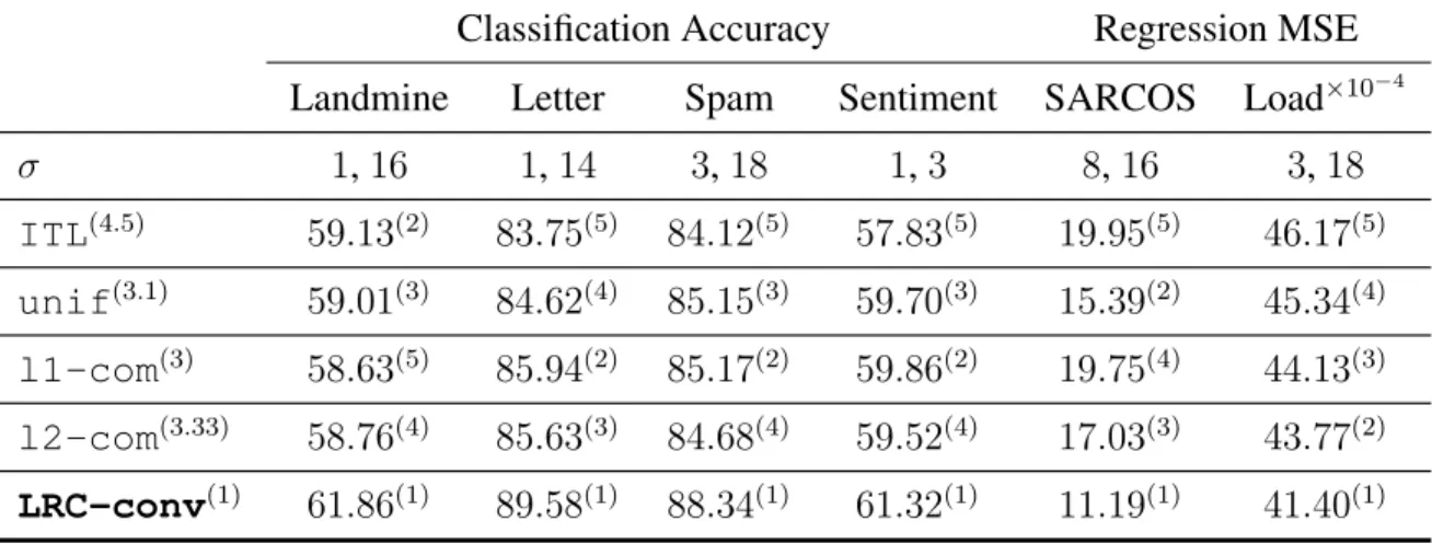
Table 7.1: Experimental comparison between LRC-conv and four other methods on six benchmark datasets. The superscript next to each model indicates its rank. The best performing algorithm gets rank of1. . . 104

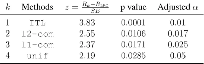
Table 7.2: Comparison of ourLRC-convmethod against the other methods with Holm’s test . . . 105

(15)

CHAPTER 1: INTRODUCTION

Introduction

While most traditional machine learning approaches focus on the learning of a single independent task at a time, Multi-Task Learning (MTL), in contrast, aims to training several related tasks to-gether, with the hope of improving the overall performance of all tasks by allowing information sharing between them. More specially, when only a limited number of training samples per each task exists, MTL can benefit tasks by inducing a positive inductive bias in the learning process of multiple related tasks. Therefore, more effective training can be conducted in this way, which leads to improved generalization performance for each task compared to the “no transfer” scenario, where each task is learned in isolation.

Nowadays, MTL frameworks are routinely employed in a variety of settings. Some application domains include computer vision [1, 60, 79, 122, 137, 149], HIV therapy screening [15], collabo-rative filtering [22], age estimation from facial images [149], and sub-cellular location prediction [142] , Information retrieval [121, 22, 123], bioinformatics [15, 142, 90] and finance [52] just to name a few prominent ones.

The underlying assumption behind the MTL paradigm is based on tasks’ relatedness. Therefore, the key concern of MTL is “how to capture tasks relatedness and integrate it into the learning formulation.” In response to this question, several MTL approaches have been designed, which employ different strategies to capture task relatedness. Although, these models differ in how they model the relationship among tasks, they mostly formulate MTL as a regularized Empirical Risk Minimization (ERM) problem, in which the objective function is a composition of an over-the-tasks average error and a regularization term to encourage information sharing among over-the-tasks in

(16)

some capacity. More precisely, similar to many machine learning models, the regularized MTL formulation is typically given as

min

f L(f) +λΩ(f) (1.1)

wheref is a vector-valued function that consists of the tasks’ learning functions(f1, . . . , fT),L(f)

is the averaged empirical loss over all tasks, andΩ(f)is the regularization term which is designed to enforce information sharing among tasks. Also,λis the regularization parameter that allows for choosing the right trade-off betweenL(f)andΩ(f). There are many prior efforts which utilize this framework to model task relationships, among which we refer to [47, 155, 158, 129, 103, 102], just to name a few. It is worth pointing out that in some cases, instead of (or besides) the regularization term, some optimization constraints are also incorporated into MTL formulation (1.1) in favor of adding some other desired characteristics. A good example of this situation is where a clustering or grouping strategy is needed to be considered in order to allow different level of information sharing between different tasks. This goal can then be achieved by imposing clustering-type constraints into Problem (1.1). Also, in order to allow more flexibility and achieve better generalization per-formance, kernel-based regularizations have been proposed in the context of MTL [46]. Beside flexibility, simplicity and generality of kernels and their associated Reproducing Kernel Hilbert Space (RKHS)s, “availability of effective error bounds and stability analysis relative to perturba-tions of the data” [109] is another attractive feature of kernel-based regularizers. Interestingly, it can be shown that there is an equivalency (Ivanov-Tikhonov regularization equivalency) between (1.1) and optimization problem

min

f L(f)

(17)

which can be efficiently used to identify the hypothesis space of the learning problem at hand. In more detail, givenT learning tasks, the learning problem 1.2 seeks the vector-valued function

f = (f1, . . . , fT)from the hypothesis spaceF :={f = (f1, . . . , fT) : Ω(f) ≤ R}such that the

average empirical errorL(f)is minimized.

Problem Statement

The study of generalization error bounds is important in machine learning problems, as they are uniform over the learning hypothesis space, that is, the bounds hold for any functionf within the hypothesis space under consideration. These type of bounds provide upper-tail confidence intervals for the true risk. But, even more importantly, the same bounds can also be used as model selection tools where, among several alternatives, one can identify the model that most likely has the lowest risk. In particular, such a bound is usually based on an empirical measurement of its risk (error) and a measure of its complexity. Also, it is worth pointing out that

To be more concrete regarding the importance of the generalization bounds, recall that the main goal of any typical machine learning algorithm is to automate the process of learning a model based on some observations from a phenomenon in order to make good predictions in the future with the help of the learned model [21]. To make this more precise, consider a supervised learn-ing paradigm (as we restrict ourselves to this case in this dissertation), and n training samples

{(X1, Y1), . . . ,(Xn, Yn)}, which are identically and independently drawn from an unknown

distri-bution P. A supervised learning algorithm then, aims to construct a function f :X → Y, which depends on this observed data and generalizes well over any unseen future data (X, Y). Hence, the goal is to select a function f ∈ F with small risk or expected loss _E(X,Y)∼P [`(f(X), Y)].

However, the calculation of this quantity is impossible, as the distribution P is unknown. One common approach to estimate the true risk_E(X,Y)∼P[`(f(X), Y)]is to relate this quantity by its

(18)

empirical counterpart along with a complexity measure of the function classF. A typical form of a generalization bound is E(X,Y)∼P[`(f(X), Y)]≤ 1 n n X i=1

`(f(Xi), Yi) +h(complexity of the function classF, n) (1.3)

It is worth mentioning that different complexity measures such as Vapnik-Chevonenkis (VC) dimension, fat-shattering dimension or covering numbers can be used in deriving generaliza-tion bounds. However, in this dissertageneraliza-tion, we use a more recent nogeneraliza-tion of complexity called Rademacher complexity, which, in turn, can be bounded by other complexity measures (such as covering numbers or VC dimension), and therefore improves existing bounds based on these other measures. More importantly, the generalization bounds based on empirical version of the Rademacher complexity are data dependent, meaning that they measure the complexity of the function class F based on the training samples. In other words, these data-dependent general-ization bounds can be estimated based on finite samples and they are usually tighter than their distribution-dependent counterparts [111]. Also, data-dependent bounds (such as Rademacher-based bounds) are of more value as they can provide strong theoretical foundation in designing of new learning algorithms. As an example, for kernel-based hypotheses, the empirical Rademacher-based bounds are typically functions of the kernel matrix. This can lead to deriving kernel learning algorithms which, by considering a regularization on the trace of the kernels, benefits from strong learning guarantees. As an effective complexity measure, the Rademacher complexity was first proposed by [74], [9] and [107]. However, one shortcoming of the general notion of Rademacher complexity is that it provides the global estimation of the complexity of the function classF. In other words, it does not take into consideration the fact that learning algorithms, typically, pick functions belonging to a more favorable subset of the function class, and they therefore yield bet-ter performance than the worst case. Recall that most learning algorithms tend to choose functions

(19)

inducing small empirical errors and also (hopefully) small generalization errors. Therefore, it is very likely that the function fˆ∈ F minimizing the empirical risk 1_nPn

i=1`(f(Xi), Yi), lies in a

neighborhood of the best function f∗ ∈ F that minimizes the true risk _E(X,Y)[`(f(X), Y)]. To

overcome the limitation of global Rademacher complexity, a finer notion of Rademacher com-plexity, the so-called local Rademacher complexity, has been considered which leads to sharper learning bounds and as such also (compared to its global counterpart, i.e. GRC) guarantees a faster rate of convergence—the rate at which the empirical risk approaches the true risk—under some general conditions. Also, regarding the fact that local bounds are expected to be tighter than the global ones, they can motivate more efficient model selection algorithms.

The idea of LRC is to restrict the function classF to a mush smaller subset of it, by imposing a variance-type constraint on this class of functions. Since such a small class can also have smaller Rademacher complexity, they can lead to sharper bounds compared to GRC-based bounds.

Contributions

Although MTL has been actively investigated by the machine learning community, there are only a few studies examining the theoretical perspective of this learning framework. While these previous MTL studies provide generalization bounds based on some other complexity measures such as covering number and VC-dimension [11, 13, 2] or GRC [101, 102, 104, 105] of the learning hypothesis, we are not aware of any study taking advantage of the LRCs to derive error bounds for MTL. In this dissertation, we derive excess risk bounds for some popular kernel-based MTL hypothesis spaces based on the LRC of those hypotheses. It turns out that similar to the STL scenario, for kernel-based hypotheses, the data-dependent LRC-based MTL bounds are functions of the tail sum of the eigenvalues of the kernel matrices. Also, as expected (and it has been shown for STL [10]), we show that theses local bounds have faster convergence rate compared

(20)

to previously known GRC-based bounds. Furthermore, similar to what has been done in [38] for STL, we use our LRC-based MTL bounds to design a kernel-based MTL model which considers a constraint based on the tail sum of the eigenvalues of the kernels. Finally, we show that our new LRC-based MTL model consistently outperforms the traditional kernel learning algorithms, whose performances have been proven to be difficult to surpass in the past; such as uniform combination solution as well as convex combination of base kernels. Note that it can be shown that the latter case—with an`1 norm constraint on kernel parameter—corresponds to a model which is derived

based on a GRC analysis. We show the superiority of our LRC model against this GRC-based algorithm, by performing a series of experiments.

Organization

The rest of this dissertation is organized as follows: In Chapter 2, we provide some background on statistical learning theory, and some of its concepts including supervised learning, generaliza-tion error bounds, global and local Rademacher complexity-based bounds. Finally, we introduce the general MTL setting and formulation at the end of Chapter 2. Chapter 3 presents a literature review associated with MTL models and generalization bounds. Also, the methodology of our study can be found in Chapter 4. Then, Chapter 5 details the derivation of the LRC-based gener-alization bound for MTL. Risk bounds are eventually found for several common MTL framework considering norm regularizers. A thorough analysis of the derived bound as well as an insightful comparison to the existing bounds is included which demonstrates the advantages of the LRC-based bounds. Additionally, due to the superiority of the derived LRC bounds, a new kernel-LRC-based MTL model along with an optimization algorithm are introduced in Chapter 6. The experimental evaluation of the work is given in Chapter 7. Chapter 8 provides summary and potential future directions of the work.

(21)

CHAPTER 2: BACKGROUND

With the ever-increasing amount of data, it is almost impossible for a human programmer or spe-cialist to detect a meaningful pattern in data and translate it to some expertise or knowledge for the future use. For this reason,machine leaning, as an automated learning tool, has become a central part of human life over the past couple of decades. Machine learning refers to an automated process of detecting meaningful patterns from data, and it has applications in many real world problems where information extraction from large data sets is required. Ranking the relevant web pages given a submitted query into a search engine, filtering email messages by an anti-spam software, securing credit card transactions by a fraud detection software, detecting faces in digital photos, recognizing voice commands on smart phones, and accident preventing systems in cars are just some examples of machine learning applications in real world problems. Machine learning also appears in many other scientific guises such as bioinformatics, medicine, and astronomy. In this section, we provide some background on the main concepts underlying machine learning.

Automated Learning

Learning, of course, covers a wide range of processes which is difficult to define precisely. Conse-quently, machine learning has waded into several branches, each of which dealing with a different type of learning task. However, the common feature of all different types of machine learning models is that they automate the process of an inductive inference including, observing a phe-nomenon, building a model based on the observed phephe-nomenon, and making predictions using the constructed model.

(22)

learning, and primarily, we will be dealing with binary classification problems. In this framework, the phenomenon is defined as some instance-label pairs, where a label is either +1 or −1. A classification model is then constructed as a mapping function from the instances to the labels. This function is expected to make future predictions for unseen instances with as few mistakes as possible. Note that it is always possible to build a function that agrees very well with the observed (training) data. However such a model might exhibit a poor performance in predicting unseen future data. As example of this instance is the case where the training data are noisy. This phenomenon is referred to asoverfitting, and it happens when the model can fit the training data too well. This type of models are usually too complex in the sense that they have too many free parameters to tune. Therefore, one way to avoid overfitting is to restrict the choice of the learning model to a set of predictors with less complexity. This set of predictors is called a hypothesis class and it is typically chosen in advance based on some specific assumptions or knowledge about the data. Another way to avoid overfitting is to add a penalty (to the learning process) for complicated hypothesis classes. This is usually referred to asregularizationtechnique, and it is known as a very successful method in all machine learning problems. By using one of these (and usually the combination of both) techniques, we can expect that the learning model can be reasonably generalized from the observed data to future unseen instances. In other words, the model is expected to make future predictions with as small risk as possible. In the following, we discuss in more detail: “What isregularizationtechnique?”, “How to quantify thecomplexityof a hypothesis class?”, or“ How to measure thegeneralizationof a model?”. Before answering these fundamental questions, let us first to formally describe the supervised learning paradigm.

(23)

Formalization

Consider an input space X as the set of objects we want to label. Also, assume that the output spaceY denotes the set of possible labels, which are chosen as{−1,+1}for binary classification. We then assume that the training data{(X1, Y1), . . . ,(Xn, Yn)}are identically and independently

drawn from an unknown distribution P defined on X × Y. Now, given the training data, the objective of a learning algorithm is to choose a function f : X → Y among the functions in the hypothesis class F, which generalizes well. In other words, this function should be chosen in such a way that the probability of error P(f(X) 6= Y)is small for any unseen instance pair (X, Y)∈ X × Y. Therefore, thetrue riskof a predictor functionf can be given as

R(f) :=_E(X,Y)∼P [(f(X)6=Y)] = E 1f(X)6=Y . (2.1) Regularization

The objective of a learning algorithm is to choose a function f ∈ F that minimizes the risk

R(f). However, the true riskR(f) cannot be calculated, due to its dependency to the unknown distributionP. But, we can quantify the consistency of the functionfwith the training data through anempirical riskdefined as

Rn(f) := 1 n n X i=1 1f(Xi)6=Yi. (2.2)

which is commonly used as a criterion to choose a functionf from the hypothesis spaceF. This algorithm, which is calledEmpirical Risk Minimization, is based on the idea of choosing a predic-tor functionf ∈ Fwhich minimized (2.2). However, as mentioned earlier, this hypothesis classF

(24)

to enlargeF as much as possible to increase the chances of finding a good predictorf inF. From the other side, enlargingF might increase the risk of overfitting. Therefore, a regularizer is usually imposed on F to prevent overfitting, while choosing a large classF. Intuitively, the regulariza-tion funcregulariza-tion Ω(f) is a measure of the complexity ofF that reflects some prior belief about the problem. Regularized empirical risk minimization algorithms solve the following problem

min f∈F 1 n n X i=1 1f(Xi)6=Yi+λΩ(f) (2.3)

which tries to balance between “better fit” and “less complexity” ofF.

Generalization Error Bounds

In a binary classification setting, given a predictor functionf : X → _R, by convention, the point

X is considered to be classified as class +1 if f(X) > 0, and class −1if f(X) < 0, and it is considered misclassified otherwise. In other words, any instance(Xi, Yi)is classified correctly by

the predictor functionf, only ifYif(Xi) >0. Therefore, the risk associated to functionf can be

defined as

E1Y f(X)≤0

where1Y f(X)≤0 is known as0−1loss, and it is a non-convex, non-differentiable function. These

characteristics make the optimization hard. For this reason, a convex or/and differentiable surro-gate function`, which upper-bounds this loss, is optimized. For ease of notation, letZi := (Xi, Yi)

andZ := (X, Y). Now we define the class oflossfunctionLF associated withf as

(25)

Also, for convenience, let us introduce the shorthand notationsP `f :=E(X,Y)∼P [`(f(X), Y)]and

Pn`f := 1_n

Pn

i=1`(f(Xi), Yi)as the true and empirical risks off, respectively.

As noted earlier, the optimal goal is to characterize the true risk associated with the predictor functionf. However, as it depends on the unknown probabilityP, it is impossible to estimate this quantity. One way to approximate the true risk R(f) is to relate it to its empirical counterpart, and one prominent approach to do this is based on the theory of uniform convergence of empirical quantities to their mean (see e.g. [140]). In other words, this theory provides an upper-bound on the quantity

P `f −Pn`f (2.4)

It it worth pointing that the bound on (2.4) is usually expressed as a function of the complexity of

F along with a function of the number of samples n. An important aspect of the generalization bounds is that they are uniform over the learning hypothesis spaceF, that is, these bounds hold for any functionf which lies within the function classF. Although, different complexity measures can be used in deriving generalization bounds, in this dissertation, we use a more recent notion of complexity calledRademacher complexity, which usually leads to tighter, high-quality bounds.

Relationship of Error Bounds to Empirical Processes

This section provides some insights on how the generalization error bounds can be obtained. Recall that in order to find the generalization bounds, one needs to obtain bounds onP f−Pnf, in which

the functionf is chosen from a function spaceF := {f : X × Y → _R}. As mentioned before, this quantity is a random variable, and the randomness stems from (i) the unknown distributionP

(26)

function fromF [20]. However, the latter randomness can be removed by considering a collection of random variablesP f −Pnf indexed by the function setF:

{P f −Pnf}_f∈F, (2.5)

which is known as the empirical process in statistical learning theory. A more helpful quantity associated to an empirical process is

sup

f∈F

(P f −Pnf). (2.6)

Note that a bound on (2.6) also acts a bound on (2.5). Since the supremum of the empirical process

P f−Pnfin (2.6) is still random due to its dependency on the unknown distributionP, the bounds

for this quantity takes the probabilistic form

P sup f∈F (P f −Pnf)≥x ≤δ, (2.7)

where δ > 0. The expression in (2.7) is usually referred to as concentration inequality which provides a bound on the probability that a random variableZ differs from its expected value_EZ

by more than a certain amount. A number of methods have been proposed to derive these type of inequalities such as martingale methods [110, 106], decoupling methods [41], Talagrand’s induc-tion method [133, 134, 93, 115] and the so-called “entropy method” which is based on logarithmic Sobolev inequalities introduced in [80, 81, 16, 125, 100, 94, 17, 19, 19]. Being related to the tail bounds of empirical processes, we are interested to obtain probabilistic bounds for{Z−_EZ ≥x}, in whichZ :=Pn

i=1Xi, whereX1, . . . , Xnarenindependent random variables. One useful bound

of this form is the so-called Hoeffding’s tail inequality which is introduced bellow.

(27)

variables such that for eachi ∈ 1, . . . , n, Xi takes values in[ai, bi]. IfZ :=

Pn

i=1, Xi , then for

anyx >0, the following holds

P{Z−EZ ≥x} ≤exp ₋ 2x2 Pn i(bi−ai)2 and, P{Z−EZ ≤ −x} ≤exp ₋ 2x2 Pn i(bi−ai)2

The generalization of Hoeffding’s inequality to functions of i.i.d. random variables is know as McDiarmid (or bounded differences) inequality.

Theorem 2(McDiarmid’s Inequality). For functiong :Xn _→

R, letZ :=g(X1, . . . , Xi, . . . , Xn)

andZi :=g(X1, . . . , Xi−1, Xi0, Xi+1, . . . , Xn). Assume that for allX1, . . . , Xn, X10, . . . , X

0

n ∈ Xn,

and for alli∈ {1, . . . , n},

|Z−Zi| ≤ci.

Then, for anyx >0,

P{|Z−EZ|> x} ≤2 exp −2x2 Pn i=1c2i

One limitation of Hoeffding type inequalities, however, is that they ignore the information about the variance of the Xis. Note that in many cases the variance of Z might be mush smaller than

Pn

i=1c2i. For this reason, sharper bounds such as Bennett’s and Bernstein’s inequalities have been

(28)

such that for alli={1, . . . , n},_E[Xi] = 0, andV ar[Xi] :=σ2. IfZ :=

Pn

i=1Xi, and there exist

a constantc >0such thatXi ≤c, then for anyx >0, we have

P{Z−EZ ≥σ

√

2nx+cx 3 } ≤e

−x

The functional version of Bernstein’s inequality applicable to function classes has been also pro-posed which is known as Talagrand’s inequality. In the following, we introduce Bousquet’s version of Talagrand’s inequality presented in [19].

Theorem 4 (Talagrand’s Concentration Inequality). Assume that for function class F := {f :

X →_R}, it holds that_Ef(Xi) = 0,∀i, andsupf∈F, X∈X f(X)≤1. Let Z := sup f∈F n X i f(Xi), andsup_f_∈F _n1 Pn i=1f(Xi)≤σ

2_{with the real number}_{σ >}_{0. Then, for any}_{x >}_{0, we have}

P{Z−EZ ≥ √ 2xν+x 3} ≤e −x whereν:=nσ2_{+ 2} EZ.

Now based on these McDiarmid’s and Talagrand’s inequalities, we can derive such inequalities for the suprema of empirical processes. For this purpose, one can easily defineZ := sup_f_∈F(P f −

Pnf)for which we obtain the following results.

(29)

classFmapX ∈ X into[0,1]. McDiarmid inequality then gives, with probability at least1−e−x_, sup f∈F P f −Pnf ≤E sup f∈F P f −Pnf + r 2x n

Corollary 6(Talagrand’s Inequality for the Suprema of Empirical Processes). LetF be a class of functions mappingX ∈ X into[0,1]. Assume thatris a positive real value for whichV ar[f(Xi)]≤

rfor allf ∈ F. Then, for everyx >0, with probability at least1−e−x_,

sup f∈F P f −Pnf ≤2E sup f∈F P f −Pnf + r 2xr n + 4x 3n

As you can see, the term _Esup_f_∈FP f −Pnf

is one of the main components of the bound in both inequalities above. Thanks to the symmetrization technique, this term can be also bounded based on the fact that for any functionsf inF, the expected deviation of the empirical meanPnf

from its true oneP f, can be controlled by the Rademacher complexity of the function classF.

Lemma 1(Symmetrization Technique, Lemma A.5 in [10]). For any function classF

max E sup f∈F P f −Pnf ,_E sup f∈F Pnf −P f ≤2R(F).

R(F)is the so-calledRademacher complexityof the function class F which will be discussed in the next section.

Rademacher Complexity

Rademacher complexity quantifies how well the functions in a hypothesis class G can correlate with random noise, and therefore it measures the richness of the hypothesis setG. In the following,

(30)

we provide the definition and some useful property of the Rademacher complexity which will be used in the future chapters.

Definition 7(Rademacher Complexity). Given a hypothesis classG :={g :Z → _R}and a set of dataS :={z1, . . . zn}which are drawn identically and independently according to distributionP,

the Empirical Rademacher Complexity ofGis defined as

ˆ R(G) :=_Eσ ( sup g∈G 1 n n X i=1 σig(zi) )

whereσis are independent uniformly-distributed{±1}-valued random variables. Also, the Rademacher

Complexity of G is defined as the expectation of the empirical Rademacher complexity over all samples of sizendrawn according toP:

R(G) :=_ES∼Pn

h ˆ R(G)i.

Intuitively, for a fixed set S and a fixed Rademacher vector σ := {σ1, . . . , σn}, the supremum

measures the maximum correlation betweeng(zi)andσi over all functionsg ∈ G. Therefore, by

taking the expectations over the random vectorσ, the empirical Rademacher complexity measures how well, on average, the functions g ∈ G can be correlated with random noise over the fixed sample setS. Also, Rademacher complexity measures the expected noise-fitting ability ofG over anyrandomsample set of sizendrawn according toPn.

The following Talagrand lemma provides a useful property for the Rademacher Complexity. Using this property, the Rademacher complexity of a hypothesis spaceF after composition with a Lips-chitz functionφ can be upper-bounded in terms of the Rademacher complexity of the hypothesis setF.

(31)

that is,|φ(x)−φ(y)| ≤L|x−y|. Then for every function classF there holds

EσR(φ◦ F)≤LEσR(F), (2.8)

whereφ◦ F :={φ◦f :f ∈ F }and◦is the composition operator.

In the following section we introduce some fundamental theorems providing generalization bound based on the Rademacher Complexity.

Rademacher Complexity-based Generalization Bounds

The following theorem, which is based on McDiarmid’s inequality, serves as a general tool for providing generalization bounds based on Rademacher complexity.

Theorem 8 (Rademacher complexity-based generalization bound for general function class F, Theorem 3.1 in [112]). Let G be a family of functions mapping from Z to [0,1]. Assume that

S :={z1, . . . , zn}is a set ofnsamples which are drawn identically and independently according

to the probability distribution D. Then for any g ∈ G and x > 0, the following holds with probability at least1−e−x_, E[g(z)]≤ 1 n n X i=1 g(zi) + 2R(G) + r x 2n, E[g(z)]≤ 1 n n X i=1 g(zi) + 2 ˆR(G) + r 9x 2n

whereR(G)andRˆ(G)are Rademchar and empirical Rademacher complexities ofG.

(32)

Theorem 9(Rademacher complexity-based generalization bound for binary classification, Theo-rem 3.2 in [112]). Let LF := {`f : (X, Y)→`(f(X), Y), f ∈ F } be a class of loss functions

with ranges in [0,1]. Assume that the function classF is a set of functions f : X → _R, and

{(X1, Y1), . . . ,(Xn, Yn)}is a set ofnsamples distributed identically and independently according

toP. Also let the loss function`be anL-Lipschitz, and upper-bound the0−1loss function. Fix

L >0, then for anyf ∈ F andx >0, with probability at least1−e−x_,

E[`(f(X), Y)]≤ 1 n n X i=1 `(f(Xi), Yi) + 2LR(F) + r x 2n, E[`(f(X), Y)]≤ 1 n n X i=1 `(f(Xi), Yi) + 2LRˆ(F) + r 9x 2n

whereR(F)andRˆ(F)are Rademchar and empirical Rademacher complexities ofF.

Note that the first term in the right-hand side of the above inequalities is the empirical risk of func-tionf, and the second term is a measure of complexity of hypothesis classF. Based on this obser-vation, it is not hard to see that these error bounds can be used to design complexity-regularization algorithms, similar to (2.3), for model selection. These type of algorithm are usually of interest, as they minimize the upper bound on the true risk _E[`(f(X), Y)], hence a better generalization performance is expected by utilizing them as learning algorithms. Also, it can be seen that the best error rate that can be achieved using global Rademacher complexity is at least of the order of

O(1/√n).

The derivations of these bounds are based on the application of McDiarmid’s inequality which is the functional version of Hoeffding’s inequality, and it does not use any information regarding the variance of the functions. For this reason, another type of functional inequality, namely Talagrand’s inequality, has been used in the derivation of generalization bounds. Talagrand’s inequality is based on Bernstein’s concentration inequality and yields sharper bounds by incorporating additional data

(33)

on the variances of the functions into the derivations. Talagrand’s inequality was first established in [132] and later improved by [82, 100, 125, 19]. The following section presents a generalization bound based on Talagrand’s inequality, which requires a new definition of Rademacher complexity, namely thelocalRademacher complexity.

Local Rademacher Complexity-based Generalization Bounds

local Rademacher complexity refers to the Rademacher complexity of a subset of the function classF which is determined by a variance constraint on the functions in that class.

Definition 10(Local Rademacher Complexity (LRC)). Given a hypothesis classG :={g : Z →

R}, and a set of dataS := {z1, . . . zn}which are drawn identically and independently according

to distributionP, the empirical local Rademacher complexity of the function classGat radiusris defined as ˆ R(G, r) := _Eσ      sup g∈G, P g2≤r 1 n n X i=1 σig(zi)     

whereσi’s are independent random variables uniformly chosen from{±1}. Also, the local Rademacher

Complexity ofG is defined as the expectation of the empirical local Rademacher complexity over all samples of sizendrawn according toP:

R(G, r) :=_ES∼Pn

h ˆ

R(G, r)i.

The reason for the definition of local Rademacher complexity is based on the fact that by incorpo-rating the variance constraint better error rate for the bounds can be obtained. In other words, the

(34)

mizes the true risk), the variance of the deviation between the empirical and true errors of functions can be controlled by a linear function of the expectation of this difference. Based on this obser-vation, instead of considering the Rademacher complexity of the entire class, we can consider the Rademacher complexity of a subset of the class which is usually the intersection of the class with a ball centered at the best functionf∗in the class [10]. Note that local Rademacher complexity is always smaller than its corresponding global one, as it considers a smaller subset of the class.

Before presenting the localized version of error bounds, first we introduce some concepts and definition which are used later in this section and also in the future chapters for the derivation of local generalization bounds.

Definition 11(Sub-Root Function). A functionψ : [0,∞]→[0,∞]is sub-root if

1. ψis non-negative,

2. ψis non-decreasing,

3. r7→ψ(r)/√ris non-increasing forr >0.

The following lemma is an immediate consequence of the above definition.

Lemma 3(Lemma 3.2 [10]). Assume thatψ is a sub-root function. Then one can show thatψ is continuous on[0,∞], and the equationψ(r) =rhas a unique (non-zero) solution which is known as the fixed point ofψ and it is denotes byr∗. Moreover, for anyr > 0, it holds thatr > ψ(r)if and only ifr∗ ≤r.

The following provides another useful definition that will be needed in introducing the main result of this section.

(35)

Definition 12(Star-Hull). The star-hull of a function classF around the functionf0is given as

star(F, f0) :={f0+α(f −f0) :f ∈ F, α ∈[0,1]}

Now, we present a lemma from [21] which indicates that the local Rademacher complexity of the star-hull of any function classF can be considered as a sub-root function, and it has a unique fixed point. We will see later that this fixed point plays a key role in the local error bounds.

Lemma 4 (Lemma 6 in [21]). For any function classF, the local Rademacher complexity of its start-hull is a sub-root function.

Now, we can state the main results of this section as the following theorem which is a consequence of Talagrand’s inequality.

Theorem 13(Local Rademacher complexity-based generalization bound for general function class

F, Theorem 3.3 in [10]). LetF be a class of functions satisfyingsup_x|f(x)| ≤b. Let{Xi}ni=1be

a sequence ofnrandom variables which are independently and identically distributed according to

P. Assume that there exist a constantBand a functionV :F →_R+_{such that for every}_f _{∈ F}_{, it}

holds thatP f2 _≤_V₍_f₎_≤_{BP f}_{, where}_{P f}2 _:=

EX∼P[(f(X))2]and similarlyP f :=EX∼Pf(X).

Letψ be a sub-root function with the fixed pointr∗. Suppose that

BR(F, r)≤ψ(r),∀r ≥r∗,

whereR(F, r)is the LRC of the function classF defined as

R(F, r) :=_EX,σ      sup f∈F, P f2_≤_r 1 n n X i=1 σif(xi)     

(36)

Then for anyf ∈ F,K >1andx >0, with probability at least1−e−x_, P f ≤ K K−1Pnf + 704K B r ∗ +(22b+ 26BK)x n . wherePnf := _n1 Pn i=1f(Xi).

Also, ifF is a convex class of functions, and for any α ∈ [0,1], V(αf) ≤ α2_V₍_f_{), then for any}

f ∈ F,K >1andx >0the following inequality holds with probability at least1−e−x,

P f ≤ K K−1Pnf + 6K B r ∗ +(22b+ 5BK)x n .

Now, it can be shown (as we see later in Section 5 of Chapter 5), considering additional conditions on the data distribution P or on the hypothesis setF, can make an improvement on the (excess) risk bounds in term of the convergence rate. These assumptions are presented in the following.

Assumption 14. Consider the loss function`and the function classF which satisfy the following conditions

1. For every probability distributionP, there exists a functionf ∈ F, which satisfiesP `f∗ = inff∈FP `f.

2. There is a constantB >1, such that for everyf ∈ F, we haveP(f−f∗)≤BP(`f −`f∗). 3. There exists a constantL, such that the loss function`( ˆY , Y)isL-Lipschitz in its first

argu-ment, that is for anyY,Yˆ1,Yˆ2,

|`( ˆY1, Y)−`( ˆY2, Y)| ≤L|Yˆ1−Yˆ2|.

(37)

used regularized ERM algorithms. With the help of Assumption 14 and Theorem 13, the following theorem presents an excess risk bound of the function classF.

Theorem 15 (Distribution-dependent local Rademacher complexity-based excess risk bound for binary classification, Corollary 5.3 in [10]). Assume that F is a class of functions satisfying sup_x|f(x)| ≤ 1. Also, let (Xi, Yi)ni=1 be a sequence of n independent random variables

dis-tributed according toP. Suppose that Assumption 14 holds. DefineF∗ _:=_{_f ₋_f∗_}_{, where} _f∗ _is the function satisfyingP `f∗ = inf_f_∈FP `_f. Also, letfˆ∈ F be such thatP_n`_ˆ

f = inff∈FPn`f.

As-sume thatψis a sub-root function with the fixed pointr∗ such thatBLR(F∗_{, r}₎_≤_ψ₍_r_),_∀_r_≥_r∗_, whereR(F∗_{, r}₎_{is the LRC of the function class}_F∗_{, and it is defined as}

R(F∗_{, r}_{) :=} EX,σ sup f∈F, P(f−f∗₎_≤_r 1 n n X i=1 σif(Xi) .

Then for anyf ∈ F,K >1,x >0andψ(r)≤r, with probability at least1−e−x,

P(`_fˆ−`f∗)≤ 704K B r ∗ +(11L+ 26BK)x n . whereP(`_fˆ−`f∗) :=_E_X_∼_P`( ˆf(X), Y)−`(f∗(X), Y).

Also, if F is a convex class of functions, then for any f ∈ F, K > 1and x > 0, the following inequality holds with probability at least1−e−x,

P(`_fˆ−`f∗)≤ 6K B r ∗ + (11L+ 5BK)x n . (2.9)

The result of Theorem 15 uses a distribution-dependent measure of complexity of the function class

F. In other words, the sub-root functionψin Theorem 15 is bounded in terms of the Rademacher averages that cannot be computed without knowing the probability distributionP. The next

(38)

the-orem, analogous to Corollary 5.4 in [10], presents a data-dependent version of (5.9) replacing the Rademacher complexity in Theorem 15 with its empirical counterpart. Indeed, this error bound can be directly computed from the data, without having a priori information of the distribution.

Theorem 16 (Data-dependent local Rademacher complexity-based excess risk bound for binary

classification, Corollary 5.4 in [10]). Assume that F is a convex class of functions satisfying sup_x|f(x)| ≤ 1. Also, let (Xi, Yi)ni=1 be a sequence of n independent random variables

dis-tributed according to P. Suppose that Assumption 14 holds. Also, let fˆ ∈ F be such that

Pn`_fˆ= inff∈FPn`f. Assume thatψˆnis a sub-root function with the fixed pointrˆ∗. Define

ˆ ψn(r) := c1Rˆ(F∗, c3r) + c2x n , Rˆ(F ∗ , c3r) := Eσ sup f∈F, L2Pn(f−fˆ)2≤c3r 1 n n X i=1 σif(Xi) ,

wherec1 := 2L(B∨10L),c2 := 11L2+c1 andc3 := 2824 + 4B(11L+ 27B)/c2. Then, for any

f ∈ F,K >1andx >0, with probability at least1−4e−x_,

P(`_fˆ−`f∗)≤ 705K B rˆ ∗ +(11L+ 27BK)x n . (2.10)

It is worth mentioning that, the fact that data-dependent bounds of the form (2.10) can be computed from the data, does not imply that they are easy to compute. However, for several cases including binary classification and kernel classes they can be efficiently computed (see Section 6 of [10]). Another interesting application of data-dependent bounds can be considered in devising efficient learning algorithms using some criteria derived from these bounds, which potentially can lead to more accurate models.

(39)

Multi-Task Learning

MTL is a learning framework in which several multiple related task are jointly learned with the hope of achieving a better generalization performance compared to learning each task indepen-dently. As the key assumption in MTL is based on task relatedness, several MTL models have been proposed taking different approaches in capturing and modeling task’s relations. However, the common feature of all these models is that they formulate the MTL problem using a regular-ized ERM framework in which the objective function is a composition of an over-the-tasks aver-age loss function and a regularization term to encouraver-age some sort of information sharing among tasks. More specifically, givenT multiple learning tasks, each of which presented by a training set {(xn

t, ytn)} nt

n=1, t ∈ NT, which is drawn from an unknown distribution Pt(x, y) on X × Y,

the objective is to learn a discriminative functions ft : X → Y for each task t ∈ {1, . . . , T}.

Here X denotes the native space of samples for all tasks and Y is the corresponding output space. In general, assuming a linear model the predictions functions are given in the form of

ft(x) = hwt,xi +bt,∀t ∈ {1, . . . , T}. The extension of these to kernel-based models have

been also proposed in the context of MTL [46] which allow more flexibility and can achieve bet-ter generalization performance. A kernel based MTL model usually considers the linear model

ft(x) := hwt,φt(x)iHt +bt for t ∈ {1, . . . , T}, where wt is the weight vector related to task

t. Furthermore, the feature space Ht, associated to taskt, is induced with the feature mappingφt

associated with the reproducing kernel functionkt(xit, x j

t)for all xit, x j

t ∈ X. The goal is then to

learn thewt’s andbt’s jointly via the following regularized risk minimization problem:

min f 1 nT T X t=1 n X i=1 `(ft(xit), y i t) +λΩ(f) (2.11)

where f := (f1, . . . , fT) is a vector-valued function parametrized by W := (w1, . . . ,wT) and b := (b1, . . . , bT). Also, Ω(f) is the so-called regularization term which is designed to

(40)

en-force some information sharing among tasks, _nT1 PT t=1

Pn

i=1`(ft(xit), yit) is the averaged

empir-ical loss over all tasks, and λ is the regularization parameter. This framework—known as reg-ularized MTL—has be extensively employed in MTL literature among which, we can refer to [47, 155, 158, 129, 103, 102], just to name a few.

Interestingly, using the following proposition, it can be shown that Problem 2.11 can be converted to an equivalent optimization problem.

Proposition 17. (Proposition 12 in [73], part (a)) Letf, g :C 7→_Rbe two functions withC ⊆ X. For anyν >0, there is aη >0, such that the optimal solution of (2.12) is also optimal in (2.13)

min

x∈C f(x) +νg(x) (2.12)

min

x∈C,g(x)≤ηf(x) (2.13)

Using Proposition 17, it is not hard to verify that Problem 2.11 is equivalent to

min f 1 nT T X t=1 n X i=1 `(ft(xit), y i t) s.t.Ω(f)≤R

In other words, this learning problem seeks the vector-valued functionf = (f1, . . . , fT)from the

hypothesis space F := {f = (f1, . . . , fT) : Ω(f) ≤ R}. Once the hypothesis space of a MTL

model is given, one might be able to derive generalization bounds for the learning problem at hand. As mentioned earlier, generalization bounds are considered as important tools in understanding the performance of a learning model and they can reveal the potential capability of the model in a learning task. For this reason, many MTL efforts have been concentrated on this problem since it was first studied in [11] and later have been notably pursued in [102, 69, 105, 104, 103]. A seminal

(41)

work in this direction—presented in [101]—derived a MTL generalization bounds based on global Rademacher complexities. We introduce this result in the following theorem.

Theorem 18(McDiarmiad-Type Inequality for MTL). LetF be a class of vector-valued functions

{f = (f1, . . . , fT) : X 7→ RT}, that mapsX into[−b, b]T, and let(Xti, Yti)

(n,T)

(i,t)=(1,1) be a vector

ofnT independent random variables where for all fixedt,(X1

t, Yt1), . . . ,(Xtn, Ytn)are identically

distributed according toPt. Also, assume`:R→[0,1]be anLLipschitz loss function domination

the0−1-loss function1(∞,0](.). Let {σti}t,i be a sequence of independent Rademacher varietals.

Then, for everyx >0with probability at least1−e−x_{, the followings hold for any}_f _{∈ F}

P `f ≤Pn`f + 2R(F) + r Lbx nT , and, P `f ≤Pn`f + 2 ˆR(F) + r 9Lbx nT

where the MTL Rademacher complexityR(F), and its empirical counterpartRˆ(F)are defined as following R(F) :=_EXσ ( sup f∈F 1 nT T X t=1 n X i=1 σi_tft(Xti) ) , Rˆ(F) := _Eσ ( sup f∈F 1 nT T X t=1 n X i=1 σ_tift(Xti) ) .

Also, the true errorP `f and the corresponding empirical lossPn`f are given as

P `f = 1 T T X t=1 E(Xt,Yt)∼Pt`(ft(Xt), Yt), Pn`f = 1 nT T X t=1 n X i=1 `(ft(Xti), Y i t).

The results of this theorem can be easily proved based on Theorem 16 and 17 in [101] which is based on McDiarmid inequality. It is worth pointing out that thus far, the best convergence

(42)

rate of the error bounds achieved by global Rademacher analysis—whether distribution- or data-dependent—in the context of MTL is of the order ofO(1/√nT). One thing that can be concluded from these type of bounds is that, as the number of tasks T grows, the number of sample n per task can be significantly increased. This indicates that MTL can be specifically advantageous when the tasks lack a sufficient body of observed data. In recent years, these bounds and more specifically the data-dependent version of them are efficiently used to design MTL models with better generalization performance.

However, recall that McDiarmid-type inequities do not make use of the variances of the functions and consequently, the bounds derived based on global analysis (GRCs) ignore the fact that learn-ing algorithms typically choose well-performlearn-ing hypotheses that belong only to a subset of the entire hypothesis space under consideration. This motivated us to apply Talagrand’s concentration inequality to derive generalization bounds for MTL that leads to a local analysis and the deriva-tion of local Rademacher complexities. This local analysis provides less conservative and, hence, sharper bounds than when a global analysis is employed. To date, there have been only a few additional works attempting to reap the benefits of such local analysis in various contexts: active learning for binary classification tasks [75], multiple kernel learning [71, 33], transductive learning [136], semi-supervised learning [114] and bounds on the LRCs via covering numbers [84]. To the best of our knowledge, there has been no study that uses the notion of local Rademacher complex-ity in the context of MTL. Therefore, as a main contribution of this dissertation, we first derive sharp excess risk bounds for MTL in terms of distribution- and data-dependent LRC. Then, we propose a new MTL formulation using the criteria derived based on our data-dependent bound. At the end, we propose an efficient algorithm to solve our new MTL problem.

(43)

CHAPTER 3: LITERATURE REVIEW

Common traditional machine learning problems are often formulated as single task learning. These models, by definition, use only one task at a time, that is, they use previously collected labeled or unlabeled training data from one task to make future predictions about data of the same task. MTL, in contrast, is a machine learning paradigm that addresses the problem of jointly learning multiple related tasks together with the aim of improving the generalization performance of all tasks, by allowing them to share information among themselves. MTL has attracted a lot of attention over the past years since it was first introduced in [23]. The need of MTL may arise when only a few samples are available for the tasks. This is typically the case in many real world applications where gathering sufficient amount of training data for a reasonable prediction is expensive or even impos-sible. To illustrate the utility of MTL, it is worthwhile to compare it with human learning. People can intelligently speed up their learning process of new things while they apply knowledge and experience learned in the past. MTL studies can be categorized into experimental and theoretical studies; such studies are presented in the following sections.

Non-Theoretical Multi-Task Learning Studies

One of the most important and challenging problem in MTL is the assessment of tasks related-ness, which has motivated two main research questions in this field: “How can the information contained in multiple tasks be captured and incorporated into a MTL framework?” and “How can the knowledge be transferred between the tasks with different levels of similarities?”. In response to these questions various novel MTL studies have been performed which we categorize in what follows.

(44)

How Does Information Sharing Occur among Tasks?

This line of research considers designing approaches that capture tasks similarities and incorporate them into a learning process. Studies in this area can be mainly categorized as outlined next:

Shared Features Learning

A commonly used approach in MTL is based on the idea that a common low-dimensional repre-sentation is shared across multiple related tasks. Inspired by this assumption, different methods have been proposed which aim at finding a good (shared) feature representation that captures tasks’ underlying commonalities. It is worth pointing out that a typical approach is to employ the group Lasso-type regularizer on the tasks’ weight matrixW:

R(W) :=kWk2,1 :=

D

X

d=1

kwdk2,

where wd is the d-th row os the matrix W. For example, in [5], a sparse representation shared across multiple tasks is learned by an`2,1regularizer which controls the number of learned features

shared among tasks by imposing an`1-norm on the rows level ofW. Then an equivalent convex

optimization problem is developed which jointly learns both the task functions and the features through two alternating steps. Their formulation is interestingly equivalent to the approach of em-ploying a trace norm as a regularizer in [4, 67, 124, 43, 119] for MTL. Different from exixting trace norm-based MTL approaches, the authors in [58] proposed to use a capped trace norm reg-ularizer to penalize only the singular values smaller than some threshold. Another study in [89] addresses the problem of joint feature selection across multiple tasks using an`2,1-norm

(45)

the problem as its equivalent smooth convex problem and use a Nesterov’s algorithm to solve it. A more general MTL feature section model in [154] studies the problem of determining the most appropriate sparsity-enforcing norm by considering a family of `1,q norms for1≤ q ≤ ∞. They

also provide a probabilistic interpretation of this general framework based on which they develop a probabilistic model using the non-informative Jeffreys prior. An expectation-maximization al-gorithm is then proposed to learn the models parameters including q. Similar works considering the sparsity-inducing norm reqularizer on matrix W for common feature selection across tasks, include [92, 87, 146, 113, 147, 26].

Another widely utilized approach in MTL literature is to capture tasks’ common features using a combination of two norm regularizers. In [64], the authors proposed a combination of`∞,1-norm

along with a`1,1-norm in the from of the following regularizer

R(W) :=λ1kWk∞,1+λ2kWk1,1

where the first norm encourages sparsity at the row level ofW for feature learning, and the second norm is added for element-wise sparsity inW. In a similar attempt, the authors in [145] devel-oped an online learning framework for Multi-Task (MT) feature selection by introducing norm regularizers `1,1 and `2,1. A similar study is proposed in [120] in which they used the

combina-tion of norm regularizers`1,1 and`2,1 for a regression problem, and they employed an iteratively

reweighted least square algorithm to handle the optimization problem. Similarly, in [55], they pro-posed a MT Calibrated Multivariate Regression (CMR) model using a combination of `1,2-norm

and Frobenious norm in a form of a regularizer. In [55], unlike one similar prior study in [88], the authors showed that the dual problem of their proposed formulation is smooth which enables developing a fast optimization algorithm to solve the problem.

(46)

Task Relationship Learning

Another MTL paradigm assumes that closely related tasks should also share some parameters or prior distributions of hyper-parameters among each others. Several approaches have pursued shared parameter learning.

In [47], the authors proposed a regularized MTL framework in which all task vectorswts are

as-sumed to be the sum of two terms. In particular, for each taskt, they assume thatwt = w0+vt,

wherew0 corresponds to the function common to all task, andvtis designed to capture

character-istics specific to each task. Then, they utilize the following regularization terms and estimate the common parameterw0 as well as the task-specific parametersvt’s, simultaneously.

λ1 T T X t=1 kvtk2+λ2kw0k2 (3.1)

They also showed that this regularization is equivalent to considering the closeness of a task’s model parameterswtto the average of these model parameters, _T1

PT

t=1wt, and this can be

mod-eled by letting the regularizer to be

ρ1 T X t=1 kwtk2+ρ2 T X t=1 kwt− 1 T T X t=1 wtk2 (3.2)

Similar to [47], the authors in [155] proposed a MTL formulation which (beside the task parameters

w0 andvt) finds an appropriate linear feature mappingφt(X) = φtX, which maps the tasks into

a k-dimensional latent feature space where the learned task’s hypotheses are similar. For this purpose, they considered regularizing the mapping function’s complexity by adding the Frobenius norm penalty kφtk2F to (3.1) and optimizing it along with kw0k2 andkvtk2. Based on this idea,

(47)

they introduced the regularization term λ1 T T X t=1 kvtk2+λ2kw0k2+ λ3 T T X t=1 kφtk2F

whereφtis ak×dmatrix. In another effort similar to [47], the authors in [130] employed a method

called Relative Margin Machine (RMM) to formulate a MTL problem which takes into account the tasks relatedness as well as the spread of the data. The idea behind RMM is to maximize the relative margin (rather than the absolute (classic) margin) of the data from a separating hyperplane to handle the presence of arbitrary affine transformations or data drifts in particular directions in the feature space.

Also, in [91], a weighted decomposition ofwthas been considered in the form ofwt=w0+αtvt,

whereαt (the weight of task t’s bias) represents the divergence of taskt from other tasks, and is

learned along withw0andvtduring the optimization process.

Instead of the decomposition on task’s weight vectors wt’s, the authors in [2] assumed that for

each taskt, the linear predictor functionft(x)can be decomposed into two predictor functions as

follows

ft(x) = wTtφt(x) +vTtΘψt(x)

whereφis a known high-dimensional feature map and ψcorresponds to a low-dimensional fea-ture map parameterized by an unknown matrixΘ. wandvare the weight vectors specific to each prediction problem andΘis designed to capture the common structure shared by all tasks. Their formulation results in a non-convex optimization problem for semi-supervised learning. They also investigated the computational complexity of the their proposed algorithm in terms of covering numbers. Following the approach in [2], the authors in [26] considered the problem of learning a shared structure from multiple related tasks using an improved alternating structure optimization.

(48)

They also showed that their non-convex formulation can be converted into a relaxed convex for-mulation, and they presented a theoretical condition under which the convex formulation finds a globally optimal solution to its non-convex counterpart.

In [158], a time series problem has been formulated as a MT regression problem in which the task (prediction at each time point) relatedness is captured through the regulirizer

T−1

X

t=1

kwt−wt+1k22 (3.3)

which ensures the smoothness between two regression models at successive time points.

Unlike the previous studies which make some prior assumptions about task relationships, there is another approach in which the task relationships are learned automatically during the training stage. One of the first efforts in this line of research is done by [46] in which the following regularizer is proposed to learn the task relation

λ1 T X t=1 kwtk2+ T X t=1 T X s=1 Astkwt−wsk2 (3.4)

where the graph adjacency matrixA=Ast represents the task similarities. Graph-based

regular-ized MTL framework has been also studied in [50, 49, 144, 59, 129, 29, 30, 3].

In another attempt to explore task relationships, the model proposed in [150] formulates a MTL problem by introducing the regularizer

λ1

2 tr(W W

T_{) +} λ2

2 tr(WΩ

−1_WT₎ _(3.5)

where the matrixΩrepresents the relationships among tasks and is is learned during the training phase. Similar approaches to this have also been studied in [25, 152, 153, 151]. Moreover, in

(49)

a slightly different approach [48], the first regularization term in (3.5) is replaced with the `1

-normλ1kWk1 to enforce a sparse common subset of features among tasks. Moreover, the trace

regularization term λ3

2 tr(W

T_LW₎_{has been added to (3.5) to impose smoothness across features.}

Similar to [48], a MTL formulation is introduced in [53] which switches the regularization term

λ3

2 tr(W

T_LW₎ _{with the sparse inducing regularization penalty} _λ

3kΩ−1k1 to impose a common

sparse structure shared among tasks.

How Can the Knowledge Be Transferred Between the Tasks with Different Levels of Similarities?

One limitation of the previous methods is that they consider similar or equal contributions of all tasks to the joint learning process. However, this assumption might be easily violated in the existence of “outlier” tasks, which commonly occurs in many practical applications. Therefore, a major challenge in MTL is to enable tasks to selectively share information with only related tasks. To be more concrete, some tasks can have full, partial or no overlap with other tasks. In this case sharing information between unrelated tasks might be detrimental, in the sense that it may deteriorate each task’s generalization performance. Inspired by this observation, another influential line of research in MTL considers designing models wherein transferring knowledge among tasks can benefit all tasks with different level of similarities. Equivalently, these approaches are interested in a situation when transferring information might not be beneficial to all tasks, or in the worst case it might even hurt the learning performance of a subset of tasks (or even all tasks). This situation, which is often referred to as negative transfer, attracted a lot of attention in the past decade.

Several models have been introduced that address this issue by exploiting the latent relationship among tasks using different approaches. For example, some methods [8, 143, 150, 153], utilize a probabilistic framework, where transferring information is based on a common prior among tasks.

Improved Multi-Task Learning Based on Local Rademacher Analysis

STARS

STARS

Improved Multi-Task Learning Based on Local Rademacher

Improved Multi-Task Learning Based on Local Rademacher

Analysis

Analysis

ABSTRACT

ACKNOWLEDGMENTS

TABLE OF CONTENTS

LIST OF TABLES

CHAPTER 1: INTRODUCTION

CHAPTER 2: BACKGROUND

CHAPTER 3: LITERATURE REVIEW