End-to-End Learning of Deep Structured Models for Semantic Segmentation

(1)

Thesis for the Degree of Licentiate of Engineering

End-to-End Learning of Deep Structured

Models for Semantic Segmentation

Måns Larsson

Department of Electrical Engineering Chalmers University of Technology

(2)

Måns Larsson c

_{Måns Larsson}, 2018.

Technical report no R002/2018 ISSN 1403-266X Computer Vision and Image Analysis group Department of Electrical Engineering

Chalmers University of Technology SE–412 96 Göteborg, Sweden

Typeset by the author using LA_TEX.

Chalmers Reproservice Göteborg, Sweden 2018

(3)

End-to-End Learning of Deep Structured Models for Semantic Segmentation Måns Larsson

Department of Electrical Engineering Chalmers University of Technology

Abstract

The task of semantic segmentation aims at understanding an image at a pixel level. This means assigning a label to each pixel of an image, describing the object it is depicting. Due to its applicability in many areas, such as autonomous vehicles, robotics and medical surgery assistance, semantic segmentation has become an essential task in image analysis. During the last few years a lot of progress have been made for image segmentation algorithms, mainly due to the introduction of deep learning methods, in particular the use of Convolutional Neural Networks (CNNs). CNNs are powerful for modeling complex connections between input and output data but lack the ability to directly model dependent output structures, for instance, enforcing properties such as label smoothness and coherence. This drawback motivates the use of Conditional Random Fields (CRFs), widely applied as a post-processing step in semantic segmentation.

This thesis summarizes the content of three papers, all of them presenting so-lutions to semantic segmentation problems. The applications have varied widely and several different types of data have been considered, ranging from 3D CT im-ages to RGB imim-ages of horses. The main focus has been on developing robust and accurate models to solve these problems. The models consist of a CNN capable of learning complex image features coupled with a CRF capable of learning de-pendencies between output variables. Emphasis has been on creating models that are possible to train end-to-end, as well as developing corresponding optimiza-tion methods needed to enable efficient training. End-to-end training gives the CNN and the CRF a chance to learn how to interact and exploit complementary information to achieve better performance.

Keywords: Semantic segmentation, supervised learning, convolutional neu-ral networks, conditional random fields, deep structured models.

(4)

(5)

Preface

I started my PhD with an attitude of "How am I going to come up with stuff that someone else have not already thought about?". The idea of actually adding something to the overwhelming mountain of knowledge already present in the field seemed absurd, and almost three years later it still kind of does. Despite this I somehow managed to arrive at the half-way milestone of a Licentiate thesis. Something that would not have been possible if not for all the help and support from my colleagues, friends and family.

I would like to start off by thanking my supervisor Fredrik Kahl for introducing me to the field of Computer Vision as well as guiding me through my PhD while constantly having to convince me that what I’m doing is actually worth publishing. Your input, encouragement and ideas have been invaluable during this time.

I am also grateful for my current and former colleagues in the Computer Vi-sion and Image Analysis Group and the department of Electrical Engineering at Chalmers. Thank you Carl Toft, Olof Enqvist, Carl Olsson, Erik Stenborg, Lars Hammarstrand, Eskil Jörgensen, Mikaela Åhlén, Lucas Brynte, Yuhang Zhang and Jesús Briales García for you good company, great coffee break discussions and the occasional after work. A special thanks to Jennifer Alvén for starting her PhD a few months before me and hence constantly having to guide me through mine. In addition I would like to extend my thanks to my collaborators at the Torr Vision Group in Oxford, especially Anurag Arnab and Shuai Zheng who have been in-volved in the development of a big part of this thesis and introduced me to the wonderful yet frightening world of large-scale deep learning experiments.

Lastly, I would like to thank my friends and family. My family, for continuing to support me in what I’m doing, even though they stopped understanding what it is a long time ago. My friends, for brightening my spare time and constantly reminding me that there are more important and enjoyable things than work. My wonderful girlfriend, Maria, for all her support and constant encouragement in everything I do. Thank you all!

(6)

(7)

Included publications

Paper I M. Larsson, A. Arnab, F. Kahl, S. Zheng, and P. Torr. ”Revisiting Deep Structured Models in Semantic Segmentation with Gradient-Based Inference”. Submitted to SIAM Journal on Imaging Sciences.

Extended version of paper (a).

Paper II M. Larsson, J. Alvén and F. Kahl. ”Max-Margin Learning of Deep Structured Models for Semantic Segmentation”.Scandinavian

Confer-ence on Image Analysis (SCIA), 28–40, 2017.

Paper III M. Larsson, Y. Zhang and F. Kahl ”Robust Abdominal Organ Seg-mentation Using Regional Convolutional Neural Networks”.

Submit-ted to Applied Soft Computing. Extended version of paper (b).

Subsidiary publications

(a) M. Larsson, A. Arnab, F. Kahl, S, Zheng, and P. Torr. ”A Projected Gra-dient Descent Method for CRF Inference allowing End To End Training of Arbitrary Pairwise Potentials”. 11th International Conference on Energy Minimization Methods in Computer Vision and Pattern Recognition

(EMM-CVPR) 2017.

(b) M. Larsson, Y. Zhang and F. Kahl ”Robust Abdominal Organ Segmentation Using Regional Convolutional Neural Networks”. Scandinavian Conference

on Image Analysis (SCIA), 41–52, 2017.

(c) A. Arnab, S. Zheng, S. Jayasumana, B. Romera-Paredes, M. Larsson, A. Kir-illov, B. Savchynskyy, C. Rother, F. Kahl, P. Torr. Conditional Random Fields Meet Deep Neural Networks for Semantic Segmentation: Combining Probabilistic Graphical Models with Deep Learning for Structured Predic-tion". IEEE Signal Processing Magazines Special Issue on: Deep Learning

(8)

(9)

Abbreviations

ANN ArtificialNeural Network

CNN Convolutional Neural Network

CRF Conditional RandomField

DSM Deep Structured Model

IoU Intersection over Union

mIoU mean Intersection over Union

MRF Markov RandomField

ReLU RectifiedLinear Unit

PGM Probabilistic Graphical Model

RNN Recurrent Neural Network

(10)

(11)

Part I

(16)

(17)

Chapter 1 Introduction

Understanding the content of an image is something that humans excel at. If I were to ask you to describe the objects present in an image you would in almost all cases manage that task effortlessly. However, if I ask you to state a set of rules to decide if an image contains a cat or a dog, you might have difficulties. Humans are so good at parsing and understanding visual scenes that we do not reflect on how we do it. Designing methods that do this automatically has however been proven to be a challenging problem and the field of Computer Vision is still very active.

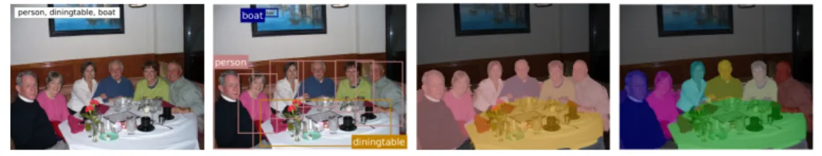
Given an image, information can be extracted on different levels. This is il-lustrated in Figure 1.1 where a few examples of image analysis tasks of different detail are shown. The focus of this thesis is semantic segmentation, which aims at understanding an image on a pixel level. This means that we want to assign a label to each pixel, describing the object it is depicting. For example, going back to Figure 1.1 we have assigned the label "person" to the pixels colored pink and the label "dining table" to the pixels colored yellow.

Semantic segmentation has numerous of applications. In robotics, agents are usually needed to extract useful information and understand their environment to perform tasks such as navigation and manipulation of objects. This is something that can be achieved with a camera and a semantic segmentation algorithm. Also, autonomous vehicles require a precise understanding of their surrounding to be able to make safe decisions in traffic. Semantic segmentation algorithms are also useful for numerous applications in medical research and clinical care, such as com-puter aided diagnosis and surgery assistance. Since many of the images handled in medical applications are three dimensional manual segmentation is time con-suming. Having an automatic method will in these cases save medical personnel a lot of time and be very helpful for time-critical tasks such as surgery planning.

Traditionally, semantic segmentation algorithms have been approached by ex-tracting some type of hand-crafted image features from the image. These features could be something as simple as color gradient or a more complex function of the

(18)

Figure 1.1: Example of scene understanding tasks with increasing detail from left to right. From left: image captioning, object detection, semantic segmentation and instance segmentation. This thesis focuses on semantic segmentation. Image modified from [1].

pixel values. A model relating these features to semantic classes is then created, or learnt from annotated examples, i.e. a set of images paired with their "true" semantic segmentations. During recent years most methods have moved from hand-crafted feature to using Convolutional Neural Networks (CNNs), capable of learning complex images features from data.

The introduction of CNNs for semantic segmentation meant a large improve-ment in performance and we are now able to create models that are fairly good at understanding the content of an image (given that it is similar to the images it has been trained on). A drawback with a CNN is however that they cannot explicitly take the dependencies between output variables, i.e. how the label of one pixel depends on the label of the output pixels, into account. This can however be done using Conditional Random Fields (CRFs), which have been used extensively for semantic segmentation. Because of this, many state-of-the-art methods combine a CNN and a CRF creating a Deep Structured Model (DSM) capable learning complex image features while still taking output dependencies into account.

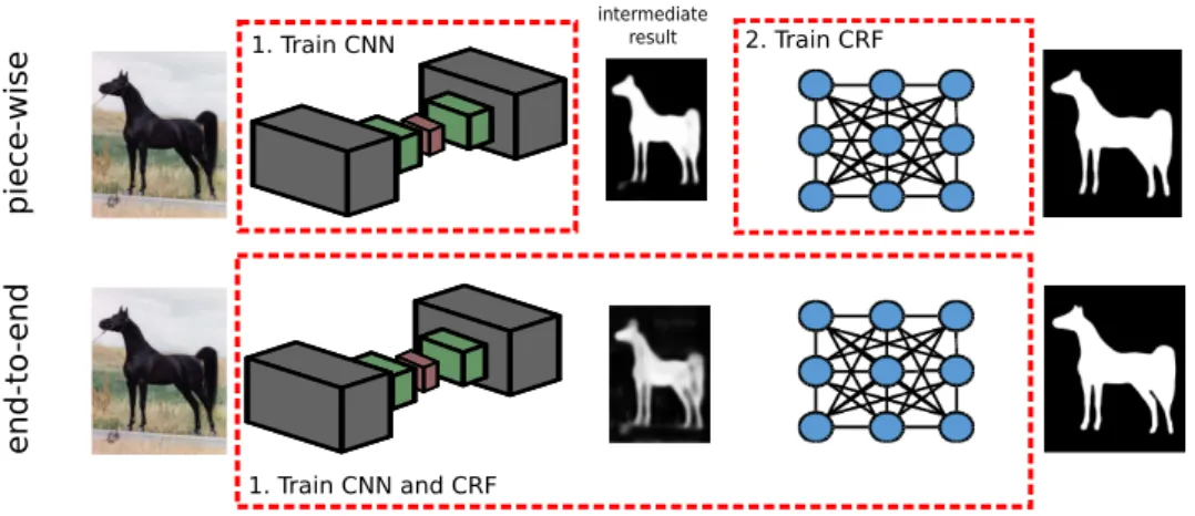
The parameters of these DSMs are usually learnt from data. This learning can be easily achieved by using traditional deep learning methods to train the CNN. Then, using the output of the CNN to form the CRF, learning the weight of the CRF. This approach, commonly referred to as piece-wise training, is suboptimal since the parameters of the CNN is learnt while ignoring output dependencies. A better approach is to train the CNN and CRF jointly, or end-to-end. This gives the CNN and the CRF a chance to learn how to interact to achieve better results, a sketch of piece-wise and end-to-end training of a DSM is shown in Figure 1.2.

(19)

1.1. Thesis Scope piece-wise end-to -end 1. Train CNN 2. Train CRF 1. Train CNN and CRF intermediate result

Figure 1.2: Comparison of piece-wise and end-to-end training of a deep structured model (DSM). For the piece-wise training (above) the CNN is trained first, as a second step the parameters of the CRF is trained keeping the weights of the CNN fixed. During end-to-end training (below) the weights of the CNN and CRF are jointly trained, giving them a chance to learn how to interact to achieve better results.

1.1 Thesis Scope

This thesis consists of three papers, all of them presenting solutions to semantic segmentation problems. The applications have varied widely and several different types of data have been considered, from 3D CT images to RGB images of horses to indoor scene understanding. The main focus has been on developing robust and accurate models to solve these problems. These models consist of a CNN capable of learning complex image features coupled with a CRF capable of learning dependencies between output variable, in our case pixel or voxel labels. Emphasis have been put on creating these type of models that also are possible to train end-to-end as well as the methods needed to enable this type of training.

1.2 Thesis Outline

The first part of this thesis consists of this introductory chapter, followed by Chap-ter 2 that provides some background knowledge needed to understand the papers included in this thesis as well as placing them in an academic context. Chapter 3 summarizes the work and contributions of this thesis as well as each paper sepa-rately. A brief discussion of future work is given in Chapter 4. Finally, the papers forming this thesis are appended in part II.

(20)

(21)

Chapter 2 Background

The focus of this thesis is to develop methods for semantic segmentation. Hence the background chapter will start off with a brief introduction to the problem of semantic segmentation. Afterwards a brief introduction to Convolutional Neural Networks (CNNs) as well as Conditional Random Fields (CRFs) will be given. Lastly, we will touch on the subject of end-to-end training of Deep Structured Models (DSMs), i.e. a combination of a CNN and a CRF. The sections in this chapter are by no means exhaustive but aim at giving the reader background knowledge enough to understand the included papers as well as place them in an academic context.

2.1 Semantic Segmentation

Semantic segmentation or scene labeling is the process of assigning each pixel of an image to the semantic class that it is depicting. The semantic class should depend on the surrounding information, or context, of the pixel. That means that we want to understand what the image is containing on a pixel level. What classes we are interested in dividing the image pixel in depends on the task and what information about our surrounding we are interested in. Given a set of images from a camera mounted on the front of a car we might want to classify each pixel as being one of ("driveable surface", "sidewalk", "pedestrian" etc.) while given a medical CT image of the abdomen we might want to classify pixels into different organs, or perhaps "tumour" and "not tumour". An example of visualizations of semantic segmentations is shown in Figure 2.1.

(22)

Figure 2.1: Two examples of semantic segmentations. To the left is an image from the Mapillary Vistas dataset [2], a street-level image dataset with 66 semantic classes. The semantic class of each pixel is visualized by overlaying the original pixel with the class color. To the right is a slice of a CT image from the MICCAI 2015 challenge “Multi-Atlas Labeling Beyond the Cranial Vault” [3] for organ seg-mentation in the abdomen. Here the voxels of a class are visualized by delineating them with the class color. Note that this is only one slice of the original 3D CT volume.

2.1.1 Evaluation

Given an image paired with a semantic segmentation it is quite easy for a human to visually evaluate the segmentation as good or bad. It is however important to quantify how good a segmentation is, both to be able to quickly evaluate a method applied to a big set of images and also to be able to compare between different methods. A straightforward metric to use is the pixel accuracy which is defined as the ratio between correctly classified pixels and total number of pixels. However, for some datasets, the per-pixel accuracy can be quite misleading. Given, for example, an image with a lot of pixels labeled as "background". A segmentation method simply assigning the "background" label to all pixels will get a high pixel accuracy even though it obviously performs poorly.

An alternative metric is the commonly used Intersection over Union (IoU) or "Jaccard" index. Given the set of pixels A segmented as a class and the set of pixels B belonging to the same class according to the annotation the IoU is

IoU= |A∩B|

|A∪B]. (2.1)

In terms of true/false positives/negatives we get

IoU= #tp

#tp+ #f n+ #f p, (2.2)

where#tpdenotes number of true positives,#f ndenotes number of false negatives and so on. The IoU can value between zero and one where a value of one means

(23)

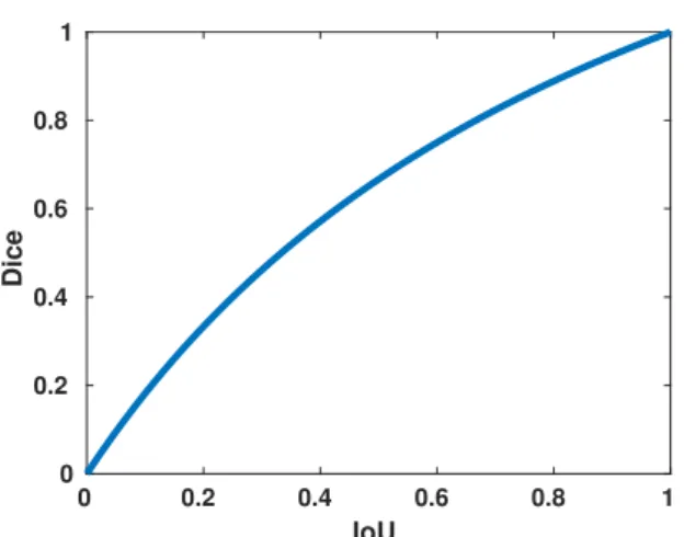
2.1. Semantic Segmentation 0 0.2 0.4 0.6 0.8 1 IoU 0 0.2 0.4 0.6 0.8 1 Dice

Figure 2.2: The Dice coefficient plotted as a function of the intersection over union. The Dice coefficient and intersection over union are two commonly used measure to quantify segmentation results.

a perfect overlap of the segmentation and the ground truth while a value of zero means no overlap at all. For multi-label problems the mean IoU (mIoU) over all classes is usually measured as an overall performance indicator of a segmentation method. A segmentation method simply assigning the "background" label to all pixels will get a quite low mIoU.

For medical image segmentation tasks the Sørensen-Dice coefficient, or sim-ply Dice coefficient, is a common metric. Using the previous notation the Dice coefficient is defined as

Dice= 2|A∩B|

|A|+|B|, (2.3)

which in terms of true/false positives/negatives can be written as Dice= 2#tp

2#tp+ #f n+ #f p. (2.4)

Similar to the IoU the Dice score can vary between zero and one. The relation between the Dice score and the IoU is Dice= 2 IoU/(1+IoU)which is visualized in Figure 2.2. As can be seen from the figure the Dice coefficient always corresponds to a lower intersection over union.

(24)

Deep Convolutional Neural Network

Input Image

Texton Feature

Extractor Boosting Classifier

Unary Result

Grid CRF

Input Image

Texton Feature

Extractor Boosting Classifier

Unary Result

Dense CRF

Input Image

Convolutional

Feature Extractor Linear Classifier

Unary Result

Dense CRF

Deep Convolutional Neural Network

Input Image

Convolutional

Feature Extractor Linear Classifier

Result CRF Inference Layer

Figure 2.3: Evolution of Semantic Segmentation systems. Initially, most ap-proaches relied on hand-crafted image features and a fairly simple CRF model, this is represented in the first row showing the "Textonboost" work [4]. The second row uses a more sophisticated CRF model, DenseCRF, presented in [5]. Later on, most works have replaced the hand-crafted features with features learned from data with a Convolutional Neural Network. An early example of this is [6]. Currently, several state-of-the-art method follows an approach that first appeared in [7] where the CRF inference is incorporated as a part of the neural network. Allowing learn-ing of the CNN and CRF weight simultaneously. This image is taken from [1] and result for this figure were obtained using the publicly available code of [6–10]

2.1.2 Development of Approaches

Semantic segmentation methods date back to the 1970s, e.g. [11, 12]. Many of the early approaches tried to divide the image into semantic areas and then relate these areas to each other using a fixed rule-based system. It was in most cases hard to get these kind of rule-based or grammar-based methods to generalize well and performance was quite poor for general images.

From the early 2000s up until now the popularity and performance of semantic segmentation methods has increased tremendously. The early methods utilized powerful tools such as image descriptor and machine learning [13]. The majority of these methods are data driven and require manually annotated images to be able to train the models. However, the models can of course be applied to unseen images and segment them into the semantic classes that were present in the man-ually annotated images. A lot of the state-of-the-art methods used a CRF to be

(25)

2.2. Learning Features

able to model interactions between the input images and output labels but also interactions between output labels. Given a CRF model most early approaches used the following pipeline

1. Extract features from the image. The features extracted could be the RGB color of the pixel and its surrounding pixel or some more advanced features such as Textons [14] or SIFT [4].

2. Use the extracted features and the annotated image to train an appearance model, i.e. a local classifier.

3. Use the output of the appearance model to form the unary term, i.e. the part of the CRF that models interactions between input and output.

4. Define, or learn from data, how the CRF should model interactions between output labels. Most commonly the type of interactions were pairwise, i.e. between the classes of two pixels.

5. Perform inference on the CRF model to segment an image.

This is of course a rough pipeline which a lot of methods will not fit into. In addition, a lot of extensions and variants exists for basically each step of the pipeline. Regarding, the first point of extracting features most work has moved from the carefully designed features to learning features from annotated data, usually with a CNN. This will be discussed thoroughly in Chapter 2.2. Also, several works have done data driven approaches to learn the pairwise interactions described by the CRF. In addition, several different types of CRF models have been proposed. A notable example is the DenseCrf presented in [5] where every pair of pixels is connected by a pairwise term in the CRF. Finally, during the last few years methods that learn the parameters of the CRF as well as the weights of the feature extracting CNN jointly have appeared. Two of them are the papers included in this thesis but a few more examples exist. Figure 2.3 provides a summary of this development.

2.2 Learning Features

As mentioned in Section 2.1.2 most methods for semantic segmentation nowadays use image features learnt from annotated data. The dominating approach is to use a CNN to learn these features and looking on most popular semantic segmentation benchmarks all top entries on the leaderboard use a CNN. In this section an introduction to Artificial Neural Networks (ANNs) and CNNs is given.

The idea behind ANNs and CNNs is not new. Already in the 1960s the bio-logically inspired Perceptron was introduced [15] which resembles the commonly

(26)

used ANNs of today. Also the idea of introducing spatial invariance in ANNs were presented already in 1980, when K Fukushima et al. introduced the "Neocogni-tron" [16]. During the 1980s and 1990s there were some progression in the field of neural networks but it wasn’t until a few years back that these types of methods got their breakthrough. In 2012 Krizhevsky et al. [17] presented "Alexnet", a CNN for classifying images of the ImageNet [18] dataset that achieved consider-ably better than the previous state-of-the-art. Since then, approaches using CNNs have become dominant in most detection and classification problems [19]. For the task of semantic segmentation a defining paper was J Longs et al. "Fully convo-lutional networks for semantic segmentation" [10] which introduced a method of transforming CNNs previously used for classification to efficiently segment an im-age. These types of "Fully Convolutional" networks are the standard for semantic segmentation nowadays.

2.2.1 Multilayer Neural Networks

The most common ANNs have a feed-forward neural network architecture. In these networks computations are done layer-wise, and the values of the data at one layer of the network depend only on computations in previous layers. In one layers of the network, the input to the layers is multiplied by a weight vectorWi

and a bias vector is addedbi according to

gi =Wihi−1+bi, (2.5)

here hi−1 is the output of the previous layer (or the input data if i is the first layer). The vectors hi are commonly referred to as hidden units (except for the

inputs h0 and the output hL) and their size depends on the size of the weight

matrices W. A weight matrix with less rows than columns will decrease the size of the hidden units vector. After this computation the outputgi is passed through

a non-linear activation function

hi =σ(gi). (2.6)

These computation layers are stacked on top of each other and the output of the last layer L is the output of the neural network y = hL. In modern literature,

(27)

2.2.2 Activation Functions

The activation functions are a crucial part of the neural network. If these were to be omitted the computations of the entire network would consist of only linear functions and could be replaced with an equivalent single matrix multiplication. In contrast, with non-linear activation function, it has been shown that a feed-forward neural network is a universal function approximator [20]. This means that, in theory, they can learn any function.

In the early days of neural networks, smooth non-linear activation functions were commonly used. Two examples of these are the Sigmoid, defined as

σ(x) = 1

1 +e−x, (2.7)

and the hyperbolicus tangen function σ(x) = tanhx. These functions are quite similar but differs in range, the output of a sigmoid lie within[0,1]while the output oftanh(x)lie within[−1,1]. The most popular activation function at the moment is the rectified linear unit (ReLU) [21] which is defined asσ(x) = max(0, x). Using ReLU activation functions in a neural network makes the training faster in general as well as allowing training of networks with more layers [19].

The activation function of the final layer is usually chosen differently to the intermediate activation functions. The choice usually depends on what task we are training the network to solve. For example, if we want to use the network to solve a regression problem we might not use any final activation function at all, allowing for unbounded output values of the network. If we instead are interested in image classification we could use a softmax activation function defined as

σ(x)j =

exj PN

k=1exk

for j = 1, ..., N. (2.8)

The softmax function outputs a set of values all between zero and one and which sum to one. The value of σ(x)j can hence be used as an estimation of the

proba-bility of the current input belonging to classj.

2.2.3 Convolutional Neural Networks

Convolutional Neural Networks [22] are designed to process data that has an in-herent grid-like structure, such as 2D RGB images, 3D videos or medical im-ages such as CT scans. Since many of these data types have a lot of input pa-rameters, an RGB image of standard size can for example be represented with

512×512×3 = 786432 values, the weight matrix W of a fully connected layer would become very large. This would make the computations very demanding while also giving the neural network an extremely large amount of weights, some-thing that might cause overfitting.

(28)

CNNs circumvent this problem by using a biologically inspired spatial weight sharing scheme [23]. Instead of learning full weight matrices for each layer a CNN learns a bank of filters for each convolutional layer. The intermediate values between layers are referred as feature maps and keep their spatial grid-like structure throughout the network. Learning filter, instead of full weight matrices, means that the same weight values will be applied at every spatial position for each layer, greatly reducing the number of weights needed to be learnt. This would be the equivalent of restricting the weight matrix of equation (2.5) to be a Toeplitz matrix. In addition, the convolutional layers are spatially invariant, meaning that input patterns found in different parts of an image will be processed similarly regardless of spatial position.

Another common component of a CNN are pooling layers. A pooling layer applies a rectangular window to each feature map forwarding for example the maximum number present in the window (for max-pooling layers). Pooling layers introduces an invariance to small shifts in input data while also reducing the spatial size of the feature maps, controlling the capacity of the neural network [19]. Adding pooling layers also enlarges the receptive field of higher level features. The receptive field of a feature is the part of the input image that might influence the value of the feature, a larger receptive field enables learning of more complex features. A common approach to building an CNN for image classification is to stack a couple of convolutional and pooling layers, adding activation functions (typically ReLU) after the convolutional layers. This enables the CNN to learn more complex and high-level features for each stacked layer. Ideally the first few layers learn to extract low level image features such as edges, lines and blobs while later layers extracts complex features such as faces, legs or wheels. Finally one or several fully connected layer can be applied to transform the features from spatially structured maps to for example a vector of estimated class probabilities.

Convolutional Layers

As mentioned the convolutional layers of a CNN learn a bank of filters. Given an input feature mapX of sizeWin×Hin×Fin, whereW is the width, H the height and F the number of feature maps. A trained bank of filters is applied according to

Yj =Bj + X

i

Wij ∗Xi, (2.9)

where Xi denotes the i-th feature map of X. The output feature map Y has a

size ofWout_×_Hout_×_Fout_{, padding can be used to keep the same width and height}

as the input feature map. The filter bank has a size ofK1×K2×Fin×Fout, where

K1 ×K2 is the size of each filter. For each output, optionally, a bias weight is learnt. Bj denotes this bias resized to the width and height of the output feature

(29)

map. The size of the filters differs from application to application but a size of

3×3 is most commonly used [24–26].

A variant of the convolutional layer designed to provide a greater increase of the receptive field, i.e. the region of the input that affects a particular unit of the network, between subsequent layers is theà-trous or dilated convolutions [27]. These convolutions uses a set of upsampled filters where only weights at everyl-th index is non-zero. Here, l is usually referred to as the dilation factor, note that dilated convolution withl = 1 is just standard convolution.

Pooling Layers

Pooling layers perform down-sampling of the image features [28]. Several types of pooling layers exist, the most common ones are max pooling and average pooling. These layers applies a fixed size window to the input feature map in strides. It then outputs the max (or average) of the values in this window. Choosing a stride equal to the window size results in non-overlapping regions that forwards information to the next feature map. Choosing a window size of 2×2 and a stride of 2 would result in a down-sampling of the spatial size of the feature map by a factor of 2.

2.2.4 Learning

Once the architecture of our CNN is set we can view it as a function approximator

f(x,θ), where x is the input and θ the learnable weights of each layer. This section will give a brief introduction to the most important parts needed for the learning process. Note that this is only applicable for supervised learning, where an annotated dataset is available.

Loss Function

A loss function is a way to quantify how well the CNN is performing, it hence measure the compatibility of the CNNs output, or prediction, to the ground truth label. The loss is generally defined for one sample of the dataset, and during learning the weights of the CNN, θ are adjusted to minimize the mean of the losses L(X,Y,θ) = 1 N X i Li(yi, f(xi,θ)). (2.10)

HereX,Y are the set of input and labels of a given dataset with N samples and

xi, yi denotes the data/label pair of one sample.

A commonly used loss function for classification tasks is the cross-entropy loss. For a CNN with a softmax activation function as a last layer, meaning that it outputs an estimation of the probabilities of inputxi belonging to each class, the

(30)

cross-entropy loss may be defined as

Li(yi, f(xi,θ)) =−log(fyi(xi,θ)). (2.11)

Here, fyi(xi,θ) is the estimate of the probability from the CNN that the input

belongs to the ground truth class yi. The name cross-entropy loss comes from

the fact that this loss minimizes the cross entropy between the distribution of the ground truth labels and the label distribution generated by the CNN, given that the samples are independent and identically distibuted random variables.

Loss Minimization

As previously mentioned the learning is achieved by minimizing a defined loss func-tion over the given dataset. Since there generally is not any closed-form solufunc-tion to the learning problem, θ∗ = arg max(L(X,Y,θ)), local optimization methods are often used. Most commonly a variant of gradient descent is used which updates the parameters of the CNN according to

θi+1 =θi−η∇θL(X,Y,θ), (2.12)

whereηis the step size or learning rate. For large datasets this is however inefficient and often a stochastic approximation of the gradient is used instead. This is called mini-batch gradient descent and is defined as

θi+1 =θi−η X

i∈B

∇θLi(yi, f(xi,θ)), (2.13)

where B is the batch which in turn is a subset of the complete dataset. Using a mini-batch of size one is referred to as stochastic gradient descent. There are several variants of this update rule, designed to reduce noise of the estimated gradient and accelerate convergence. Some examples are gradient descent with momentum [29], with Nesterov momentum [30], AdaGrad [31] and Adam [32]. All of these are first-order methods which means that they only require the calculation of the gradient with regards to the weights.

The gradient of the loss function with respect to all the weight of the net-work can be efficiently computed using the back-propagation algorithm [29]. The back-propagation algorithm is just a practical application of the chain rule for derivatives. Given the loss derivative ∂L_∂y with respect to the output of a simple layer described byy=f(x, θ), wherexis the input,ythe output andθthe weights. The loss derivative with respect to the input can calculated by simply applying the chain rule ∂L_∂x = ∂L_∂y∂f_∂x, similarly for the weight we get ∂L_∂θ = ∂L_∂y∂f_∂θ. Using this back-propagation we can start from the final layer of the network and calculate the loss with respect to the input of each layer, propagating the loss gradient all

(31)

through the network until we have calculated it with respect to every weight of the network.

Since the learning problem is non-convex and almost all methods are based on local optimization it is a possibility for the learning to get stuck in a poor local minimum. In practice, this is generally not a big problem, even for different initial conditions many networks reach a solution of very similar quality [19]. Recent work points towards the existence of a lot of saddle points in the loss surface that the learning algorithm might get stuck in [33, 34]. However, all of them have very similar and low values of the loss function and hence give a good enough solution.

Regularization

Overfitting is a term used for a model that performs well on the training data but poorly on unseen input data. Since a typical CNN contains a very large number of free parameters it is prone to overfitting. A large enough CNN could basically learn to "memorize" the training data instead of learning good rules that generalize to unseen data. Because of this, several regularization methods meant to prevent the CNN to overfit have been developed.

Ideally, we would like to just add training data until the CNN is incapable of overfitting. Annotating new data is however a timely process which we generally want to avoid. An alternative to adding new training data is to perform data aug-mentation on the already available data. This means changing the samples of the data in an slightly randomized way during training. Common augmentation op-erations used for image tasks are, random cropping of the image, random rotation or simply adding noise to the pixel values.

Another fairly simple regularization technique is weight decay. This means adding an extra term to the loss function that penalize large values of the parame-ters of the CNN. For the case ofL2 _{weight decay the term}_λ1

2

P

iθ2i, whereλis the

weight decay strength, is added to the loss function in (2.10). ForL1_{regularization} we instead add the termλP

i|θi|, favoring sparse solutions.

Two additional, very popular, regularization techniques are Dropout [35] and Batch Normalization [36]. These are added as separate layers to the CNN and have different functionalities during learning and during inference. Dropout works by only keeping the values of each neuron non-zero with set probability p, the others are set to zero. During inference, all neuron values are kept but scaled with a factor p. Batch Normalization shift the values of the features to have zero mean and unit variance for each mini-batch during training. In addition to avoid overfitting to some extent this also allows the use of a higher learning rate during training [36].

(32)

CNNs for Semantic Segmentation

The task of annotating data is considerably harder and more time-consuming for semantic segmentation where each pixel need to be annotated compared to image classification where only one label per image is needed. This restricts the size of available datasets for semantic segmentation and there are no available datasets of the same size as for example Imagenet [37]. Due to this, many popular CNNs for semantic segmentation have a classification counterpart that has been trained on the million images of Imagenet. The architecture of the classification CNN is changed to enable dense output maps, transforming it to a segmentation CNN. However, the weights of the first few layers are kept with the motivation that these layers have learnt to extract meaningful image features during the extensive classification training. This approach have shown to be preferable to training from scratch for many segmentation tasks, even for images fairly different from the Imagenet data [38–40].

Repurposing a classification network for semantic segmentation is not entirely straight-forward. As previously mentioned a defining paper for ths was "Fully convolutional networks for semantic segmentation" by J Longet al. [10] where they presented segmentation version of several classification network that were state-of-the-art on Imagenet at that time. The fully connected layers of these networks were transformed to convolutional layers with filter size1×1, which changes the previous classification scores to spatial feature maps. These feature maps, together with feature maps earlier in the CNN were upsampled using deconvolution layers [41] and merged providing dense output predictions for images of arbitrary size. These CNNs can then be trained for segmentation end-to-end using a pixel-wise version of the cross-entropy loss presented in Section 2.2.4.

Despite the success of fully convolutional networks of [10] this architecture has several drawbacks. Pooling layers are great for image classification, enabling the CNN to learn complex high-level image feature. It is however not ideal since per-forming pooling operations means loosing spatial information of where the image features came from in the image. Some works have tried to get rid of the pooling layers entirely [42] and other types of layers has been introduced in an effort to keep spatial information while still achieving large receptive field. An example of this is the dilated convolutions mentioned in Section 2.2.3 [27].

Many recent works considering CNNs for semantic segmentation try to design networks that are able to learn high-level image features while not losing spatial information. Some examples include encoder-decoder networks such as Segnet [43] and U-Net [44] as well as PSP-Net [45] that processes features on different resolution in separate paths.

(33)

2.3. Learning Structure

2.3 Learning Structure

As mentioned in Section 2.2.3 CNNs are good at modeling complex relations be-tween input data and output data. They cannot however explicitly take dependen-cies between output variables into account. In addition, they are often trained with a pixel-wise loss function, disregarding the fact that the output data is actually structured.

A way of taking output structure into account which also allows for explicit modeling of dependencies between output variables is using Probabilistic Graph-ical Models (PGMs). A PGM models a probability distribution over a set of random variables whose structure is defined via a graph. In this thesis we will focus on Conditional Random Fields (CRFs) that are commonly used for semantic segmentation.

2.3.1 Conditional Random Fields

Conditonal Random Fields (CRFs) models the conditional probability, P(Y|X)

of an output set Y = {Y1, ..., YN} given and input X. Working with images, X

denotes the image values and we generally associate one input and one output variable with each pixel. For semantic segmentation each output Yi is assigned

a value from a finite set of possible states L = {l1, l2, ..., lL}, where each state

represent a class label. The dependencies between output variables are described by an undirected graph whose vertices are the random variables{Y1, ..., YN}. The

conditional probability for the CRF can be written as

P(Y =y|X) = 1

Z(X)exp(−E(y,X;w)), (2.14)

where E(y,X;w) denotes the Gibbs energy function with respect to the assign-ment of labels to the output variables y ∈ LN_{. The parameters,} _w_{, of the CRF}

can either be hand-crafted from prior knowledge or learnt from data. Z(X)is the partition function given by

Z(X) = X

y∈LN

exp(−E(y,X;w)). (2.15) It is hence a normalization constant making the conditional probabilities sum to one. Note that the sum is over all possible combination of label assignments available, it is hence computationally costly to evaluate the value of the partition function.

For most image applications the Gibbs energy function decomposes over unary and pairwise terms,i.e. terms depending on only one and two variable respectively.

(34)

The energy can be written as E(y,X;w) = X u∈V ψu(yu,X;w) + X (u,v)∈E ψuv(yu, yv,X;w), (2.16)

note that the graph structure defines what terms are present in this energy. For

ψuv(yu, yv,X;w) to be non-zero node u and v must share an edge. The terms

ψu(yu)and ψuv(yu, yv,X;w)are commonly referred as unary and pairwise

poten-tials respectively.

Potential Types

The unary potentials, also known as the data cost, of the CRF energy are often obtained from a pixelwise classifier estimating the class probabilities of each pixel. Commonly the term for each pixel is set to

ψu(yu =lp) =−w1log(P(yu =lp|X)), (2.17)

whereP(yu =lp|X)is an estimate of the probability of pixel u belonging to class

lp.

For the pairwise potential,as a first step, the connectivity or structure of our graph needs to be defined. This specifies what pairwise terms should be included in the energy, and also which output variables should depend on each other. A simple and commonly used structure is the nearest neighbour connectivity where pixels are connected through an edge to its neighbours only. The size of the neighbourhood might vary but for 2D images a size of four or eight is common. An example of this structure can be seen in Figure 2.4.

The pairwise potentials,ψuv(yu =lp, yv =lq, I;w), defines the cost of assigning

label lp to pixel u and label lq to pixel v . It can hence be used to enforce

con-sistency and structure in the output. As an example, for semantic segmentation, we generally want neighbouring pixels to have the same labels. A type of pairwise term that enforces this is the Potts model given by

ψuv(yu =lp, yv =lq, I;w) =w21lp6=lq, (2.18)

where 1lp6=lq denotes the indicator function equaling one if lp 6= lq and zero

oth-erwise. This pairwise term can be generalized in several ways, for example we might want to weight the cost of assigning different labels to neighbouring pixel differently depending on if they have similar color or not. This can be achieved by adding a weighting term according to

ψuv(yu =lp, yv =lq, I;w) =w21lp6=lqe

−(xu−xv)2_, _(2.19)

wherexu and xv are the pixel values of pixelu andv. This type of pairwise terms

(35)

2.3. Learning Structure y₁ x₁ y₅ x₅ y₉ x₉ y₁₃ x₁₃ y₂ x₂ y₆ x₆ y₁₀ x₁₀ y₁₄ x₁₄ y₃ x₃ y₇ x₇ y₁₁ x₁₁ y₁₅ x₁₅ y₄ x₄ y₈ x₈ y₁₂ x₁₂ y₁₆ x₁₆

unary

pairwise

Figure 2.4: CRF with a simple nearest neighbour connectivity, neighbourhood size

four. The variables yu are assigned class labels while the variables xu represents

the pixel values.

Both of these pairwise terms are constructed using prior knowledge, such that neighbouring pixel often have the same label unless there is a change in contrast. This is of course not true in all cases and several works have instead tried to learn the pairwise term from data [46, 47]. In Paper I we present a CRF model with more general pairwise potentials that can be learnt from data.

Using a neighbourhood only consisting of neighbouring pixels limits the extent on how far across the image information can propagate. A natural way to increase this limit is to increase the size of the neighbourhood, for example connecting all pixels closer than d pixels apart. The extreme of this would be to connect all pairs of pixels which is done for the denseCrf model. The denseCrf model were popularized by [5], that presented a method to perform efficient inference for these types of CRFs. The pairwise terms for dense CRFs also include a weighting on the distance between two pixels, hence the strength of the pairwise term decays exponentially with the distance between the pixels.

It is also possible to include potentials that depend on more than two pixel labels, i.e. higher order potentials. Higher order potential can for example be used to enforce consistency within superpixels or utilize object detection results for semantic segmentation [48–51].

(36)

Inference

Given an imageX the inference problem, giving a semantic segmentation, equates to finding the maximum a posteriori labeling of the model in equation 2.14. Finding the minimizer to the Gibbs energy, i.e.

y∗ = arg min

y

E(y,X;w), (2.20)

is an equivalent problem. This problem is in general NP-hard [52], typical ap-proaches to solving it can hence be divided into two categories, exact algorithms that only applies to special cases of the energy and approximate solutions. We will provide a few examples here but for an extensive overview of approaches we refer to [53, 54].

If we deal with a binary segmentation problem, i.e. only are interested in two classes, and if the energy is submodular the globally optimal solution can be found using the graph cuts method [54]. This approach can be extended to multi-label problems using theα-expansion [55], however we lose the guarantee of finding the global optimum.

Several popular methods are based on a relaxation of the original problem, these are usually the most efficient ones for performing inference in denser CRFs. One example is the mean-field method where the original distribution isP(y|I)is approximated with a fully factorized oneQ(y). The optimization is then done by minimizing the Kullback–Leibler divergence between the two distributions. Other approaches rely on a continuous relaxation of the Gibbs energy, and then using local search methods to find a local minimum of the energy. This type of methods have been shown to outperform mean-field on several tasks [56] and is the approach used in Paper I.

Parameter Learning

The learning problem consists of estimating the parameters of the CRF,w, based on a training set(Y(k)_,_X(k)₎N

k=1. The goal with the training is that if inference is performed for an input image from the data set, we want a solution close to the ground truth labeling. An intuitive approach to the learning problem is based on the maximum likelihood principle. This means finding the set of parameters that maximizes the probability of the training set.

A major difficulty when performing maximum likelihood training for CRFs is that it requires computation of the partition function for each training instance and for each iteration of a numerical optimization algorithm. This is of course computationally expensive and makes learning infeasible for CRF models used for semantic segmentation. Most popular learning methods hence makes approx-imations that simplifies the computation of the partition function. Mean field is

(37)

2.4. End-to-End Learning

an example of this where the fully factorized distribution simplifies computation of the partition function [5]. Piece-wise training is also an option which only re-quires computation of local normalization factor over fewer variables [57,58]. Other methods instead try to estimate the partition function using sampling [59].

Another approach is to use a learning method that avoids the computation of the partition function, for example learning a model that maximizes the margin between the energy of the ground truth and any other output configuration [60,61]. This can be formulated as

max

w ζ

s.t. E(Y,X(k);w)−E(Y(k),X(k);w)≥ζ ∀k and Y 6=Y(k).

(2.21) Since, there is an exponential amount of constraint in this optimization problem it is not feasible to solve it as is. A solution to this is to iteratively add the constraints that currently is furthest away from being satisfied [62]. This learning method is utilized in Paper II.

2.4 End-to-End Learning

Combining CNNs and CRFs is a powerful approach for dense classification tasks such as semantic segmentation. The CNNs ability to learn complex high-level im-age features paired with the CRFs ability to model output dependencies generally yields impressive results. However, many existing approaches use a two step train-ing process to learn the weights of the CNN and CRF. Firstly, the CNN is trained to perform pixel-wise segmentation on the available data set. Secondly, the CRF is trained keeping the unary potentials fixed (although based on the output of the CNN). This is often referred to as piece-wise training and is non-ideal since the CNN is learnt while ignoring dependencies between output variables.

Instead, a better solution would be to perform end-to-end training. This means jointly training the CNN and the CRF at the same time. In this way the CNN and the CRF get the chance to learn how to interact and exploit complementary information to achieve as good of a result as possible. During recent years several examples of these deep structured model trained end-to-end have been proposed in the literature [7, 47, 63–65]. This section gives a very brief introduction to some of these methods, for more details we refer to the recently published tutorial paper on the subject [1].

(38)

2.4.1 CRF Inference as a Neural Network Layer

Given a CRF inference method only consisting of differentiable operations, these operations can be implemented as neural network layers. By implementing the back-propagation routines for this layer, which amounts to applying the chain rule for derivative, the error derivatives with respect to the parameters of the CRF can be computed during training. In addition, the error derivative with respect to the output of the CNN can be computed and the error can be propagated all the way back through the CNN. This enables the parameters of both the CRF and the CNN to be updated simultaneously using for example stochastic gradient descent. This was shown to be possible for the mean-field inference algorithm [7]. In Paper I we show that this is possible for gradient-based CRF inference as well.

2.4.2 Back-propagating CRF Learning Objective

Many of the approaches for CRF parameter learning presented in Section 2.3.1 can be abstracted to minimizing a global objective L. This global objective depends on the samples of the data set, the parameters of the CRF as well as the output of the CNN, denotedz, used to create the CRF potentials. If we are able to calculate the gradient of this global objective with respect to the CNN output,∇zL, we can

back-propagate this gradient back through the CNN to calculate ∇θL, where θ

are the weights of the CNN. The weights can then be updated using local search methods. Examples of methods in this category are [47, 59, 63]. In Paper II we present a method for doing this utilizing the max margin training approach for CRFs introduced in Section 2.3.1.

(39)

Chapter 3 Summary

The focus of this thesis is to develop DSMs for semantic segmentation. Emphasis have been put on creating models that are possible to train end-to-end as well as the methods needed for training. Paper I and Paper II are obvious examples of this. In Paper III a robust segmentation method for abdominal organs using CNNs is developed. The original idea was to use the DSM and training routines developed in paper II and add it to this framework as well. However, this did not actually improve the results much and was hence discarded. This brings up an important question, what types of CRFs are needed to improve on the results of a CNN? This is something that will be discussed in Chapter 4.

Regardless of using a DSM or not Paper III presents a robust method for abdominal organ segmentation. The paper combines a robust organ localization with the use of specialized organ CNNs for segmentation. Since segmentation is a key problem in medical image analysis, a method for organ segmentation can be crucial for numerous applications in medical research and clinical care such as computer aided diagnosis and surgery assistance. In addition, robustness is something that is generally highly valuable for medical applications. At the time of writing this thesis the development of deep learning methods for 3D medical application is a popular research subject and many large scale research projects exist on this topic [66].

Paper II introduces a method of training a DSM end-to-end using a max-margin objective. However, several restrictions to the CRF is needed to be able to do the training efficiently. The CRF used has a pairwise term where each pixel is only connected to its closest neighbours. This can easily be extended, however the method uses graph-cut inference of the CRF during training which becomes slow for densely connected CRFs.

In Paper I a framework for training DSMs with more expressive CRFs is pre-sented, here a newly developed approximate inference method of the CRF is used. However, we would like to point out that this should not be seen as a strictly better approach than the one used in Paper II. The max-margin approach of Paper II

(40)

has the advantage of using a fast and exact inference algorithm of the CRF. In addition the learning approach used have been shown to generalize well, even for smaller datasets. Something that suited the experiments on smaller medical data sets presented in the paper well.

The more expressive DSM presented in Paper I is however suitable for larger datasets with more semantic classes. This enabled us to do experiments on for example the PASCAL VOC 2012 segmentation benchmark [67] consisting of several thousands of annotated images and 21 semantic classes.

At the moment segmentation is all about the evaluation numbers. The meth-ods achieving the highest mean Intersection over Union on the major benchmarks get the most attention. This is of course positive in the manner of encouraging researchers to develop practically useful and accurate methods. The major bench-marks are also an invaluable tool for comparing different methods. However, the chase for better numbers combined with the use of very data-hungry deep learning brings on a research pipeline that usually is 10% method development and 90%

parameter tuning and learning hacks. Something that also makes reproducing previous work harder.

Unfortunately, the methods presented in Paper II and Paper I fail to achieve state-of-the-art results on the major benchmarks. We have however successfully shown the usefulness of both approaches in each paper respectively. Perhaps most notable for Paper II is the performance of the method on smaller medical datasets. For Paper I the model has the ability to improve on very strong CNN baseline trained on a lot of additional data, even though the DSM were only trained end-to-end on a subset of the data.

The remainder of this chapter will contain short summaries of the papers in-cluded in this thesis. In addition, the thesis author’s contribution to each paper will be stated.

(41)

3.1. Paper I

3.1 Paper I

M. Larsson, A. Arnab, F. Kahl, S. Zheng, and P. Torr. ”Revisiting Deep Structured Models in Semantic Segmentation with Gradient-Based Inference”. Submitted to SIAM Journal on Imaging Sciences.

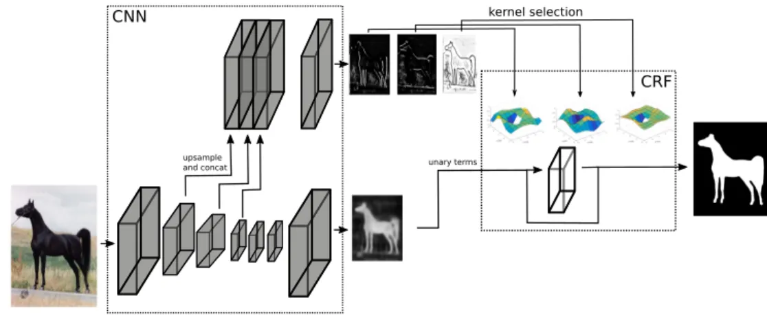
In this paper we move from binary label CRFs with short spatial pairwise interactions to CRFs being able to handle multiple labels and learn pairwise inter-actions on larger distances. We present an inference technique based on gradient descent on the Gibbs energy of the CRF. This inference method consists only of differentiable operations which enables us to unroll the CRF inference as a number of update steps of a Recurrent Neural Network (RNN). During learning, we can also back-propagate through the RNN and do end-to-end training of the entire model.

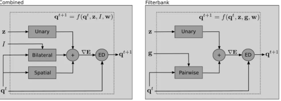
Two different types of CRF models are presented in the paper. The first one consists of a spatial pairwise term as well as a high-dimensional bilateral kernels. In contrast to many previous works we don’t restrict these two kernels to have Gaussian shape but allow for arbitrary shape of the spatial and bilateral kernels. In addition, we introduce a new type of potential function which is image-dependent like the bilateral kernel, but an order of magnitude faster to compute since only spatial convolutions are employed. The major contributions of the paper are

• A new model for a pairwise CRF potential which is image-dependent like the bilateral kernel, but does not require high-dimensional filtering. It is based on a learned 2D filter bank which makes both inference and learning an order of magnitude faster than high-dimensional filtering approaches.

• A new optimization method for CRF inference based on gradient descent that enables end-to-end training.

• We show that our inference method supports learning pairwise kernels of ar-bitrary shape. The learned kernels are empirically analyzed and it is demon-strated that in many cases non-Gaussian potentials are preferred.

Author contribution. I did the method development and implementation with support from F. Kahl. Experiments were run by me, A. Arnab and S. Zheng. The writing was done by me and A. Arnab while the initial idea was proposed by F. Kahl.

(42)

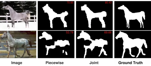
70.85 80.43

Image

53.79

Piecewise

69.66

Joint Ground Truth

Figure 3.1: Comparison of piecewise versus joint training of a deep structured model for some hand-picked example. The number shown in the upper right corner is the Jaccard index (%).

3.2 Paper II

M. Larsson, J. Alvén and F. Kahl. ”Max-Margin Learning of Deep Structured Models for Semantic Segmentation”. Scandinavian Conference on Image Analysis

(SCIA),28–40, 2017.

This paper presents a method for learning the parameters of a Deep Structured Model which in this case refers to a CNN paired with a CRF. The learning problem is formulated as a Structured Support Vector Machine (SSVM) and we show that it is possible to calculate the derivative of the objective with respect to the output of the CNN. This enables us to back-propagate all through the layers of the CNN and learn the weights of the CNN and the CRF at the same time. Since the SSVM uses a max-margin loss function that generally gives good generalization capabilities of the trained model this method is especially suitable for application where labelled data is limited.

Figure 3.1 shows a comparison of the piecewise and jointly trained models. As can be seen the model where the CNN and CRF have been trained jointly performs for better, avoiding error such as cutting of the legs of the horse. This is because the CNN has learnt to compensate for the slight shrinking effect of the CRF.

Author contribution. I did the method development and implementation with support from F. Kahl. The writing was done by me and J. Alvén while the initial idea was proposed by F. Kahl.

(43)

3.3. Paper III Merging ROI Localization Spleen CNN Aorta CNN . . . Organwise voxel classiﬁcation

Figure 3.2: Graphical representation of the method presented in Paper I.

3.3 Paper III

M. Larsson, Y. Zhang and F. Kahl ”Robust Abdominal Organ Segmentation Using Regional Convolutional Neural Networks”. Submitted to Applied Soft Computing.

This paper presents a method for segmenting 13 different abdominal organs utilizing CNNs. The method can be divided into two main steps. Firstly, an efficient and robust feature registration method is applied estimating the center-point of each organ. Secondly, a convolutional neural network performing voxelwise classification is applied to a region, defined by a prediction mask placed at the estimated organ center-point. The prediction mask is created using the ground truths of each organ in the training set. The approach of first localizing a region of interest for each organ transforms the problem the CNN has to solve from a large multi-label problem to 13 smaller binary-labels problems. We can hence train smaller CNNs and more specialized, or regional, networks that only need to differentiate between a certain organ and the background.

During the development of this method and at the writing of the first draft of this paper there were very few examples of deep learning methods applied to medical 3D segmentation tasks and none for this specific tasks. Since then, there has been a lot of development in this area and several papers have been published further showing that deep learning methods can perform really well on these types of tasks.

Author contribution. I did the method development and implementation with support from Y. Zhang and F. Kahl. The writing was done by me while all authors contributed to the main idea.

(44)

(45)

Chapter 4 Outlook

The field of semantic segmentation has moved at a high pace during the last few years, especially when it comes to methods based on CNNs. Every month there is a new CNN with a different architecture pushing state-of-the-art further. During 2015 and 2016 the results of CNNs presented for semantic segmentation could be greatly increased by adding a CRF [7, 26]. This is mainly due to the fact that the architectures of the networks used during this time did not allow the CNN to learn interactions over long ranges. In addition the downsampling of the pooling layers resulted in a loss of spatial information that prohibited the accurate segmentation of fine edges between classes, hence the output usually became "blobby". Both of these errors are something that the most commonly used CRF models excel at. However, during late 2016 and 2017 several new CNNs have been proposed, raising state-of-the-art, that do not use a CRF for post-processing [45, 68]. This indicates that the type of CRFs commonly used in semantic segmentation might not be necessary for these large scale problems with a lot of annotated data.

An additional detail with the CRFs is that inference for most of the commonly used models are still fairly slow, especially for the powerful dense models with edge-aware pairwise potentials. Some work has been done on creating alternatives to these CRFs that are less computationally demanding but still has the ability to refine segmentations near edges [69, 70]. This is also adressed as part of Paper I.

So, for CRFs and DSMs to be really useful for these large scale segmentation problem in the future there are two improvements needed. Firstly, the inference needs to be faster, adding a CRF should not speed down the inference or training considerably. Unless, of course the gain in performance is worth it. Secondly, there might be a need to rethink the type of models we are using and try to create CRFs that are better suited to correct the errors that the new state-of-the-art CNNs do. Moving away from the large scale segmentation benchmarks there are still a lot of applications where adding a CRF gives a big increase in performance. Looking at datasets with slightly smaller training set, DSMs tend to perform better in general. CRFs are also a good way to include prior knowledge in you segmentation pipeline.

(46)

Previous work has shown that geometric constraints, such as convex or star shaped for-ground objects only can be enforced by a CRF [71, 72].

4.1 Future Work

4.1.1 Output Structure

At the moment many of the top entries of the major segmentation benchmarks train CNNs with a pixel-wise loss function, disregarding the fact that the output is structured. Modern CNNs have the capability to, and probably do, implicitly learn that there is structure in the output. However, actually taking the output structure into account, whether by using a CRF or in some other way, could be beneficial. There is hence interest in continuing the work on end-to-end training of DSMs, both trying to improve computation speed and to design more expressive models. In addition it would be interesting to do more work on DSMs for medical image segmentation where more application-specific types of CRFs might be needed.

Another interesting approach to taking output structure into account was in-troduced in [73], which used a Generative Adversarial Network (GAN) for semantic segmentation. The idea was that the discriminator would be able to learn how an ground truth segmentation should look like. Hence during training, the generator, that also performs the actual segmentation, would have to output realistic seg-mentation to trick the discriminator. In this way the output of the segseg-mentation CNN would have to follow, and hence learn, the output structure of the segmenta-tions. This introduces an interesting opportunity to learn output structure without having to perform CRF inference.

4.1.2 Weak Supervision

Annotating data for semantic segmentation is a tedious task, especially for 3D med-ical images. There has hence been an increase in approaches that utilize weakly annotated data, for example image tags or bounding boxes of objects [74–77]. Hav-ing powerful weak supervision learnHav-ing methods would mean less needed annotated data for application specific segmentation tasks, which would be crucial for many situations. An interesting idea of utilizing GANs for this task was presented last year [78], something that might be interesting to build upon.

One of our current projects is addressing the task of semantic localization, i.e. utilizing semantic cues to estimate the pose of a camera given the image taken and an 3D map. One step of the pipeline requires accurate semantic segmentations for road-scenarios. What we noticed, when trying some state-of-the-art models trained on the cityscapes dataset [79], was that these performed very poorly on our images. This despite the fact that the environments were fairly similar. We

(47)

4.1. Future Work

are now working on improving segmentation results on these images by utilizing a dataset consisting of a large 3D map. Using this we can extract correspondences where we have two images of the same place, we can hence train the CNN to be consistent for the part of the images that show the same object or objects. The hope is that this would give us a CNN that generalizes better to new conditions, without having to manually annotate new images.

(48)

End-to-End Learning of Deep Structured Models for Semantic Segmentation