White Rose Research Online
[email protected]
Universities of Leeds, Sheffield and York
http://eprints.whiterose.ac.uk/
This is a copy of the final published version of a paper published via gold open access
in
Frontiers in Computational Neuroscience
.
This open access article is distributed under the terms of the Creative Commons
Attribution Licence (
http://creativecommons.org/licenses/by/3.0
), which permits
unrestricted use, distribution, and reproduction in any medium, provided the
original work is properly cited.
White Rose Research Online URL for this paper:
http://eprints.whiterose.ac.uk/83946
Published paper
Finding minimal action sequences with a simple evaluation
of actions
Ashvin Shah * and Kevin N. Gurney
Department of Psychology, The University of Sheffield, Sheffield, UK
Edited by:
David Hansel, University of Paris, France
Reviewed by:
Benoît Girard, Centre National de la Recherche Scientifique and Université Pierre et Marie Curie, France
Gianluigi Mongillo, Paris Descartes University, France
*Correspondence: Ashvin Shah, Department of Psychology, The University of Sheffield, Western Bank, Sheffield S10 2TP, UK
e-mail: [email protected]
Animals are able to discover the minimal number of actions that achieves an outcome (the minimal action sequence). In most accounts of this, actions are associated with a measure of behavior that is higher for actions that lead to the outcome with a shorter action sequence, and learning mechanisms find the actions associated with the highest measure. In this sense, previous accounts focus on more than the simple binary signal of “was the outcome achieved?”; they focus on “how well was the outcome achieved?” However, such mechanisms may not govern all types of behavioral development. In particular, in the process of action discovery (Redgrave and Gurney, 2006), actions are reinforced if they simply lead to a salient outcome because biological reinforcement signals occur too quickly to evaluate the consequences of an action beyond an indication of the outcome’s occurrence. Thus, action discovery mechanisms focus on the simple evaluation of “was the outcome achieved?” and not “how well was the outcome achieved?” Notwithstanding this impoverishment of information, can the process of action discovery find the minimal action sequence? We address this question by implementing computational mechanisms, referred to in this paper as no-cost learning rules, in which each action that leads to the outcome is associated with the same measure of behavior. No-cost rules focus on “was the outcome achieved?” and are consistent with action discovery. No-cost rules discover the minimal action sequence in simulated tasks and execute it for a substantial amount of time. Extensive training, however, results in extraneous actions, suggesting that a separate process (which has been proposed in action discovery) must attenuate learning if no-cost rules participate in behavioral development. We describe how no-cost rules develop behavior, what happens when attenuation is disrupted, and relate the new mechanisms to wider computational and biological context.
Keywords: action discovery, reinforcement learning, intrinsic motivation, optimal control, redundancy, dopamine
1. INTRODUCTION
Animals are capable of executing a huge variety of move-ments and behaviors, to which we refer collectively as actions. Importantly, animals are able to discover the actions, including sequences of actions, that affect the environment and prefer-entially recruit them in order to explore the environment and accomplish tasks. This process is often studied using the proto-cols of operant conditioning (Thorndike, 1911; Skinner, 1938), in which the animal, free to execute many actions, receives a bio-logically rewarding outcome if it executes a particular action or sequence of actions. For example, in Edward Thorndike’s clas-sic experiments (Thorndike, 1911), a hungry cat was placed in a “puzzle box” and could escape to get food only after it had exe-cuted one or several actions, such as pressing a lever and pulling a string. When first placed in the box, the cat would execute many actions, most of which did not affect the box’s door, until it hap-pened to press the lever and then pull on the string, after which the box’s door opened. With repeated trials, the cat executed fewer of the irrelevant actions, and executed only the actions that led to the door opening.
As with many tasks, Thorndike’s puzzle box has massive redundancy in that the outcome can be achieved in many ways (such as by executing irrelevant actions as well as the actions that open the door). Animals resolve this redundancy to a large extent—they are able to achieve the outcome without executing more actions than necessary. We refer to such behavior as the minimal number of actions that achieves an outcome, or, sim-ply, theminimal action sequence. Animals are able to discover the minimal action sequence through their own interactions with the environment rather than just from external instruction. How this behavior is learned has been (and is still) the focus of much research in psychology and neuroscience (e.g.,Staddon and Cerutti, 2003; Pearce, 2008; Balleine et al., 2009) and, because it describes how learning agents learn from their own experiences, artificial intelligence, and robotics (e.g.,Sutton and Barto, 1998; Hart, 2009; Konidaris, 2011).
achievement of the outcome itself is one obvious signal that can be used to determine if a particular action sequence has achieved the outcome. In addition, in most previous accounts, actions are further evaluated in that actions are associated with a measure of behavior that is higher for actions that lead to achieving the outcome with a smaller total number of actions, and learning mechanisms adjust the tendencies to select actions so as to max-imize that measure of behavior. Thus, shorter action sequences that achieve the outcome are preferred because they are deter-mined to be “better” than longer action sequences that achieve the outcome, and the minimal action sequence is the “best” or “opti-mal” with respect to that measure of behavior. In other words, most previous accounts are concerned not with just the simple evaluation of “was the outcome achieved?”; rather, they are con-cerned with “how well was the outcome achieved?” where “how well” is in reference to the measure of behavior the learning rule maximizes.
A commonly used computational framework with which to study animal learning processes is a class of optimal control meth-ods called computational reinforcement learning (RL) (Bertsekas and Tsitsiklis, 1996; Sutton and Barto, 1998). RL is inspired in part by animal learning (particularly Thorndike’sLaw of Effect, Chapter 5 ofThorndike, 1911), and neuroscience research in the 1990s (Ljungberg et al., 1992; Schultz et al., 1993) and subsequent research reveal RL’s ability to describe biological learning pro-cesses (Houk et al., 1995; Schultz et al., 1997) (see alsoShah, 2012
orNiv, 2009for reviews relating RL with psychology and neuro-science). In RL, a learning agent discovers behavioral policies that maximize a measure of behavior that is a function of numerical signals—usually referred to as “reward signals”—delivered by the environment. Typically, a positive numerical signal is delivered when the learning agent achieves the outcome of interest (sim-ulating the biologically rewarding outcome the animal receives when it accomplishes an operant conditioning task), addressing the question “was the outcome achieved?” In addition, the ques-tion “how well was the outcome achieved?” is usually addressed by incorporating one or both of the two following types ofcost. The first type of cost is that every executed action incurs anexplicit action costin the form of a negative numerical signal (represent-ing quantities we presume the animal encodes internally that it seeks to minimize, such as muscular effortPedotti et al., 1978; Fagg et al., 2002; Todorov and Jordan, 2002; Shah et al., 2004). If each executed action incurs a similar explicit cost, the mini-mal action sequence incurs the fewest negative numerical signals. The second type of cost is that the magnitudes of the numerical signals—in particular, the magnitude of the positive numerical signal delivered when the outcome is achieved—decreases with temporal delay. Thistemporal discount has often been studied in experimental psychology and behavioral economics by pre-senting an animal with a choice of two actions: one leads to a rewarding outcome after a short delay, the other after a long delay (Samuelson, 1937; Chung, 1965; Logan, 1965; Green and Myerson, 2004). If the two actions lead to an outcome of the same magnitude of reward (such as the same amount of food), the ani-mal is more likely to choose the action associated with the short delay. The temporal delay is thought to add animplicit cost by
decreasing the perceived magnitude of the reward. If each exe-cuted action takes a similar non-zero amount of time to execute, the positive numerical signal upon achieving the outcome is tem-porally discounted the least with the minimal action sequence.
A learning agent using RL rules modifies its behavior through its own interaction with the environment (executing actions and observing the consequences).Model-freeordirectRL methods use experience exclusively, while other types of RL methods also use models of the environment to behave or modify behavior (Sutton and Barto, 1998; Daw et al., 2005). We focus on model-free meth-ods in this paper. The RL rule generates reinforcement signals based on an error in prediction of the measure of behavior. If an action’s consequences result in a higher measure of behavior than expected, reinforcement signals that compare the experienced measure with the expected measure increase the tendency to select that action (the action isreinforced), and decrease the tendency if the consequences result in a lower measure than expected. When that measure of behavior is expressed as described in the previous paragraph, an action that leads to achievement of the outcome with a shorter action sequence is considered to be “better” than other actions that also achieve the outcome and the tendency to execute it is greater than the tendency to execute other actions (it is preferred). Thus, RL rules using that measure of behavior focus on “how well was the outcome achieved?”
While mechanisms that use such measures of behavior may account for many types of behaviors, such as acting to maximize rewards received, they may not apply to all types. In particular, Redgrave et al. (Redgrave and Gurney, 2006; Redgrave et al., 2008, 2011, 2013; Stafford et al., 2012; Gurney et al., 2013) discuss how the unexpected occurrence of a salient outcome causes the animal to repeat preceding actions, even if the outcome is not biologically rewarding (see alsoHorvitz, 2000; Barto et al., 2004). With con-tinued repetition, the animal discovers the actions that achieve the outcome and represents them as a single action in a process referred to asaction discovery. Importantly, however, the process of action discovery is thought to be driven by the unexpected occurrence of the outcome. As described in detail inRedgrave and Gurney (2006), biological reinforcement signals in action discov-ery occur too quickly to evaluate behavior beyond an indication of the outcome’s occurrence—learning mechanisms in action discovery may be driven by a prediction error regarding the out-come’s occurrence, but not an error in prediction of a measure of behavior that is higher for actions that lead to achievement of the outcome with a shorter action sequence. In other words, action discovery is thought to be driven by mechanisms that focus on the simple binary signal of “was the outcome achieved?” and not by the continuous signal of “how well was the outcome achieved?” (Action discovery is considered to be part of broader class of
If action discovery does not focus on “how well was the outcome achieved?” how can the minimal action sequence be discovered in action discovery? Here, we describe a computa-tional mechanism by which this can occur. We implementno-cost
learning rules, based on canonical RL rules (Sutton and Barto, 1998), that do not use either of the two types of cost described above. If the outcome is achieved, no-cost learning rules gener-ate reinforcement signals that increase the tendency to execute every action that was executed en route to the outcome, but at a rate that decreases with temporal distance from the outcome. Importantly, in no-cost rules, actions that lead to achievement of the outcome are each associated with the same measure of behavior (indicating that the outcome was achieved) as opposed to a measure of behavior that is higher for actions that lead to achievement of the outcome with a smaller number of actions. No-cost rules focus on the simple evaluation of “was the outcome achieved?” as opposed to “how well was the outcome achieved?” They represent a possible computational mechanism by which the minimal action sequence can be developed that relies on different types of information and processes than previous accounts and is consistent with the process of action discovery.
Recent modeling work (Chersi et al., 2013) has shown that learning rules similar to the no-cost rules we describe in this paper can be used to discover the minimal action sequence. However, they use networks of spiking neurons to investigate neural mech-anisms of goal-directed and habitual control and do not directly address the questions we raise in this paper. From the presented results, it is not clear if the learning rule can reliably discover the minimal action sequence if there is massive redundancy, i.e., if a very large number of action sequences of varying lengths can achieve the outcome.
Here, we simulate artificial agents using no-cost learning rules acting within discrete-state discrete-action environments in tasks in which there is massive redundancy and the outcome depends on sequences of more than a few actions. Discrete-state discrete-action environments and tasks are commonly used to describe and evaluate RL algorithms (Sutton and Barto, 1998). The no-cost rules we implement are able to discover and execute, for a tempo-rary yet substantial amount of time, the minimal action sequence. This behavior can be described as optimal with respect to a mea-sure of behavior that is influenced by explicit action costs and/or temporal discounting of numerical signals, but it emerged “for free” without taking these types of cost into account. We go on to describe how such behavior arises from no-cost rules.
Behavior under no-cost rules consists of the minimal action sequence for a substantial period of time; however, if actions con-tinue to be reinforced according to no-cost rules for an extended amount of time, extraneous actions are developed—because any action that leads to achievement of the outcome is associated with the same measure of behavior in no-cost rules, behavior does not converge with extended training. Thus, stable behavior with no-cost rules requires that reinforcement signals be attenuated with a separate process as learning progresses with a separate pro-cess. Interestingly, the reinforcement signals, mediated by phasic dopamine neuron activity (Wickens et al., 2003) in biological operant learning, also appear to undergo attenuation (Ljungberg et al., 1992; Schultz et al., 1993, 1997) and a similar process has
been proposed in action discovery (Redgrave and Gurney, 2006; Redgrave et al., 2008, 2011, 2013). According to action discov-ery, reinforcement signals, mediated by phasic dopamine neuron activity, are attenuated by a separate process that is contingent on the ability to predict the occurrence of the outcome. In the work presented here, we do not seek to model the separate pre-diction process underlying reinforcement attenuation but, rather, we examine resulting behavior if the attenuation were disrupted (e.g., due to disorders in prediction or reinforcement functions). We discuss the significance of this process and no-cost learning rules in relation to other theories of reinforcement attenuation, namely, descriptions of phasic dopamine neuron activity in terms of an error in prediction of a measure of behavior that is different for different actions (Houk et al., 1995; Schultz et al., 1997), in the Discussion section. Elements of this work have been presented in poster format (Shah and Gurney, 2011).
2. METHODS
2.1. ENVIRONMENT
We subject learning agents to tasks in state discrete-action environments (Figure 1) in which a “state” is an abstract representation of the current situation or context from which to take an action, and an “action” causes a transition from one state to another. The environment is Markov: the effect of an action depends only on the current state and not on previous states vis-ited. Such environments can be represented in different ways. A typical representation used to demonstrate and evaluate RL algo-rithms is thegrid-worldenvironment (Figure 1top row) (Sutton and Barto, 1998), in which states are visually represented in a spatial grid, states that can be reached from each other with one action are placed next to each other, and the effects of an action are analogous to movements in the grid-world. Thus, states that can be reached from each other with a small number of actions are placed closer together than states that require a larger number of actions to be reached from each other. By using such a represen-tation, a behavioral trajectory that follows “the minimal action sequence” from one state to another is readily apparent as the shortest trajectory when visually illustrated. Although the grid-world representation suggests a maze to test navigational abilities, it is misleading to think of it in this way. It merely provides a visu-ally accessible representation of an abstract sequential decision task. Using Thorndike’s puzzle box as an example, suppose that the cat scratched itself, pulled the chain, pawed at the door, bat-ted the wall, licked its paw, and then pressed the lever to open the door. This sequence of actions would be represented as a longer trajectory than if the cat only pulled the chain and pressed the lever to open the door.
FIGURE 1 | Illustrations of the environments we use.Each “state” is represented as a small square or rectangle within the environment. Actions can be executed that transition the agent from one state to another (see text). In all environments, the state colored blue (labeledss) is the starting
state and the state colored red (so) is the goal state and represents
achievement of the outcome. In the grid-world (top left), states labeleds1
ands2are referred to in the text. In the grid-world with obstacles, transitions
into obstacle states (highlighted in green and with a “×”) are prevented. In both grid-worlds, four cardinal and four diagonal actions are available from
each state; actions are deterministic. In warped-world 1 (bottom left), only four cardinal actions are available. Because states are not aligned vertically, actions to the north or south stochastically transport the agent into one of the two states that overlap the current state, weighted by the relative amounts the states overlap the current state (see Supplementary Material for details). In warped-world 2, four cardinal and four diagonal actions are available, but actions between “big” and “small” states are different than actions between big and big states and actions between small and small states (see Supplementary Material for details).
reached or when a maximum number of time steps has elapsed (a “time-out”). As discussed inSutton and Barto (1987), this explicit segregation is a simplification as animal learning processes may not incorporate mechanisms that are dependent on the concept of an episode or trial. An effect similar to an explicit segrega-tion can be accomplished by providing an explicit indicasegrega-tion at the start of a trial (as is often the case in experimental tasks)
or by imposing a lengthy delay between trials (as, for example,
Izhikevich, 2007 does in simulation), but the explicit segrega-tion of the episodic task framework is mathematically simpler (Sutton and Barto, 1998) for our purposes. Episodic tasks are commonly used in RL models of human and animal tasks (e.g.,
in general (e.g., Sutton and Barto, 1998; Konidaris and Barto, 2009).
In the basic grid-world task (Figure 1 top left), states are arranged in a 12×12 grid. At the beginning of each trial, the current time step,t, is set to 1 and the agent is placed in a fixed starting state,ss, highlighted in blue inFigure 1. At each time step, the agent chooses an action,a, from the set of possible actions: four cardinal and four diagonal actions in the grid-world. Action effects are deterministic, and actions that would cause a transition off the grid result in no change in state. The trial terminates if the agent transitions into stateso(highlighted in red), which signifies the achievement of the outcome, or after 115 time steps in the grid-world environments. This somewhat arbitrary “time-out,” about 10%× number of states× number of possible actions, allows for massive redundancy in that there is a very large num-ber of action sequences of varying lengths that can reachsofromss
within the time-out. (In contrast, if the time-out were the same as the minimal number of actions that could achieve the outcome, the task would be non-redundant: only behavior that uses the minimal number of actions to achieve the outcome could achieve the outcome within the time-out).Trefers to the last time step of a trial and is always≥the minimal number of actions it takes to achieve the outcome and≤the time-out. In addition, a numerical signal,rt, is delivered at each time step (this signal is different in
with-cost vs. no-cost measures of behavior, as described below). Thegrid-world with obstacles(Figure 1top right) is the same as the grid-world except that transition into obstacle states (green squares with a “×”) is prevented. The obstacles prevent a spatially direct trajectory fromss toso. In the grid-world without
obsta-cles, short-length trajectories are easily reached from each other, so the chances of getting stuck in a local minimum are not high. We use the grid-world with obstacles to examine behavior in envi-ronments in which some short-length trajectories (i.e., above and below the obstacles) are not easily reached from each other, in which case the chances of getting stuck in a local minimum have increased.
While these tasks are not strictly navigation tasks, they can serve as abstract representations of tasks with some underly-ing geometric structure. To examine how behavior developed under different learning rules may be interpreted in such cases, we examine behavior in two spatially “warped” environments as well. Inwarped-world 1 (Figure 1bottom left), the number of states along the horizontal dimension is larger at higher verti-cal locations than that at lower vertiverti-cal locations. Thus, states do not represent the underlying spatial geometry uniformly, e.g., states at higher vertical locations represent a smaller spatial area than states at lower vertical locations. Also, only the four cardinal actions are available. Because the states are not aligned verti-cally, the effects of actions north and south in warped-world 1 are stochastic (see Figure caption and Supplementary Material for details). Inwarped-world 2(Figure 1bottom right), “small” states, which are in the middle and lower areas of the environ-ment, represent smaller spatial areas than do “big” states, which are in the outer areas of the environment. Cardinal and diagonal actions are available; actions between small and big states have slightly different effects than do actions from big to big states or actions from small to small states (see Supplementary Material for
details). The time-outs for warped-worlds 1 and 2 are 276 and 286 steps, respectively.
We use the warped-worlds to examine possible ways by which spatially indirect behavior can be accounted if overall behavior was observed but the underlying representations of states and actions were not known. One possible account of spatially indi-rect behavior is that the state representation is spatially uniform (as in grid-worlds), the animal assigns a higher cost to particu-lar actions made a particuparticu-lar locations, and behavior is developed with a learning rule that incorporates explicit action costs. For example, a behavioral trajectory that travels east and then north may be taken as evidence that trajectories that travel north and then east are more costly, or that horizontal actions executed at higher vertical locations are more costly than horizontal actions executed at lower vertical locations. Similarly, trajectories that avoid the center of an environment may be taken as evidence that trajectories that go through the middle of the environment incur greater action costs.
We suggest that spatially indirect behavior can also be accounted for with mechanisms that do not incorporate explicit action costs. Instead, such behavior may emerge from nonuni-form representations of the environment already in place through prior experience and developmental processes. Spatial represen-tation and cognition is a topic of much current research (Moser et al., 2008; Chen et al., 2014; Willis et al., 2014) and nonuniform representations occur in many central nervous system struc-tures involved with different modalities (van Essen et al., 1984; Curcio et al., 1990; Kurtzer et al., 2006; Graziano and Aflalo, 2007; Scott, 2008; Lillicrap and Scott, 2013). We use the warped-worlds to examine behavior resulting from mechanisms that do not incorporate explicit action costs if the state representation is nonuniform in the spatial domain.
2.2. WITH-COSTvs.NO-COSTMEASURES OF BEHAVIOR
A measure of behavior, often referred to as the return in RL (Sutton and Barto, 1998), is determined byrt, the numerical
sig-nal delivered at each time step. The return at timet of a trial is the sum of these signals fromt+1 to the end of trial:Rt =
T
i=t+1ri, whereTindicates the last time step of a trial. (Recall
thatt=1 at the beginning of a trial and, because a trial termi-nates whensois achieved,Tdepends on the number of actions
taken during the trial, andTwill always be less than or equal to the time-out). We differentiatewith-costandno-costmeasures of behavior by the information communicated byrt.
2.2.1. With-cost measures
Underwith-costmeasures of behavior,rtis used to associate
dif-ferent actions with difdif-ferent measures of behavior if they lead to achievement of the outcome with different numbers of actions.
rt is an explicit action-dependent negative numerical signal (a
“cost”) of−1 if a cardinal action was selected at timetand−√2 if a diagonal action was selected (e.g.,Sutton and Barto, 1998; Shah and Barto, 2009). Transition intoso delivers a positive numer-ical signal of ro= +20 instead of the action-dependent cost.
BecauseRt is the sum of action-dependent costs (androifsois
achieved),Rt can take on a range of values:Rt is different for
the action sequence fromsstosothat is associated with the high-est return follows the spatially direct trajectory (dashed line in
Figure 1), which is also the minimal action sequence. Longer action sequences are associated with a lower return because more negative signals contribute to the return. In this way, the with-cost measure of behavior is often different for different actions selected from a particular state or different action sequences and can be used in learning rules that focus on “how well was the outcome achieved?”
We note that the return can also be expressed as Rt =
T
i=t+1γi−t−1ri (Sutton and Barto, 1998), where γ captures
the effect of temporal discounting: if 0≤γ <1, then numer-ical signals delivered with a long delay (t + delay) will have less weight onRt than signals delivered with a short delay. For
example, ifrt =ro= +20 if the outcome is achieved butrt =0
otherwise, andγ <1, then the return will be less if the outcome is achieved after a larger number of actions than if the out-come is achieved after a smaller number of actions. As described in the Introduction, temporal discounting can also be thought of as a type of cost. Because explicit action costs and tempo-ral discounting have similar effects on the return—longer action sequences that achieve the outcome are associated with a lower measure of behavior than shorter action sequences that achieve the outcome—we include only explicit action costs in this paper for simplicity, i.e., ifγ were included in the equations,γwould be set to 1.
2.2.2. No-cost measures
Under no-cost measures of behavior, rt=0 at every time step
except ifso is reached, at which point r
t =ro= +20 (and, as
above, there is no temporal discounting ofrt). Thus, under
no-cost measures of behavior,Rtcan take on only two values (0 or
ro= +20) and is the same for everytduring the trial: 0 ifsowas
not achieved during the trial, andro= +20 if so was achieved
during the trial. In this way, the no-cost measure of behavior is the same for any action sequence that achieves the outcome and can be used in learning rules that focus on “was the outcome achieved?”
2.3. ACTION SELECTION
The tendency to select actionawhen in statesis represented by
Q(s,a). Actions are selected stochastically according to their rela-tive tendencies (via a “softmax” function, as described inSutton and Barto, 1998):
p(s,a)= e
Q(s,a)/τ
A
i=1eQ(s,ai)/τ
, (1)
wherep(s,a) is the probability of selecting actionafrom states
andτ (=1.5) controls the stochasticity. InitialQ(s,a) are set to zero. Learning rules described below modifyQ(s,a) for each vis-ited state and action based on experience. If the tendency to select an action is increased (ifQ(s,a) increases), that action is said to bereinforced.
2.4. MONTE CARLO AND TEMPORAL DIFFERENCE LEARNING RULES
We implement several learning rules expressed in the form of one of two types of RL rules (Sutton and Barto, 1998) that modify
Q(s,a) based on experience. The first type, called Monte Carlo (MC) rules, useRt directly to deliver reinforcement signals only
at the end of the trial. The state visited at timetis denotedstand
the action executed from that state is denotedat.Q(st,at) for each
visited (st,at) is modified at the end of a trial with the actualRt
experienced during the trial:
Q(st,at)←Q(st,at)+αλT−t−1[Rt−Q(st,at)], (2)
whereα (=0.1) is a step-size andλ(0≤λ≤1) defines an eli-gibility trace (Pavlov, 1927; Sutton and Barto, 1981, 1998; Klopf, 1982; Wörgötter and Porr, 2005). The eligibility trace allows for
Q(st,at) fortbeforeT(the last time step of the trial) to be
modi-fied and controls the rate at which it is modimodi-fied. If 0< λ <1, the eligibility trace is decaying in time andQ(st,at) for each (st,at)
is modified with a rate that is lower fortfar fromT, i.e.,Q(st,at)
fortearly in a trial is modified at a lower rate thanQ(st,at) for
tlater in a trial. Ifλ=1, the eligibility trace is non-decaying and
Q(st,at) for each (st,at) is modified at the same rate. We refer to
these rules as MC(λ).
The second type of learning rule is a temporal difference (TD) rule (Sutton, 1988; Sutton and Barto, 1998), in which
Q(st−1,at−1) is modified at every time step withrtandQ(st,at):
Q(st−1,at−1)←Q(st−1,at−1)+α[rt+Q(st,at) −Q(st−1,at−1)] (3)
(this particular formulation is the “SARSA” learning rule,
Rummery and Niranjan, 1994). EachQ(st−1,at−1) is modified
to be closer tort+Q(st,at) (and thus indirectly toRt). (Note
that there is no temporal discount term). This rule does not have an eligibility trace. However, it can be considered a special case of similar rules that do have eligibility traces (Sutton and Barto, 1998), but withλ=0. We thus refer to it as TD(0).
2.5. WITH-COST vs. NO-COST LEARNING RULES
Q(s,a) for each (s,a) visited during a trial are modified by learn-ing rules toward the measure of behavior to be expected if action
awere execute from states.
2.5.1. With-cost learning rules
For comparison purposes, we implement two standard RL algo-rithms (Sutton and Barto, 1998) using the with-cost measure of behavior: MC(1) (whereλ=1) and TD(0), referred to here as
with-cost rules.
When modified according to with-cost rules,Q(st,at) for each
Q(st,at) visited during a trial is modified toward the return (Rt)
according to the with-cost measure of behavior. The with-cost measure of behavior includes the sum of explicit action costs received during the trial after selecting actionatfrom statestand,
if the outcome is achieved during the trial,ro= +20. (Q(s,a) is
modified toward the actual experienced return in MC rules, and the nextrtandQ(s,a) in TD rules).Rtcan thus take on a range of
described in the Introduction and earlier in the Methods, tempo-rally discountingrtwould also have this effect). Because they use
with-cost measures of behavior, with-cost learning rules focus on “how well was the outcome achieved?”
2.5.2. No-cost learning rules
We suggest that a simple rule using a no-cost measure of behav-ior (which is not influenced by explicit action costs) would be an MC rule because the reinforcement signal is generated at only one time step (T) and only one return need be generated. We also suggest that it use a decaying eligibility trace. We thus imple-ment an MC rule with a no-cost measure andλ=0.7, referred to as ncMC(0.7) (where “nc” indicates “no-cost”). We implement two otherno-cost rulesfor comparison purposes: ncMC(1) (with
λ=1) and ncTD(0).
When modified according to no-cost rules, Q(s,a) is not modified toward a return that incorporates explicit action costs. Instead, the return can take on one of only two values under no-cost measures (0 ifsois not achieved orr
o= +20 ifsois achieved),
and eachQ(s,a) during a trial is modified toward the same value. No-cost rules use no-cost measures of behavior and focus on “was the outcome achieved?”
BecauseQ(s,a) for each state and action approach the same value under no-cost rules in our simulations, and actions are selected stochastically according to Q(s,a), behavior according toQ(s,a) modified with no-cost rules does not converge with extended experience. Rather,Q(s,a) will approachrofor all states
and actions in our simulations and, eventually, each action will be chosen with equal probability. In order for behavior under no-cost rules to stabilize, another process must attenuate reinforce-ment signals. We do not model this process here so as to describe the behavioral patterns that would result from inappropriate con-tinued reinforcement. (Also, note that in our simulations, there is no state or action from which it is not possible to achieveso. In tasks and environments in which there do exist states and actions from which it is not possible to achieveso,Q(s,a) for those states and actions will remain at 0).
2.6. EXPERIMENTS
Arun consists of an agent undergoing 200,000 trials. (A large number of trials was chosen so as to better expose the effects of reinforcement for an extended period of time under the differ-ent rules). Twdiffer-enty runs for each learning rule were conducted using the grid-world environment. Behavior was examined attest points(every 100 trials for the first 1000 trials; every 1000 trials after that), during whichα=0 and fivesample trialsusing theQ -values from the test point were run. Thus, 100 sample trials (five sample trials for each of the twenty runs) for each test point were used to report behavior.
In addition, twenty runs using ncMC(0.7) were conducted for the grid-world with obstacles and the two warped-worlds.
3. RESULTS
3.1. DISCOVERY OF THE MINIMAL ACTION SEQUENCE IN THE GRID-WORLD
We use the word “behavior” to refer to the agent traversing a series of states by executing a sequence of actions. For the
grid-world (Figure 1top left), behavior that follows the spatially direct trajectory (dashed line) is the minimal action sequence because it achieves the outcome—reachessofromss—using the minimal
number of actions. If an outsider observed this behavior, and was not aware of the mechanisms by which it was developed, he may describe it as optimal with respect to a measure of behavior that is higher for actions that lead to achieving the outcome with a smaller total number of actions, such as a measure of behav-ior in which every executed action is accompanied by an explicit cost (negative numerical signal) (as described in the Methods).
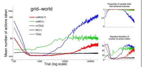
Figure 2left shows the mean (across all sample trials) number of actions at each test point for each learning rule. Note that standard deviation (Figure 2bottom right) is very low at sample trials for which the mean number of actions is very low.Figure 2
top right shows the proportion of sample trials that achieved the outcome at each test point for each learning rule.
As seen inFigure 2and consistent with descriptions inSutton and Barto (1998), the two standard with-cost rules, MC(1) and TD(0), develop the minimal action sequence in that behavior converges to a low number actions (stochasticity inherent in action selection prevents any rule from executing only the min-imal action sequence). This is unsurprising because they incor-porate the with-cost measure of behavior in which each action incurs an explicit cost.
[image:8.595.305.551.513.630.2]Behavior under no-cost rule ncMC(1) reliably achieves so, but ncMC(1) was not able to discover and execute (on aver-age) behavior that uses a low number of actions. No-cost rule ncMC(0.7) was able to discover and execute, for trials 400 to 11,000, the minimal action sequence. Similarly, no-cost rule ncTD(0) was able to discover and execute, for trials 400–2000, the minimal action sequence. Although the minimal action sequence can be described as optimal with respect to the with-cost mea-sure of behavior in that it reliably executes actions associated with the highest with-cost measure of behavior (the minimal action sequence), it is important to note that ncMC(0.7) and ncTD(0) use the no-cost measure of behavior, in which any action sequence that achieves the outcome is associated with the same measure
FIGURE 2 | Left:mean (across all sample trials) number of actions at each test point for each learning rule (see legend for color scheme). Trial time-out is indicated by “max” (115) on the vertical axis. The minimum number of actions needed to achieveso(8) is indicated by “min.” Note that the
horizontal axis uses a log scale.Bottom right:standard deviation of the number of actions at each test point for each learning rule.Top right:
of behavior. We explain how no-cost rules discover the minimal action sequence in the next subsection.
Behavior under with-cost rules converges with continued rein-forcement for an extensive period of time. Behavior under no-cost rules does not; rather, the mean number of actions increases with continued reinforcement for an extensive period of time (up to 200,000 trials in our simulations).
3.2. HOW NO-COST RULES DISCOVER THE MINIMAL ACTION SEQUENCE
The ability of ncMC(0.7) to discover the minimal action sequence can be understood by examining how the decaying eligibility trace (λ <1, see Methods) affects the rate at whichQ(s,a) for each action executed at each state visited en route to the out-come is modified. Letst be the state visited at timet, andat be
the action executed from statest. Recall that, under ncMC(0.7),
Q(st,at) for each visited (st,at) is modified toward the same value
at each trial:ro= +20 ifsowas achieved, 0 if not. (In contrast,
in with-cost rules, which use the with-cost measure of behavior,
Q(st,at) for each visited (st,at) is modified toward different
val-ues because they lead to action sequences of different lengths.) However, becauseλ <1, the rate at whichQ(st,at) is modified by
ncMC(0.7) depends on the temporal distance oftfromT(where
Tindicates the time step at the end of the trial):Q(st,at) fort
early in a trial (and thus far fromT) are modified at a lower rate thanQ(st,at) fort late in a trial. This has the effect of
reinforc-ing actions that lead to shorter action sequences that achieve the outcome at a greater rate than actions that lead to longer action sequences that achieve the outcome, even though allQ(st,at) are
modified toward the same value.
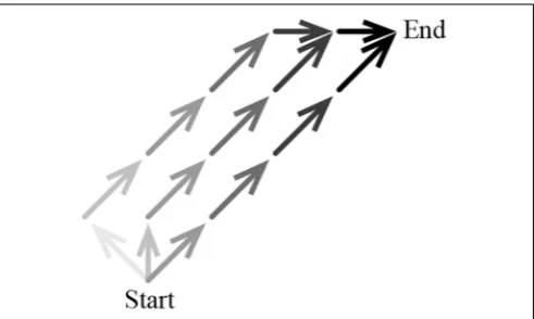
[image:9.595.46.292.513.660.2]This idea is illustrated in Figure 3, which is a simplified schematic of three sequences of actions from one state (“Start”) to another (“End”). The darker the arrow representing the action, the greater the rate at which that action is reinforced if the out-come is achieved: actions executed at a closer temporal distance to End are reinforced at a greater rate than actions executed at a further temporal distance to End. As in the grid-world, the min-imal action sequence consists of taking the action northeast to
FIGURE 3 | Simplified schematic of three sequences of actions from “Start” to “End.”Each action is represented by an arrow; the darker the arrow, the greater the rate at which the tendency to select the action is modified.
move directly from Start to End (right-most action sequence in
Figure 3). A slightly longer action sequence involves taking action north from Start and then moving directly to End (middle action sequence). The longest of the three action sequences involves tak-ing action northwest from Start and then movtak-ing directly to End (left-most action sequence). Because taking action north from Start leads to a longer action sequence than taking northeast from Start, action north from Start is reinforced at a lower rate than action northeast from Start. Similarly, action northwest from Start is reinforced at an even lower rate.
Under ncMC(0.7), all actions that were executed during tri-als in which the outcome was achieved are reinforced toward the same measure of behavior (ro= +20), but those that lead
to shorter action sequences are reinforced at a greater rate than those that lead to longer action sequences. In other words, the minimal action sequence is reinforced at a greater rate than all other sequences that achieve the outcome. Also, because action selection—behavior—is based on a softmax function of
Q(s,a) (see Methods), actions associated with a higher Q(the minimal action sequence) are more likely to be executed for a period of time. Thus, ncMC(0.7) discovers and executes, for the vast majority of the first 11,000 trials, the minimal action sequence. (As described later, because each Q(st,at) is
mod-ified toward ro= +20 if the outcome is achieved, eventually
all action sequences will be equally likely to be executed— extraneous actions will be selected with continued reinforcement and extensive experience).
Similar reasoning explains how ncTD(0) discovers the min-imal action sequence: because information at time t (rt and
Q(st,at) for the TD rules in this paper) are used to modify
Q(st−1,at−1) in the TD rules we use (Sutton, 1988; Rummery and Niranjan, 1994; Sutton and Barto, 1998), information avail-able attlate in a trial must propagate over several trials to (st,at)
visited attearlier in a trial. Thus,Q(st,at) fortlater in a trial are
modified at a greater rate than that fortearlier in a trial under ncTD(0) as well. (This feature also offers an explanation for the observation that behavior as developed by with-cost rule TD(0) actually uses fewer actions (on average) from trials 400 to 2000 than at later trials,Figure 2).
As demonstrated with behavior developed under rule ncMC(1), simply reinforcing behavior that achieves so, and
decreasing the tendency to select behavior that does not achieve
so within the time-out, provides a small bias toward—but not reaching—the minimal action sequence. ncMC(0.7) and ncTD(0) reinforce all actions that achievesoas well, but, because the rate of reinforcement is greater for actions executed in closer temporal proximity toT, ncMC(0.7) and ncTD(0) can discover and execute the minimal action sequence for a temporary but substantial period of time.
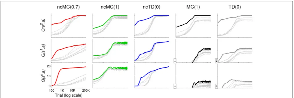
These concepts are also illustrated inFigure 4, which graphs, for each learning rule, the meanQ(s,a) for each action at states
ss, s1, and s2 (highlighted inFigure 1top left) as a function of trial number. State s2 is spatially close toso (the outcome); ss
(the starting state) is spatially far fromso; ands1is in between.
Q(s,a) for the most direct action (northeast for each of the three states) is highlighted in color (according to the legend in
FIGURE 4 | Mean (across the 20 runs) Q(s,a) at each test point for states ss, s1, and s2 (highlighted in Figure 1) for learning agents in
the grid-world using the different learning rules.The learning rules are indicated at the top. Q(s,a) for a= northeast, which is the action that leads to the shortest action sequence in each case, is drawn with a thick line in color according to the legend in Figure 1. That of all other actions are drawn with thin gray lines. The horizontal axis (log
scale) is the same in each graph, as is the vertical axis. The downward arrow at the bottom of the vertical axis in the graphs in the lower right indicates that Q(s,a) in these graphs actually fall below the lower limit of the vertical axis (i.e., they are negative) during early trials. However, we cut off these graphs to enable a visually clearer comparison of
Q(s,a) evolution in the latter stages of training under the different learning rules.
more likely to be executed attcloser toTthan those from states farther fromso. Thus, if the outcome is achieved, actions from
s2 are reinforced at a greater rate than those from s1, which are reinforced at a greater rate than those from ss (Figure 4).
Also, in all no-cost rules, at statesss, s1, and s2, action north-east is reinforced at a greater rate than other actions (this effect is much stronger for rules ncTD(0.7) and ncTD(0) than for ncMC(1)).
The use of stochastic action selection allows all (s,a) to even-tually be visited many times. As a result,Q(s,a) for each (s,a) gets modified towardro= +20 ifsowas achieved (0 if not) under
no-cost rules. Thus, eventually allQ(s,a) will be close to+20 with continued reinforcement (trials during whichsois not achieved prevent them from reaching+20). Because actions are selected stochastically based on Q(s,a), with extensive experience and continued reinforcement, all actions will eventually be equally likely to be selected and behavior as developed by no-cost rules will deviate from the minimal action sequence. This can be seen inFigure 4, left three columns. In contrast, because Q(s,a) as developed by with-cost rules converge to different values, depend-ing on the number of actions executed subsequently, behavior as developed by with-cost rules stabilizes to close to the mini-mal action sequence even with continued reinforcement (Figure 4
right two columns).
3.3. PATTERN OF DEVELOPMENT OF EXTRANEOUS ACTIONS
Under ncMC(0.7), Q(s,a) increases toward ro= +20 (if so is
reached) at a greater rate for (s,a) visited closerT(the last time step of a trial) than for (s,a) visited further fromT(Figures 3,
4). Thus, if reinforcement under ncMC(0.7) continues for an extended amount of time, extraneous actions will be selected at states closer toso(which is a termination condition for a trial) ear-lier in experience than at states closer toss.Figures 5,6illustrate this pattern.
Figure 5shows, for sample trials that achievedsoin the grid-world, the mean shortest distance from the line segment between
ss and so of the first four visited states (after ss) of the trial and that of the last four states (beforeso) of the trial. Behavior
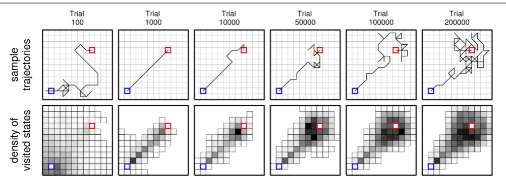
developed by ncMC(0.7) (large center panel) displays a clear pattern in which the mean distance for the last four increases at a greater rate than that of the first four. Behavior generated under ncTD(0) (second from top on the right) shows a simi-lar, but weaker, pattern. Such a pattern is not clearly apparent in behavior generated under the other rules. Other ways of see-ing this pattern are illustrated inFigure 6, which shows sample trajectories (top row) and density of visited states (bottom) for sample trials that achievedsounder ncMC(0.7) at different test points.
The distance metrics in Figure 5 for with-cost rule TD(0) (bottom right) also illustrates the observation made earlier that the bias toward the minimal action sequence for behavior gen-erated under this rule is stronger at early trials (400–2000) than at later trials, even though the rule converges to exe-cuting short action sequences. In addition, the metrics reveal a slightly greater deviation from the direct trajectory for the last four steps of behavior generated under rule ncMC(1) than that for the first four steps. This suggests that additional fac-tors may also influence these metrics. For example, the fact that states visited at latet depend on actions selected at earlier
FIGURE 5 | Mean (across sample trials that achievedso) shortest
distance from the line segment betweenssandsoof the first four steps
after the start of the trial (blue) and the last four steps beforesowas
achieved (red) for learning agents in the grid-world using the different learning rules.Sample trials that did not achievesowere excluded
(otherwise the distance measure would necessarily be shorter for the first four steps because the agents start every trial atss, but they are not
restricted to end every trial atso).Left:schematic illustrating the distance
measures. This schematic uses a continuous trajectory to more-clearly illustrate that the distance measures are based on the first four steps and last four steps of a trajectory; actual trajectories are a series of straight line segments.Center:The mean distance for agents using rule ncMC(0.7) (note the horizontal axis uses a log scale).Right:That for agents using the other rules. Each graph uses the same horizontal and vertical scales and limits.
FIGURE 6 | Sample trajectories (top row) and density of visited states (bottom) (across all sample trials) for learning agents in the grid-world using learning rule ncMC(0.7) at different test points (indicated at the top).For indicating density of visited states, each state
was colored in gray scale: the darker the color, the larger the number of times that state was visited across all sample trials. Statesss (blue) and
so (red) were not colored in, and states that were not visited were not
drawn.
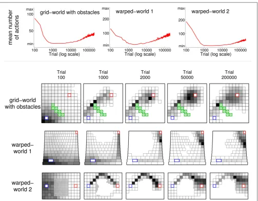
3.4. BEHAVIOR UNDER ncMC(0.7) IN DIFFERENT ENVIRONMENTS
The general pattern of behavioral development observed in agents using ncMC(0.7) acting within the grid-world holds for agents acting within other environments (seeFigure 1) as well. The top row ofFigure 7graphs, in a manner similar toFigure 2, the mean number of actions taken at each sample trial for agents using ncMC(0.7) acting within the grid-world with obstacles (left), warped-world 1 (middle), and warped-world 2 (right). The rest ofFigure 7shows, in a manner similar toFigure 6, the density of states visited for the three environments at different test points for sample trials that achievedso.
Agents using ncMC(0.7) in the grid-world with obstacles dis-covered behavior that used the minimal action sequence (i.e., the shortest trajectory, above the obstacles). Thus, ncMC(0.7) discov-ered the minimal action sequence even when some short-length trajectories (e.g., above and below the obstacles) are not easily
reached from each other (which increases the likelihood of getting stuck in a local minimum).
Agents in warped-world 1 produced behavior that first trav-els east to the border of the world, and then north. Agents in warped-world 2 produced behavior that avoids the middle of the environment by traveling along the upper region of the environ-ment.Figure 7shows that, in the grid-world with obstacles and the two warped-worlds, the minimal action sequence is discov-ered and executed for a temporary but substantial period of time. Also, as with the grid-world, behaviors under the no-cost rules in the other worlds do not converge: with continued reinforcement for an extended amount of time, extraneous actions, beginning at states near the outcome, are executed.
[image:11.595.47.549.285.464.2]FIGURE 7 | Illustration of behavior for learning agents in the grid-world with obstacles and warped-worlds 1 and 2 using learning rule ncMC(0.7). (See Figure 1 for schematics of
[image:12.595.47.551.57.449.2]environments). Line plots (top graphs) follow conventions of Figure 2. Density of visited states plots (rest of graphs) follow conventions of
Figure 6 bottom.
representations were not known, one possible account of such behavior would be that the actions executed at certain locations are simply more costly than actions executed at other locations (e.g., if moving horizontally along the north edge of warped-world 1 was very costly, and moving through the center of warped-world 2 was very costly), and that the learning rule incor-porates these explicit action costs. Our results demonstrate that spatially indirect behavior can also be accounted for with other mechanisms: learning rules that do not incorporate explicit action costs, such as no-cost rules, govern behavior, and the underlying state representation is nonuniform on a spatial level.
We note that the spatially nonuniform state representation also allows for spatially indirect behavior to be accounted for by a learning rule that incorporates temporal discounting of the positive numerical signal received upon achievement of the out-come but does not incorporate explicit action costs. Note also that we do not suggest that a spatially nonuniform state representa-tion prohibits the use of learning rules that incorporate explicit
actions costs. Rather, we demonstrate how similar behavior can be accounted for with different mechanisms.
4. DISCUSSION
numerical signal if the outcome is achieved (which addresses the question “was the outcome achieved?”) along with some combi-nation of explicit negative numerical signals (“costs”) for each executed action and/or temporal discounting of the numerical signals, either of which addresses the question “how well was the outcome achieved?” (Sutton and Barto, 1998).
However, such an account may not apply to all situations in which the minimal action sequence is discovered. In particular, in the process ofaction discovery(Redgrave and Gurney, 2006; Redgrave et al., 2008, 2011, 2013; Stafford et al., 2012; Gurney et al., 2013), the minimal action sequence is thought to be discov-ered by learning mechanisms that focus on the simple evaluation of “was the outcome achieved?” and are driven by a prediction error in the outcome’s occurrence. As discussed inRedgrave and Gurney (2006), biological reinforcement signals in action discov-ery may occur too quickly to evaluate an action sequence beyond an indication of the outcome’s occurrence.
In this paper we demonstrate thatno-costlearning rules, which focus on “was the outcome achieved?” and are more consistent with action discovery than previous accounts, can also discover and execute the minimal action sequence for a temporary yet substantial period of time (Figures 2,7). Under the no-cost rules described in this paper, if the outcome is achieved during a trial, the tendency to execute every action that was executed en route to the outcome is increased, but at a rate that decreases with temporal distance from the outcome (seeFigure 3). In no-cost rules, though, every action that leads to achievement of the out-come is associated with the same measure of behavior. In effect, no-cost rules develop behavior that is similar to behavior devel-oped by rules that focus on “how well was the outcome achieved?” but no-cost rules focus on the simple evaluation of “was the outcome achieved?”
One limitation of no-cost rules as described in this paper is that behavior does not converge if reinforcement continues for an extended period of time (Figures 2, 4,7). This limitation is also consistent with the process of action discovery (Redgrave and Gurney, 2006; Redgrave et al., 2008), which suggests that a separate process that predicts the outcome’s occurrence attenu-ates reinforcement signals as the outcome becomes predictable. (We do not model this proposed process in this paper). If such attenuation were disrupted, e.g., due to disorders of prediction or reinforcement functions, extraneous actions would be developed under no-cost rules, first appearing in close proximity to the outcome (Figures 4–6).
Another limitation, which arises with all scenarios involving learning without external instruction, is that of scaling. The envi-ronments we use (Figure 1) comprise between 100 and 1000 states. It is likely that, as with the more common with-cost RL (Sutton and Barto, 1998) rules we use in this paper, the effective-ness of no-cost rules will decrease if the number of states increases by a very large factor. One area of future research is to augment no-cost rules with techniques used to increase the effectiveness of with-cost rules in very large state spaces. These techniques include the development of state abstractions and behavioral hierarchies (Sutton et al., 1999; Dietterich, 2000; Barto and Mahadevan, 2003; Ravindran and Barto, 2003; Mahadevan, 2010; Osentoski and Mahadevan, 2010; Barto et al., 2013a) which should be applicable,
in principle, to the no-cost rules we use here. We expect any limi-tations from scaling of our no-cost rules to be similar to those of with-cost RL rules.
We also note that, despite a similarity in language, our frame-work is different from that described inFriston et al. (2012). The latter does not invoke notions of optimality or cost because the agent already represents “optimal” behavior (such as the minimal action sequence) as a probability distribution over hidden states that is learned from experience generated by an external supervi-sor. The agent acts to move from low-probability (“surprising”) states that it does not expect to inhabit to high-probability states. Behavior is described in terms of information theoretic measures rather than optimal control.
Below we discuss computational and biological issues related to no-cost rules in behavioral development.
4.1. DIFFERENTIAL RATE OF REINFORCEMENT
In computational RL (Bertsekas and Tsitsiklis, 1996; Sutton and Barto, 1998), the tendency,Q(s,a), to select actionafrom states
is modified with learning rules that modifyQ(s,a) toward some target value (often referred to as thereturn). In many RL-based accounts of human or animal behavior, that target value is a measure of behavior that is influenced by a positive numerical signal (if the outcome is achieved) and also some combination of explicit action costs (negative numerical signals) and/or temporal discounting of numerical signals. (In the with-cost rules described in this paper, there are explicit action costs but no temporal dis-counting). In many tasks and environments, that target value is higher for actions that lead to shorter action sequences and, thus,
Q(s,a) converges to a higher value if it reliably results in achieve-ment of the outcome with a shorter action sequence. In contrast, in the no-cost rules described in this paper, the target value used to modifyQ(s,a) is influenced only by a positive numerical signal if the outcome is achieved; explicit action costs and/or temporal discounting of the signals do not influence the target value. Thus, for tasks similar to those described in this paper,Q(s,a) for all (s,a) pairs converge to the same target value when modified with no-cost rules (see Methods for more details).
Even thoughQ(s,a) for all (s,a) pairs converge to the same value in no-cost rules, the minimal action sequence is discovered and executed for a substantial amount of time with (Figures 2,
While there are likely many behaviors in which learning mech-anisms associate behavior with a measure that is influenced by explicit action costs and/or temporal discounting, the central nervous system has multiple learning and control schemes at its disposal (Milner et al., 1998; Yin et al., 2008). By modifying differentQ(s,a) at different rates toward the same target value, as opposed to modifying differentQ(s,a) toward different tar-get values, no-cost rules are able to discover and execute the minimal action sequence (temporarily) through different mech-anisms and with different types of information than with-cost rules.
The differential rate of reinforcement can be accomplished with a decaying eligibility trace (Pavlov, 1927; Sutton and Barto, 1981, 1998; Klopf, 1982; Wörgötter and Porr, 2005) in Monte Carlo (MC) rules, which deliver reinforcement signals only at the end of a trial (such as rule ncMC(0.7)) when the out-come is achieved (Sutton and Barto, 1998). In Lecture III of his famous account of conditioned reflexes (Pavlov, 1927), Ivan Pavlov discusses how thetraceof a conditioned stimulus (CS) allows behavior in response to the CS to be modified by an unconditioned stimulus (US, which produces the reinforcement signal) that occurs at a later time, and how the effect of rein-forcement is weaker as delay between CS and US increases. Eligibility traces play a prominent role in several computa-tional models of brain function (such asSuri and Schultz, 1998; Wörgötter and Porr, 2005; Izhikevich, 2007; Vasilaki et al., 2009; Chersi et al., 2013) and are used to describe several experi-mental results (Markram et al., 1997; Bi and Poo, 2001; Pan et al., 2005). They may be implemented in the brain through persistent neural activity (Goldman-Rakic, 1995; Curtis and Lee, 2010) or, as has been suggested in some modeling stud-ies (Houk et al., 1995; Suri and Schultz, 1998), intracellular processes.
It is unclear if the influence of eligibility traces can extend to actions executed many time steps before the outcome in biological systems. However, the “bootstrapping” nature of tem-poral difference (TD) learning rules (Sutton, 1988; Sutton and Barto, 1998), in which intermediate states that predict a rein-forcing event themselves become reinrein-forcing, enables actions that are executed many time steps before the outcome to be rein-forced. This paper demonstrates that TD rules also, in effect, reinforce actions proximal to the outcome at a faster rate than actions distal to the outcome. Thus, no-cost TD rules (such as ncTD(0)) can also discover and execute the minimal action sequence for a substantial period of time, even without eligi-bility traces. Recent experimental results (Wassum et al., 2012) demonstrate that dopamine (DA) release (thought to communi-cate reinforcement signals,Wickens et al., 2003, also discussed later in the Discussion) is propagated from proximal to dis-tal actions in rats engaged in a operant conditioning task that requires a sequence of two separate actions in order to achieve an outcome.
Of course, the differential rate of reinforcement on which no-cost rules rely is not restricted to no-no-cost rules. MC rules and TD rules using with-cost measures with or without eligibility traces can easily be implemented (Bertsekas and Tsitsiklis, 1996; Sutton and Barto, 1998). The no-cost rules described in this paper allows
us to more clearly demonstrate the functional mechanisms by which differential rates of reinforcement help shape behavioral development.
4.2. DOPAMINE ACTIVITY
In order for behavior developed using no-cost rules to con-verge with extended experience, a separate process must attenuate reinforcement signals. Reinforcement signals in the brain are thought to be communicated by phasic DA neuron activity (henceforth referred to simply asDA activity). Experimental stud-ies (Ljungberg et al., 1992; Schultz et al., 1993, 1997; Horvitz, 2000; Redgrave et al., 2011; Schultz, 2012) have shown that sensory-evoked DA activity attenuates with repeated presenta-tions of the sensory stimulus. If mechanisms similar to no-cost rules participate in behavioral development, such participation provides a functional-level teleological explanation for why DA activity attenuation occurs: DA activity that is not attenuated by a separate process would result in prolonged reinforcement and consequential degradation of performance.
This interpretation is different than that in which DA activ-ity is accounted for solely by the learning rule, i.e., in which the rule accounts for both an increase in DA activity (reinforce-ment) and its subsequent attenuation (Houk et al., 1995; Schultz et al., 1997). In this case, if the outcome can be achieved in many ways, it is necessary that the target value toward whichQ(s,a) is modified represents a measure of behavior that is higher for actions that achieve the outcome in some “better” way than other actions that achieve the outcome (such as the with-cost mea-sures described in the Methods). Otherwise, extraneous actions will occur. Most studies describing DA activity in such terms use fairly simple tasks (e.g., the outcome is biologically rewarding and is dependent on only one or two actions) to investigate how DA activity propagates from the outcome to otherwise neutral stimuli or actions that precede the outcome (Schultz et al., 1997; Schultz, 2012; Wassum et al., 2012) rather than how redundancy is resolved.