Finite element error estimates for nonlinear elliptic problems of monotone type

OF MONOTONE TYPE

by

-S.-S. CHOW

A thesis submitted to the

Australian National University

STATEMENT

The proof of Lemma 3

.

1 was suggested by Frank de Hoog.

Elsewhere

1n

this thesis, unless otherwise indicated, the work is my own

.

~ / / ( _

-ACKNOWLEDGEMENTS

The work for this thesis was undertaken in the Department of Mathematics in the Faculty of Science of the Australian National

University. I would like to thank the heads of the department, Dr N.F. Smythe, Professor N.S. Trundinger and Dr P.J. Cossey, for their general support and acknowledge the financial assistance provided by the

Australian National University.

I am greatly indebted to my supervisors Bob Anderssen and Frank de Hoag for their constant encouragement and helpful advice. Their interest and concern with my work has been most invaluable. I thank them deeply for their effort in providing me with the best possible supervision and for their many constructive criticisms of this thesis. I also wish to thank Bob Anderssen for catching numerous grammatical errors that appeared in the draft.

Without the support and sacrifice of my family, i t would not be possible for me to complete this study. I am most grateful to them for their support and perseverance with the many hardships. I would especially like to thank my mother for encouraging me to study abroad so that I may have the opportunity to develope a greater appreciation and understanding of the land and people in this country.

During the past three years, I have benefited greatly from discussions with staff and fellow students. The many discussions I had with others while attending conferences and seminars are also valuable.

ABSTRACT

In this thesis, we examine the order of convergence of finite element approximations to some nonlinear elliptic problems of monotone type. This is determined by establishing error estimates in the 'energy' norm for the approximations. The nonlinear problems we are interested in arise in many practical situations. Examples from blast furnace gas flow, magnetostatic

distribution and nonlinear seepage flow are discussed in some details. In Chapter 2 we show that a class of second order boundary value problems of divergence form with gradient nonlinearity may be formulated variationally, and, in an abstract setting, as an operator equation, if the nonlinear coefficients of the equation satisfy certain conditions. Under

these conditions the operator turns out to be monotone. In Chapter 3 we introduce the concept of strong monotonicity and T-continuity and

demonstrate the relation between strong monotonicity and convexity. We then prove the strong monotonicity and Holder continuity of the operator

introduced in Chapter 2. The well-posedness of the boundary value problem is then shown by establishing the unique solvability and stability of the problem.

In Chapter 4, after showing how error estimates for finite element approximations maybe obtained in an abstract setting if the associated

operator is strongly monotone and T-continuous, we proceed to derive error estimates for the class of nonlinear problems discribed earlier and examine the order of convergence of the finite element approximations under the assumption that the (weak) solution satisfies only a weak regularity

condition.

Hilbert space, it is of interest to consider the optimality of the order of convergence in other cases. In Chapter 5 we establish the conditions under which a class of nondegenerate equations, including Ergun's equation and nonlinear seepage flow equations, can be shown to have the optimal order of convergence. We also examine the problems of error estimation in

W1' 2-norm and for a class of problem solvable in the W1'P-Sobolev space with p > 2 .

In Chapter 6, we use the method developed earlier to establish a

variational formulation for a class of nonlinear vectorial boundary value problems and to derive error estimates for the finite element approximations.

In the last chapter we discuss a direct method for solving a class of one dimensional problem and present some results from numerical

STATEMENT .. ACKNOWLEDGEMENTS ABSTRACT

TABLE OF CONTENTS

CHAPTER 1: NONLINEAR PROBLEMS 1.1 Introduction

1.2 Formulation of Ergun's equation 1.3 Nonlinear seepage flow

1.4 Magnetic field analysis

(i)

(ii)

(iii) l l 8 11 14

CHAPTER 2: VARIATIONAL FORMULATION AND FINITE ELEMENT APPROXIMATIONS 18

CHAPTER 3:

CHAPTER 4:

2.1 Function analytic preliminaries ..

2.2 Properties of associated functions 2.3 Variational formulation ..

2.4 Finite element approximations ESSENTIAL INEQUALITIES

3.1 Introduction

3.2 Monotonicity and convexity

3.3 Holder continuity and strong monotonicity 3.4 Well-posedness

ERROR ESTIMATION I

4.1 Abstract error estimates 4.2

w

1'P-error estimates

4.3 Equations with implicitly defined coefficients 4.4 Weaker regularity assumptions

CHAPTER 5: ERROR ESTIMATION II 5.1 Introduction

5.2 Optimal estimates for nondegenerate equations 5 . 3 Wl,2 -estimates or linear triangular . f . . e l ements 5.4 Equations in W1'P(~) with p

~

2

CHAPTER 6: THREE DIMENSIONAL MAGNETOSTATIC DISTRIBUTIONS 6.1 Variational formulation

6.2 Error estimations

CHAPTER 7: NUMERICAL SOLUTION OF NONLINEAR PROBLEMS ..

REFERENCES

7.1 7.2 7. 3

Direct method for one dimensional problem Numerical results

Concluding remarks

CHAPTER

1

NONLINEAR PROBLEMS

1.1

Introduction

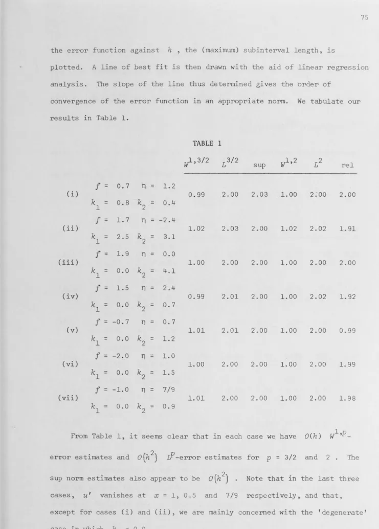
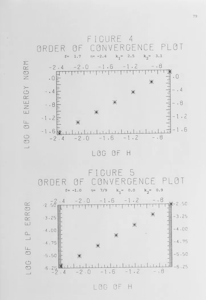
Whenever an approximating process is utilised to obtain an approximate

solution, it is appropriate to provide an error estimate (that is, a measure of the proximity of the approximation to the actual solution). This error estimation is especially important in numerical schemes because, in addition

to generating relevant technical information, it may also be used as an

indicator of the efficiency of the algorithm used and to provide valuable insight whenever one needs to modify the approximation procedures. For

example, error estimates play a key role in the analysis of grid refinement techniques. In this thesis, we construct error estimates for finite element approximations of certain nonlinear boundary value problems that can be

analysed using monotone operator theory.

Throughout this thesis, let be a bounded open domain in

n

> l , with Lipschitz boundary 3S1 = r

0 u f , where r0 and f are disjoint and meas(r

0) is strictly positive. Let

n

be the unit outward normal vector on r . The class of problems that we are mainly concerned with takes the form

-V •

(k

(x,

I

Vu(x) I Vu(x)) -

-

~g(u(x)) + f(x) in _{St '} (la)

u(x) -- (j)(X) on ro (lb)

'

-k(.x, IVu(x)l)vu(x) • n = n(x) on r

'

( le)

where f g

' ' (j) and

n

are functions with various properties, which will be discussed later. The function k E C(St x IR+) is assumed to be positive and for almost every x E St ,

k(t)t

is a strictly monotone increasing

value problem (la-le) must be elliptic, while the latter is needed to ensure

the applicability of the method of monotone operators.

Such types of boundary value problems arise naturally in many real life situations. Examples which arise in areas of blast furnace operation, non-linear seepage flow and turbogenerator design, are discussed in the

remaining sections of this chapter, along with the formulation of the

associated boundary value problems .

Even for the simplest linear cases, it is virtually impossible to obtain solutions in closed form when

n

is not one dimensional.

Consequently, some form of approximation must be used to determine the behaviour of the solutions. One possibility is the

finite element method.

Its appeal over other numerical methods is connected directly with the

divergence structure of (la), the existence of variational form for (la-le)

and the flexibility of the finite element method in dealing with complex

geometric domains.

If the finite element method is used to construct approximations to the

solutions of (la-le), then it is necessary to examine the quality of such

approximations. For linear equations , it is well known that the finite

element approximations yield the best approximations to the (weak) solution

of the problem in the energy space ([8], [28], [43]). The situation is not

so clear cut when nonlinearity is introduced. Even for one dimensional problems, it is not in general possible to characterize the approximations

along the lines used for linear problems.

Nevertheless, there exist many problems for which one can use the best approximation characterization for finite element approximations . In almost all cases, an error inequality is established which yields an upper bound

of linearity in linear problems. For nonlinear problems , an important tool in establishing the error estimate is the method of monotone operators.

Once such inequality is derived, it only requires one to draw on results from approximation theory to obtain specific properties of the error.

In [9], Ciarlet, Schultz and Varga studied the semi-linear two point boundary value problem

.I (

-1) j + 1

z:P

'P

. (

x)

zl

u ( x

0 -

f ( x , u ( x)) , O < x < l , n > l ,

J=O ~J

j

with boundary conditions

D - d

dx ' O < k < n-1 .

A

By considering the finite dimensional approximation

WM

as a projection of

the classical solution ~ on the finite dimensional subspace

SM

with

respect to a subspace dependent inner product, they obtained proofs of

convergence of polynomial, piecewise polynomial and spline approximations. 00

These results are derived from the L -norm estimates they constructed for the approximation and its derivatives. They proved that

llw-~

11

y (2)

where

K

and

C

are constants which can be explicitly determined a pri,or~ , y is a lower bound for f (x,

u)

u and the norm

II

·

lly

i s defined by

2

Il

(

n ( · 2

J

2

1

·

llw

II

=

.I

p . ( x) (

lf

w

(

x)) +

yw (

x) dx .

y O J=O J

By letting

SM

be the polynomial, piecewise polynomial and spline subspace

in turn, and utilising results from approximation theory for these subspaces when the norm is

11

•

lly

,

_{the required} L 00 -error estimates follow from (2) .

Note that, for higher dimensional problems , the first inequality in (2) is

continuously embedded in L00

(n)

when

n

c IRn with n

~

2 .

In a later paper [10], Ciarlet

et al

obtained abstract error estimates

for some nonlinear boundary value problems associated with a finitely

continuous , bounded and strongly monotone operator defined on a reflexive

Banach space. However, the operators associated with many important

problems do not possess these assumed properties. More specifically as we

shall see later, many interesting operators are unbounded in the Banach

spaces on which they are defined.

Noor and Whiteman [34] also derived abstract error bounds for a class

of semilinear elliptic boundary value problem with the associated nonlinear

operator being antimonoton2 and Lipschitz continuous in the corresponding

Hilbert space. In the same paper they demonstrated the relation between the

antimonotone operator and a convex nonlinear functional. This connection is

conceptually important in much of the study of boundary value problems

involving the application of monotone operators.

Glowinski and Marrocco [17] studied (la-le) with

(3)

where s > 0 ,

S

> l > a are known constants, in a Hilbert space setting.

Using the fact that

k(t)

is a strictly increasing continuous function of

t ,

they proved the convergence of the finite element solutions but did not

derive any error estimate. Xie [48] also studied (la-le) in a Hilbert space

setting for a general

k(t)

and derived results which correspond to those

of oor and Whiteman. Xie noted that the strictly increasing property and Lipschitz continuity of

k(t)t

may be exploited to prove the strict

monotonicity and Lipschitz continuity of the operator associated with the problem and to obtain an error estimate for the finite element approximation. For

k(t)

in (3) it is not difficult to see that

(k(t)t)'

is bounded

From the discussion above it is clear that the method of monotone operators is of considerable importance in establishing the desired error bounds. We recall that monotonicity is intimately related to convexity, and it is natural to expect that the variational functional associated with

(la-le) is convex in some appropriate function space if the operator

corresponding to (la-le) is monotone. In Chapter 2, we examine a variational formulation for (la-le) and introduce the notions of weak solutions and

finite element solutions. We then study in the first part of Chapter 3 the concept of strong monotonicity and its relation to coercivity and the

increasing property of a Gateaux differentiable functional.

Glowinski and Marrocco [18] studied in some detail the finite element solution of the degenerate boundary value problem

u

-

0 on 3~ ,

and proved that the corresponding abstract operator A is strongly

( 4-a)

( 4-b)

monotone. They also showed that for l < p < 2 , A is H 0

older continuous

with exponent p - l , and, for oo > p ~ 2 , A satisfies an inequality of the form

II

A

u-

Av

II*

<

yll

u-vll

c

II

ull

+II

vii

)p-2

when _y is a positive constant and

11

•

11

,

II·

II*

are norms on appropriate spaces . These results concerning the boundary value problem (4-a-4-b) are important in that when p # 2 , the operator equation cannot be studied conveniently in a Hilbert space setting and that when p E ]l, 2[ , the

operator A is unbounded in its natural space of definition. Consequently, none of the results in the works mentioned earlier on may be used to

establish error estimates for approximate solutions of (4-a-4-b) .

other problems we must employ other properties of

ta

to complete the

proofs.

In §3. 3 we replace this homogeneity property with the condition that

k(t)t

be strictly increasing and Holder continuous with exponent p - 1 ,

1 < p S 2 . Thus, by extending the ideas of Xie and utilising some of the techniques of Glowinski and Marrocco, we obtain inequalities similar to those mentioned earlier. With the aid of these inequalities, the well posedness of (la-le) and the unique solvability of the finite element solution is established.

In Chapters 4 and 5, we are mainly concerned with deriving error estimates for finite element approximations of (la-le). After describing the general procedure of obtaining error estimates in an abstract setting, we utilize the various inequalities derived in Chapter 3 to obtain

w

1'P-error estimates for the finite element approximations of (la-le). As

we shall show below, there exist· situations where the function

k(t)

is not known explicitly and we only have at our disposal a function

l(s)

such that

t

=

l(s)s

if and only if

s

=

k(t)t

.

We shall examine how error estimates may be obtained in such a case. It is also of interest to study the behaviour of the error under weak regularity assumption and this is done in the last section of Chapter 4.

When p < 2 , the result obtained in Chapter 4 is not optimal in the sense that the derived order of convergence of the finite element

approximations is less than those in the case of linear equations. By

d · h d d b ·

w

1' 2 · f h · · f

a apting a met o use too tain -estimates or t e minimal sur ace equation [20], we prove that one obtains the optimal W1'P-estimate for

k(t)

bounded above by some constant , in addition to certain regularity

assumptions. We also show, how one may, in an analogous way to [20], obtain

and regularity assumptions, for two dimensional problem using linear

elements . The case when the solution space of the boundary value problem

(la-le), is in

W

1

'P(~)

with p > 2 is then considered.

In Chapter 6 we use the techniques developed in Chapters 2, 3, 4 to

study a class of nonlinear vectorial boundary value problems of the form

curl(~Clcurl ul) curl u) -

j

in

A,

div U - 0 in

A,

and

curl U •

n

-

O on

8A,

where A is a bounded open simply connected domain in IR 3 , and

n

is the

outward normal on the boundary

8A.

An example of this type of problem

arises in the analysis of a three dimensional magnetostatic field

distribution in a turbogenerator (see §1.4). After introducing the

appropriate function spaces which enable us to construct a variational (or

weak) formulation of the problem, we derive error estimates for the finite

element approximations and show the well posedness of the boundary value

problem.

In the final chapter we examine a direct method for solving (la-le) in

one dimension with minimal assumption on

k(t)

and present the result of

some numerical experiments for Ergun's equation in one and two dimension.

In the remaining sections of this chapter, we consider some actual

problems which can be formulated in the form of (la-le). Besides providing

motivation, such examples also serve two purposes - the form of the

functions

k(t)

derived enables us to extract information to further our

mathematical intuition and the physical aspect enables us to develop further

insight by drawing on experimental data when necessary. We begin our

1.2

Formulation of Ergun's equation

BLAST FURNACE PROCESS

The production of pig iron from ferrous ore by blast furnaces has a relatively long history compared with other metal smelting processes currently in use. The first blast furnaces, having sufficiently high

temperatures to melt iron, came into existence in Germany and Belgium in the fourteenth centruy. Since the introduction of preheated blast at the

beginning of the nineteenth century, various modifications and adjustments in scale, design and operation practice have been under investigation up to the present day. However, the basic structure of the blast furnace has

changed very little in the course of time. This is a direct consequence of the fact that there is still very limited information about the extremely complex chemical and physical processes occurring within the furnace.

General details about blast furnace processes may be found in [4].

The blast furnace is a packed bed reactor. In order to optimise the design of the reactor and to improve the operator's procedures so ·as to achieve a better performance in terms of cost and productivity, it is necessary to have a good understanding of the flow distribution in packed beds having spati ·ally non-uniform resistance. The experimental approach has two major disadvantages. Firstly, a small scale model does not provide a satisfactory representation of the furnace. For example, it is very

difficult to achieve the high termperature associated with the operation. Secondly, the cost of obtaining realistic information from commercial

furnaces is extremely high. This is especially true, when the investigation involves the dissection of a quenched blast furnace ([21], [22]).

By comparison, the mathematical modelling approach does not suffer from such disadvantages. As long as a good model is available, it is possible to obtain valuable information at a reasonable cost. In 1952, Ergun [14]

his observation that losses in pressure are caused by simultaneous losses in

viscous and kinetic energy. While Ergun's law is of great value, it

represents, due to certain underlying assumptions, an over simplification as

it does not allow for non-uniform flow. In most practical applications , the

non-uniform packing of the reactant particles leads to the so called wall

effect which in turn causes non-uniform flow . In order to overcome this

difficulty, Stanek and Szekely [42] proposed a vectorial differential form

of Ergun' s law.

ERGUN 'S LAW

Stanek and Szekily proposed that Ergun's law for incompressible fluid

flow, with its validity confined to the direction of flow and to an

infinitesimal length of the bed, be given by

(5)

while for compressible flow , without any restriction on its validity, by

(6)

where p is the pressure,

V

the superficial velocity and

G

the mass

velocity. The parameters of resistance and are given by

and

where µ denotes dynamic visocity,

s

porosity, d particle diameter and

p density.

We assume that the temperature profile within the reactor is known, and

that the compressible fluid passing through the packed bed satisfies an

equation of state of the form p/p =

F(T)

,

for some known function

F

of

the temperature T (for example, the perfect gas law) . Thus we may regard

variables in the region of interest.

We now show that Ergun's law, when coupled with the continuity equation,

is equivalent to a second order elliptic partial differential equation in divergence form. The continuity equations for incompressible and

compressible fluid flow in packed bed reactors are

and

respectively, where

V·V = f(x) - g(x, p)

2

V • G = f(x) - g (x, p )

f : S1 -+ IR and g :

n

X IR ( or

(7)

(8)

+

n

x IR ) -+ IR are known functions and represent (possibly pressure dependent) source and sink terms within the packed bed.

Consider the case when the fluid is incompressible. Taking the modulus of (5) and recognizing that both

f

1 and f :2 are positive, we have, after

solving a quadratic equation and taking only the positive root.

( 9)

Using (5), (7) and (9) we get

(10)

A similar algebraic manipulation with (6) and (8) yields an equation of the same form as (10) with

respectively.

and _p 2 replacing and _{p '}

To complete the formulation of the problem, we examine the boundary

conditions . Let us assume that, along

r

0 , the pressure is prescribed by a

continuously differentiable function ~ and that, along the remaining

portion of the boundary, the normal component of the superficial velocity (of the mass velocity in the case of compressible fluid) is given by a known

the Neumann boundary condition is transformed to

(11)

Letting

u

= p - ~ , it is clear that equations (10) and (11) retain

essentially the same form while the inhomogeneous Dirichlet boundary

condition on p becomes a homogeneous one on

u

along

r

0 It is clear

that, for the compressible fluid case, the boundary conditions may be dealt

with in a similar manner and analogous expressions are yielded if the

substitution _u = p 2 - ~ 2 is used.

Letting k

1, k2 ,

u

and ~ stand for

f

1/2,

f

2, p and ~ respectively

if the fluid is incompressible or for _{and ~} 2 _{if the fluid}

is compressible, we see that a mathematical formulation of the steady s·~ate

gas flow within a blast furnace is given by

where

Clearly k

-V• (k(

I

Vul )Vu) - f(x)

u(x) - ~(x)

-k(IVul )Vusn -

n(x)

g(x, u) in St ,

on

ro '

on

r

k(t) =

~l

+

v

ki+k2t

Tl .

is a positive continuous function on St x IR+ _and

(12a)

( 12b)

(12c)

(13)

(14)

is a strictly increasing function of

t

.

Therefore (12a-12c) is of the

type (la-le).

1.3 Nonlinear

seepage

flow

We now reexamine Ergun 's law for seepage flow. Such a consideration is

porous medium. Darcy's law is commonly adopted for describing pre-limina or

creeping flow in which inertia effects are negligible [3]. If viscous

dissipation dominates and the Reynolds number is small (for example ,

Re~ 1.5), then we may set and to zero in (5) and (6) respectively.

Ergun's law may then be regarded as a variant of Darcy's law and (12a-12c)

-1 ( -1 -1)

reduces to a familiar linear problem with

k(x, t)

.

=

2k

1 .=

f

1 or g1 .

On the other hand, if the flow is dominated by turbulence dissipation and

large Reynolds number (for example , Re~ 150), we may drop the viscous term

in Ergun's equation. Assuming that

g(x, u)

=

0 , we may write (12a) as

( 15)

Clearly, when k

2

(x)

-

constant , (15) is a special case of (4a) with

p - 3/2 .

Equations of the type (15) or (4a) also arise naturally in modelling

the flow of a liquid or gas through a porous medium satisfying Missbach's

law [47] which provides a relationship between velocity and hydraulic

gradients :

( 16)

where is the velocity in the direction _{s '} h is the hydraulic head

and c , n are constants .

There exists another seepage law which describes the nonlinear behaviour

of laminar and turbulent flow. Forchheimer's law [47] is given by

ah

2

as - aq s + bq s '

and resembles the vectorial differential forms of Ergun's law for

incompressible fluid first proposed by Stanek and Szekely [41] :

~

-dX

~

-d

(17)

(18a)

Subsequently , it was pointed out that (18a-18b) are not invariant to

coordinate transformation and hence formally incorrect [38]. Thus one may

modify (17) to a form similar to (5) when the fluid flow under consideration

is isotropic. (The above comment is also applicable to the Missbach law.)

An example of such a modification appears in the study of glaciology by

Pelissier [37], which gives rise to (4a) .

Since the continuity equation may be written as

V

•

q =

f(x)

-

g

(x,

h) in Q (19)

with source or sink term

f(x)

-

g(x

,

h)

and velocity q , it is clear that the equation of divergence form in h resulted by coupling the modified

equation ·of (17) and (19) is of the same form as (12a).

More generally, one may consider the nonlinear seepage law [35]

(20)

where n ~ 0 is a constant and a , b are positive continuous functions of

the spatial variables in the region of interest. In order to derive an

equation of the form (la) we first note that the function

Z(s)s

=

(a+bs1'2)

s

mapping to is strictly increasing in S , and hence possesses a

strictly increasing inverse function

k(t)t

, that is,

.

t

=

Z(s)s

if and only if s =

k(t)t

.

Thus we may write (20) as

q =

k(!Vhl)Vh

.

(21)

For n

t

O or l , it is very difficult , if not impossible, to derive

k(t)

explicitly. Nevertheless, a numerical evaluation scheme may be used

to determine

k(t)t

economically in the course of computing a solution to

the boundary value problem modelling the flow . The boundary value problem is obtained by combining (19) and (20) as well as appropriate boundary

l

.

4 Magnetic

field analysis

One advantage of mathematical modelling over others is that very often the same model may be used to describe vastly different physical phenomena.

One such example is the wave equation. In this section we provide yet another illustration of the above statement by showing how (la-le) can be used as a model for the magnetostatic field distribution in turbogenerator or electromagnet design problems . In the process of modelling such problems another type of boundary value problem arises, which will be studied in more

detail in Chapter 6.

In order to optimise design and to ensure reliability of electrical

machinery and devices an accurate prediction of the magnetic field

distribution in their active region is required. The presence of complex geometries and material discontinuities invariably exclude the possibility of obtaining an analytical solution. The finite element method is well

suited to dealing with such complications.

Let A be a simply-connected bounded open domain in IRn , n

~

2 ,

with smooth boundary 8A and let n be the outward unit normal to aA . By assuming that the permeability µ is a single-valued scalar function

(that is, istropic material and ignoring hysteresis effect) and the source function is represented by a volumetric current density distribution in

ideal conductors carrying current, the stationary magnetic field distribution in A lS given by the Maxwell's magnetostatics equations

curl H -- J (21a)

'

B

-

_-

µ.H

_{( 21b)}

'

div

B

-_{- 0 (21c)}

'

where H is the magnetic field intensity, J the current density vector, and B the magnetic induction (all in appropriate units) .

The solenoidal vector

B

may be represented by a potential vector

A

B

= curl

A.

₍₂₂₎ Letting V be the magnetic reluctivity (inverse permeability), i t is clear that (2la-2lb) and (22) yield

curl(V curl

A) -

J in

A.

(23a)

The reluctivity is a function of

IBI

and for ferrous material is

highly nonlinear. It is usually available for interpolation of experimental cata as the

B

-

H

curve. Some typical forms of

v

are

(i) with a - 4.5 X 10-4 ,

+4

S

=

2.2 x 10 and s

=

8 for the rotor in a turbo

-alternator, and

s -

5.16 x 10-4 ,

C

=

0.176 ,

T

=

8.76 x 103 and

a -

5. 42 as a typical set of values.

In both cases µ

0 = 4TI x l0-7

MKSA.

Clearly, if A is a vector function satisfying (23a), then, for any continuously differentiable function

X,

A

+

grad

X

is also a solution of (23a) . Thus, to ensure uniqueness , we impose the normalising condition on

A :

div

A

=

0 in

A.

(23b)

If we assume the magnetic field outside the machine or device is negligible,

we obtain the boundary condition

curl A• n = 0 on 3A . (23c)

Equations (23a-23c) may be regarded as a boundary value problem. This

problem is considered in detail in Chapter 6 .

We now consider the case when the magnetic vector potential and the

current density vector have only a component in the 2-direction, that is,

and

J = (0, 0, g)

with

u

=

u(x,

y)

and

g

=

g(x, y)

.

Clearly (23b) is satisfied identically

and, noting that !Bl - !curl

Al

=

I

grad

ul

,

(23a) gives

-V

•

(vC!Vul)Vu)

= g in A

The boundary condition (23c) is satisfied if

u -

o

on

aA

.

Note that we use the same symbols

A

and

aA

for the two dimensional

analogue of the original region and boundary respectively. Obviously

(24a)

(24b)

(24a-24b) is a special case of (la-le) since v(t)t is an increasing

.

.

function of

t

E IR + , as can be seen from the

B

-

H

curve :

[image:23.772.8.754.19.1073.2]

B

FIGURE 1

Returning to the fully three dimensional case, the solution of the

magnetic vector potential A requires computation for the three components

of

A,

and is thus rather costly in terms of execution time and memory

requirement . It is natural then to seek an alternative approach whi ch is

more economical, computationally speaking. The method of scalar magnetic

potential provides a competitive approach to the solution of (2la-2lc) . From Maxwell' s theory we know that the current density vector is

solenoidal, so by letting

J = curl H

0 for some vector H

0 , with no restriction on its divergence , we may represent H by the sum of its irrotational and rotational parts:

H

= - grad¢+

H

0

where ¢ is termed a reduced scalar potential.

(25 )

Suppose now that a suitable H

0 satisfying (25) is chosen. This may

be obtained by evaluating the integral

1

J

j

C

r'

) C

r- r'

)

dv

,

H

0Cr ) = -_4n

_v

_'

I

_r-r'

I

₃ (27)

or by the method described in [29]. Noting that the representation (26) is

still not unique , we impose the normalising condi t-ion

{

¢(x)dx

= J St

0 .

Substituting (26 ) in (21b) and (21c) we see that

div(µ(I H

0 + grad ¢I )

(H

0 +grad¢)) - O in

A

.

(28a)

( 28b)

From the

B

-

H

diagram it is clear that µ(t)t is a strictly

increasing function of

t

~ 0 , so (28a-28b) is strongly related to

(la-le) . The problem (28a-28b) is however a purely Neumann problem, with

boundary condition

B •

n

-

(

H

0 +grad¢) •

n -

b(x)

on

8A,

(28c)

for some given function

b

(

x

) .

We will see later that the results obtained for (la-le) also hold for

(28a)-(28c) with minor modification. Moreover, the computational cost for

solving (28a)-(28c) is much less than that for solving (23a-23c) . However,

we must point out that the computational cost for obtaining H

0 is q ite

substantial and so this scalar potential approach is not always superior to

the vector potential approach. In fact , numerical investigation using the

latter approach is becoming quite popular among the engineering community

CHAPTER 2

VARIATIONAL FORMULATION AND FINITE ELEMENT APPROXIMATIONS

2.1

Function analytic preliminaries

The practical problems discussed in the previous chapter show that it is important to obtain solutions , or at least approximations to solutions, of (l.la-1.lc). To do this we shall consider (l~la-1.lc) in a variational setting and formulate the problem as one in functional minimization . This

enables us to introduce the notions of weak solutions and finite element approximations in a natural manner. We begin by stating some relevant

definitions , notations and results to be used later.

IR+

We use _{to denote the set of all nonnegative real numbers. For any}

p

t

O , and

inequality:

n .

x, y E IR , n > 1 , we have the _p-triangle

where

f1 if 0 < p < - l

'

C

-tp-1

-p

if 1Sp< 00 _•

Clearly, for O < p S 1 , we also have the inverse p-triangle inequality

Let

m

be a nonnegative integer and p E [l, co] . If

O

is an open

set in IRn , we the norm

_II

_·

_llm

_,p

denote by given by

llulip

m,p

the usual Sobolev space equipped with

on 0 For

n

C IRn _{(see §1.1), we define V}

to be the closure of D(rt u r) for the ll • 11

1 ,p norm. For each p > l , one can find r E IR and a unique trace map R

the trace embedding

R(W

1

'P(rt))

~

Lr(r

0

)

holds

[23].

Thus, a characterization of V is

V

=

{u

E

w

1,Pcni

[Ru=

0

a

.

e

.

on

ro}

,

Using the Poincare inequality it is clear that the seminorm

(1)

is in fact a norm on V and is equivalent to the

II

·

II

_l,p norm _.

In some situations , our assumptions on

n

do not hold. When meas(r

0)

is zero, we set

v

=

{

u E

w

1 ,p

Cn l [

In

udx

=

o}

.

In this case, the seminorm

II·

II

is again a norm on V .

The space V equipped with the norm (1) is a reflexive, separable and uniformly convex Banach space for p

E

]l, oo[

[23].

We shall denote the dual space of ( V,

II

·

II)

by ( V* ,

II

·

II*)

and the pairing ( • , • > : V* x V -+ IR by

< f, u

> -

In

fudx

for every _{f E}

_V*

and _{u E}

_V

_.

Also, for p > 1 and _pq

₌

_p + q

'

let

II

•

II

r

*

denotes the norm on the

dual space

_Z*

of

z

=

w

1 /q,Pcr) and (

.

'

.

)

r

'

the

with its dual. For each

u

E

Z

and

v

E

Z*

,

we set

< V' u

>r - Ir

uvdY .

From now on, unless otherwise indicated, we always assume p E ]l, 2] .

We shall also use C to denote a generic constant which is not necessarily the same in each of its appearances .

2.2 Properties of associated functions

We now define the properties which the functions k , g,

f,

q> and

n

will be assumed to satisfy. As stated in §1.1,

k(•,

•)

is assumed to be a positive continuous function on S1 x IR+ and, for a.e .

x

E S1 ,

k(x,

•) •

is a strictly increasing function on IR+ • We follow the convention that whenever

k(•)

i s used it is meant to represent the function

k(x,

•)

for a .e . x E S1. In general, we do not assume that

k(t)

is bounded above. However, the function

k(t)t

is assumed to vanish at the origin and

satisfies the following conditions for some p E ]l, 2]

(i) for all

t

ER+,

where a

1 > 0 , a2 ~ 0 are constants independent of

t

,

(ii)

k(t)t

is Holder continuous with exponent p - 1 , that is,

there exists a constant

y

> 0 , independent of

t

and s , such that

lk( t)t- k(s)sl < Yl t-slp-l for all

t

,

s E IR + ;

(iii)

k(t)t

is continuously differentiable for all

t

> 0 and one can find constants

that

K > 0

l - ' K 2 > O and C 1 > 0

As a consequence of (3), and the simple inequality

for all

t

> 0

'

such

(2)

( 3)

(4)

( 5)

it is easy to show that

k(t)t

-

c

1

(x

1+K2

t

2

_-P)t

nonnegative function for all t > 0 . Then we have

(6)

Obviously, the monotonicity of

k(t)t

does not imply monotonicity for

k(t)

.

However, the converse implication holds . When

k(t)

is monotone, it is not unreasonable to expect that those results, established by

exploiting the various properties of

k(t)

described above, will remain valid under a sli ghtly weaker condition on k . This is indeed the case .

As we shall see later, if

k(t)

is monotone increasing, we may i gnore (iii) above and only require

k(t)

to satisfy (6).

As an illustration , consider Ergun's problem (l.12a-l.12c). In this case ,

k(t)

_-

-

₍

_kl

+J

_k~

_+k2trl

_and

_k(t)t

-_-

_[

_j

_k~

₊

_kl

_-k

1)

_/k2

_.

It is easy to check that

k(t)t -

_- 0 at

t

-_{- 0 and conditions (i)-(iii) are}

A A

satisfied with p - 3/2 _al - y

₌

_k2

_a.2 - ₀

Kl -

k

K2

=

k

and

-'

-

'

-

'

- 1

'

2

A

~k

k

.

C -_- where

k.

> 0 and > _{0 are respectively the upper and lower}

'

-1 2 1,, 1,,

bounds of k . ,

1,,

.

i, - 1, 2 .

For the sake of simplicity, we assume that g(t) is an increasing

.

.

function on IR and is Holder continuous with the same exponent as that for

k(t)t

.

It is also convenient to set

g(O)

= 0 . An example of such a

function is

g(u)

=

lulp-

2

u

.

As will be seen later, these properties of g( • ) and those of k( • ) enable us to study the boundary value problem

(l.la-1.lc) in a variational setting. In fact (l.la-1.lc) may be recast as a functional minimization problem over the subspace V of

w

1

'P(n)

described in 2.1, with p chosen according to (2)-(4) .

We also suppose that

n

is in the dual space of L r

(f) ,

where r = 1 for

n

s

p

and

r

=

(np-p)/(n-p)

for

n

>

p

.

We do this because

w

1

'

P(n)

is

embedded in

Lr(f)

[23]. Finally, we stipulate that

~

E

w

1

'P(n)

.

This enables us to make a substitution in (l.la-1.lc) to obtain the

following boundary value problem which has a homogeneous Dirichlet boundary

condition :

-V • [k (IV(u+<p) l)V(u+~)] + g(u+~) - f in

n

,

u - 0 on

ro

,

-k

(

I

V

(

u+~)

I)

V (

u+<p) • n -

n

on

r

.

2.3

Variational formulation

(7a)

( 7b)

The divergence structure of (7a) clearly indicates that it is the

Euler-Lagrange equation of some associated variational principle. We now

establish the equivalence of (7a-7c) and the following minimization problem.

Find

u E V J (u ) - min J (v) , v E V , (8)

where

(

f

I

V ( v+~ )

I

(

{v t~

J(v) -

k(t)tdtdx

+

g(t)dtdx

J

n o

J

n Jo

Using the properties of k ,

g,

f,

~ and

n

discussed in the previous

section, it is easy to show that J is well defined on V and has its

range in IR . To show that J is Gateaux differentiable we follow the

method in [5]. Let 8 E IR and

v

,

h E V be given. Let

Vt=

(v+~) +

8th

,

for each

t

E [O, l] , and define

w

1,

w

2 [ O, l ] -+ IR

l'vvtl

w1

< t) -

J

0

Vt

k(s)sds

+

f

O

g(s)ds

- fvt ,

Clearly

W1, W2 E

c1co,

l] and so, on applying the mean value theorem, we

obtain

- ( 1

w

'

<t)dt

JO l

Also

W2(1) - w2(0)

=

n(Sh)

.

Therefore

One may utilise the properties possessed by k and g as well as the

Holder inequality to show that the function

lS ln and hence by Fubini 1 _{s theorem one may change the order} of integration to

J(v+Sh)-J(v)

8

Now for each

t

E [O, l] , the continuity implies that

k(l'vvtl)

~

k(l'vvj)

and

g(vt

)

~

g(v)

uniformly as 8 ~ 0 (hence

St~

0 ). Also, for 0 < 8

s

l , there exists C > 0 such that

and the right hand side is integrable by Holder inequali ty. Therefore by

the dominated convergence theorem we conclude that the Gateaux derivative

( J I ( U ) , V ) - (

Au ,

V ) + ( Gu , V ) - ( f, V ) + (

n

,

V ) f , (10)

where the operator

A, G

V

~

V* ,

which hold for all

u,

VE

V,

are given

by

( Au, v) -

Ink(

IVul

)\lu • \lvdx ,

and

< Gu, v > - ( g( u )vdx .

Jn

It follows that the minimization problem is equivalent to the weak

formulation of (6a-6c). Find

u E V

₍

_Au'

_{V > + <}

_Gu'

_{V > = <}

_f'

_{V > - <}

_n'

_{V >r for all V E V}

(11)

(12)

(13)

Now, if u is a solution of the variational problem (13), and if u is sufficiently smooth, we may, after performing an integration by parts, deduce that u is a solution of (7a-7c). Conversely, if u is a solution

of (7a-7c) it is obvious that it satisfies (13). Thus the minimization

problem (8) is equivalent to (7a-7c) provided that the minimizer of (7) is sufficiently smooth. We shall call any u

EV

satisfying

(

8

),

or,

equivalently, (13), a weak solution of (7a-7c).

If

k(t)t

~ oo as

t

~ 00 _, then the function ¢ _{IR+~ IR+ given y} b

~(s) =

J:

k(t)tdt

is a Young's function and ¢ is continuous, strictly increasing and convex

on [2 3]. In this case the variational principle J i s not only convex

but also admits a complementary or dual formulation. In this case useful

results can be obtained if one considers the minimization of

J(

•

)

given by

2.4 Finite element approximations

We now examine more closely the approximation process that gives rise

to finite element approximations uh for the weak solution u . The notation we employ here is essentially that used by Ciarlet [8].

Firstly, the polygonal nature of Q enables us to establish a family

of triangulations Th on Q parametrized by h

E

]O,

l[ and satisfies an

inverse assumption. We may therefore define a family of finite element

spaces

fl

c V with triangulation Th The inclusion of

fl

in V

implies that we are only concerned with conforming finite element methods.

for the case of linear elements we have

o -

I

E

c

(Q); vh

r

0

where P

1(K) is of course the space of all linear polynomials on K .

Secondly , we assume that each member of the regular family of finite

elements

(

K, PK'

TIK) is affine equivalent to some reference element

" " "

(K, P, TI) and that the inclusion p

(K)

C

p

C

w

1

'P(K)

l holds. In this

setting it is now possible to introduce the finite element approximations

and to study their convergence properties.

If one can find a uh E

Ji

such that

(14)

then is called a finite element solution of (7a-7c). Equivalently,

is a finite element solution if and only if uh solves the problem: find

From now on, unless otherwise stated, we reserve the symbols u and

represent the weak solution and the finite element solution of (7a-7c)

respectively. On closer examination of (8), (13), (14) and (15) several

questions arise naturally. For example, one is interested in seeking out

whether

u

and exist or not , and if they do, whether there are a

multiplicity of such solutions . Other crucial questions concern the

convergence of uh to u as h tends to 0 and the size of the global

to

error

llu-~11

.

To answer these questions i t is necessary to examine the

operator A more closely. As it t urns out , the answer to most of these

questions lies in the continuity and monotonicity properties of A . These

CHAPTER 3

ESSENTIAL INEQUALITIES

3 .

1 I n trod u ct i on

With the boundary value problem (l.la-1.lc) formulated in a variational

setting, we are now in a position to derive some key intermediate results

that are crucial to the establishment of error estimates for finite element

approximations. These results are expressed in inequality forms.

Using standard methods it is relatively easy to show the convergence of

finite element approximations to the unique weak solution if the functional

involved is strictly convex, increasing and lower semicontinuous over a

reflexive Banach space ([26], [27]). However, it is necessary to impose

further conditions if error estimation is desired.

In this chapter we introduce the concepts of strong monotonicity and

T-continuity and prove that the Gateuax derivative

J'

(2.10) of the

functional J defined in (2.9) possesses these properties. We then examine

the well-posedness of the variational problems (2.13) and (2.15). This

leads to the result that both the weak solution and the finite element

approximation of (2.8) are bounded by some constant in V and

r/2

respectively

3.2 Monotonicity and convexity

In this section let (\V, 11 • II) be a Banach space with dual space

(\V*, 11 • 11 *) and pairing ( • , •) : \V* x \V -+ IR • We start by recalling the

standard definitions of monotone operators and convex functionals.

DEFINITION.

An operator A : W-+ \V* is said to be monotone if for any

u' V E \V '

M is

strictly

monotone

,

if equality holds only when

u

=

v

.

DEFIN

I

TION

.

A functional JI :

\V

-+ IR is called

conv

e

x

if, for any

u,

v

E

W

,

the inequality

8Jl(u) + (l-8)Jl(v) - J1(8u+(l-8)v) ~

o

holds for all 8 E [O , l] . JI is

strictly convex

if we have equality only when

u

=

v

.

In order to achieve a more quantitative description of monotonicity, we

introduce the following modification of the above definition which will be

useful later on. Let

T

be the space of all function pairs

(

X

,

TI) such that _X ·. IR+ -+ IR+ is a strictly increasing continuous function with . . . .

xC

o)

=

o

and x(t)-+ OO as t-+ 00 , and that

+ +

TI : IR -+ IR is a continuous

function with TI(t )

=

O only if t

=

0 and x(t)/TI(t) is an unbounded, strictly increasing continuous funct ion for all t > 0 •

D

E

FINITION.

An operator ~ : W-+

W

*

is

strongly monotone

if there exists a function pair

(X,

TI) in

T

such that for any u , v

E

W

,

TI(llull+llvll)<!Au-/Av, u-v > ~ xCllu-vll)Jju-vll .

Note that when TI= 1 , the above definition coincides with the more

usual definition of strong monotonicity . Clearly, every strongly monotone

operator is strictly monotone . Recalling that the Gateaux derivative of a functional is strictly monotone if and only if the functional is strictly

convex, we see that if the Gateaux derivative of a functional is strongly

monotone then the functional is strictly convex.

If /A :

W

-+

W*

is a strongly monotone operator with

IIAo II*

S M for some M ~ 0 , then for any u # 0 in

W ,

we can find X and TI such that

< !Au ,u) _> x(llull) </Ao, u >

II

u

II

- TI (!lull) + llull

>

xc

llull) - IIAo II*

-TI (!lull)

> X( llull) M

.

-n(llull) -

_'

thus, as llull + 00

'

< IAu, u> !llull + 00 This shows that ~ is coercive.

Suppose JI : \V + IR takes finite value at u = 0 and its Gateaux

derivative JI' is strongly monotone with II JI' 0

II*

bounded above by some

constant M. For any fi xed u, v E

\v

,

let g(a ) = Jl(au+(l-a)v} ,

Os a S l . Then

g'(a) = lim g(a+t;-g(a)

~o

_ lim Jl(v+(a+t)(u-v))-Jl(v+a(u-v))

t+O t

- <JI' (au+(l-a)v), u-v>

Applying the mean value theorem to

g

,

we have

g(l) - g(O) = g'(a) for some a E Jo , l[ .

So Jl(u) - Jl(v) = < Jl'(au+(l-a)v), u-v> and thus

Jl(u ) = JI( 0) + < JI' Cau),

u

>

> JI( o) +

(x(

liauJI) -

M]

!lull . n( llaull)

As llull + oo , the right hand side of the inequality tends to infinity

and hence Jl(u) + oo • Therefore _{JI is}

.

_increasing.

.

.

To conclude this section we introduce a special form of continuity that

will be of use in the derivation of an abstract error estimate in Chapter 4.

DEFINITION.

An operator ~ :

W

+

W*

is said to be T-continuous if

there exists Cs, T) ET such that

11/Au-lAvll* < sCllu-vll)TCllull+llvll) for all u , v E \V •

Note that when T

=

l and sCt) = ytP , where y > 0 is a constant,

the above definition reduces to that of Holder continuity of A with exponent

3.3 Holder continuity and strong

monotonicity

IICLDER CONTINUITY

In [18], Glowinski and Marrocco studied the boundary value problem

(l.4a-l.4b) and proved that the corresponding operator is Holder continuous

for l < p < 2 . One crucial step in the proof is to show that the vector

identity

n

for all z , y E IR ,

(l)

holds for some positive constant

y

independent of y and z . The

derivation of (1), and in fact all of the vector inequalities in [18], relies

on the homogeneity of the function

a

>

o

.

If we are to

establish a vector inequality similar to (1) for (2.7a-2.7c) involving a

general

k(t)

,

then clearly a different route has to be taken.

On the other hand, Xie [48] utilised the assumed Lipschitz continuity

of the function

k(t)t

to prove the Lipschitz continuity of the operator

associated with the problem (2.7a-2.7c) for p - 2 Eventhough it is not

possible to generalise his proof to the case of l < p < 2 , it is clear

that the Holder continuity of

k(t)t

plays an important role in determining

whether the operator

A

is Holder continuous. We now show how one may use

this continuity property to establish the desired vector inequality.

LEMMA 3.1.

If k(t)t is Holder continuous with

exponent

p - l ~

l < p s 2 ~

and

with Holder constant

Q ~

then there

e

xists

a

constant

0

such that

_{for all}

n

y > _{y '}

_z

E IR ~

n

> - l ~

lk( lzl

)z-

k(

!

Y

I

)y l S Ylz-ylp-l .

Proof. If y _-- 0 then clearly

I

_k

_<

I

_z

I

_)z

I

= k(l 2 _!)jzl < Qjzlp-1 .

y ' z _i= 0 '

(2)