Estimation of superimposed convolutional coded signals

(1)

Estimation of Superimposed

Convolutional Coded Signals

Gary Desmond Brushe

March 1996

A thesis submitted fo r the degree of Doctor of Philosophy o f the

Australian National University

Department of Systems Engineering

Research School of Information Sciences and

Engineering

The Australian National University

(2)

Statement of Originality

The contents of this thesis is the result of original research and it has not been

submitted for any other degree or award in any other university or educational

institution.

Gary D. Brushe

(3)

Acknowledgments

I would like to take this opportunity to thank the following people and organisations

for their help during my doctorate:

• Dr. Langford B. White for his supervision, ideas, enthusiasm, in depth

knowledge of signal processing and for introducing me to things I may not

otherwise have been exposed to.

• Professor John B. Moore for his enthusiasm and supervision, especially

during my residency at the Australian National University.

• The Cooperative Research Centre for Robust and Adaptive Systems

(CRASys) without which this doctorate would not have been possible.

• The support of the Defence Science and Technology Organisation (DSTO),

in particular, Communications Division, Mr. Neil Bryans and Dr. Ian Fuss for

allowing me the opportunity to pursue this doctorate.

• Dr. Vikram Krishnamurthy, Dr. Mati Wax and Dr. Robert Mahony for their

ideas, suggestions and interesting discussions.

• The members of the Signal Analysis Discipline and Digital Signal Processing

Group, Communications Division, DSTO, and Ms. Joanna Spanjaard

(CRASys) who are great people to work with, and with whom I have had

(4)

• The staff and students from the Department of System Engineering and the

staff from CRASys (located at ANU), who made my residency at ANU both

enjoyable and rewarding.

• The South Australian Centre for Parallel Computing for use of the CM5

Connection Machine in the processing of some of the simulations.

I would like to acknowledge the funding of the activities of the Cooperative Research

Centre for Robust and Adaptive Systems by the Australian Commonwealth

Government under the Cooperative Research Centre Program.

I must also thank Ken and Veronica Day for their friendship and help, and Mr. Paul

Malcolm for proof reading this thesis.

Finally, and most importantly, I would very much like to thank my wife, Mary-Anne

and children, Mary and Angela, for all their love, support and understanding not only

during my doctorate but always. I would like to also thank my parents Des and

Margaret and Mary-Anne’s parents Colin and Margaret for their love, help and

(5)

Abstract

This thesis examines a number of estimation problems involving digital

communications signals, in particular convolutional coded signals. The following

problems are considered:

• The estimation of the structure of a convolutional coded signal, and

• The estimation of superimposed convolutional coded signals.

The thesis also delves into the areas of maximum likelihood (ML) state sequence

estimation and maximum a posteriori probability (MAP) state estimation, which can

be achieved via the Viterbi algorithm (VA) and hidden Markov model (HMM)

forward-backward algorithm (HFBA) respectively. This investigation resulted in the

development of a Viterbi forward-backward algorithm (VFBA) and a hybrid Viterbi /

HMM forward-backward algorithm (hybrid algorithm) which allows state estimates to

be obtained by interpolating between the VA and HFBA.

The thesis covers areas of signal processing which include: HMMs; array

processing; demodulation; reduced complexity processing; parameter estimation;

and state estimation.

The contribution of the research in this thesis can be summarised as follows:

• The development of a technique for estimating the structure (i.e. the

constraint length and generating polynomials) of rate / Q convolutional coded

(6)

The use of state sequence estimation combined jointly with parameter

estimation in array processing problems, while also making use of the

knowledge of the signal models. Joint estimation is achieved by iteratively

estimating the state sequences and parameters of the signals. The method

developed allows simpler arrays to be designed due to the threshold

extension obtained. It also has the potential to increase the throughput of

current Multiple Access channel systems, for example, satellite

communications and digital mobile cellular phones, by using an antenna

array. Simulations show that the joint estimator significantly improvements

in the Bit Error Rate (BER) of the demodulated signals and the estimates of

each signal’s angle of arrival, when compared to a deterministic ML

estimation method.

The development of a reduced complexity VA (RCVA) which differs from

known reduced state sequence estimators (RSSE) by allowing the number of

reduced states to be varied during processing rather than remaining fixed.

The performance of the RCVA is compared with a RSSE and the VA.

Reduced complexity techniques for the joint estimation of superimposed

convolutional coded signals. This includes using the expectation

maximisation (EM) algorithm, the RCVA and the development of an on-line

joint state sequence and parameter estimator, which includes using the

RCVA and EM algorithm in on-line modes. The performance of the on-line

joint estimator is compared with versions in which the RSSE and VA are

used to estimated the state sequence. Simulations show that the estimator

using the RCVA acquires lock onto the correct state sequence and the

parameter estimates (on average) faster than the estimator using the standard

RSSE technique, while only performing a little worse than the estimator

(7)

The development of a VFBA, which produces probability values for every

state at each time (i.e. soft outputs), maximised over all state sequences

passing through that state.

The development of a hybrid algorithm which can interpolate between the

MAP state estimates obtained by the HFBA and the ML state sequence

estimate obtained by the VA. This interpolation is controlled by use of a

(8)

Preface

This thesis is divided into six chapters.

• Chapter 1 introduces the topics and problems which are considered, and

provides some background information on the research areas of interest. It

also details the thesis contribution and structure.

• Chapter 2 develops a technique for estimating the structure of a rate / Q

convolutional coded signal from only the received encoded binary data.

• Chapter 3 details the joint state sequence and parameter estimator. It also

presents a modification which reduces the computational complexity in the

parameter estimation, by use of the EM algorithm. Simulations are presented

to demonstrate the superior performance of these joint estimators over a

traditional sequential estimator.

• Chapter 4 presents the development of a RCVA and on-line joint estimator.

Simulations compare the performance of these with RSSE and VA versions.

• Chapter 5 examines the connection between ML state sequence estimation

and MAP state estimation. This results in the development of a VFBA and a

hybrid algorithm.

• Chapter 6 presents a summary of the thesis and conclusions which have

resulted from the research conducted. It also presents areas in which further

(9)

The following is a list of papers which have been published in or submitted to

refereed journals and conference proceedings. These papers are based on the research

presented in this thesis. The conference papers contain material overlapping with the

journal publications.

Journal Papers

• BRUSHE G.D., M. W AX AND L.B. Wh i t e (1995). “Determining the

Constraint Length and Generating Polynomials of Rate yL Convolutional

Coded Signals”, IEEE Signal Processing Letters, vol. 2, no. 8, pp. 160 - 162.

• BRUSHE G .D . AND L.B. WHITE. “Spatial Filtering of Superimposed Convolutional Coded Signals”, submitted for publication to IEEE

Transactions on Communications.

• BRUSHE G.D., V. KRISHNAMURTHY A N D L.B. WHITE. “A Reduced Complexity On-Line State Sequence and Parameter Estimator for

Superimposed Convolutional Coded Signals” , submitted for publication to

IEEE Transactions on Communications.

• BRUSHE G.D., R.E. MAHONY AND J.B. MOORE. “A Soft Output Hybrid Algorithm for ML / MAP Sequence Estimation”, submitted for publication to

IEEE Transactions on Information Theory.

Conference Papers

• BRUSHE G.D. AND L.B. WHITE (1995). “Joint Parameter Estimation and Demodulation of Superimposed Convolutional Coded Signals”, in

(10)

BRUSHE G.D., R.E. MAHONY AND J.B. MOORE. “A Forward Backward Algorithm for ML State and Sequence Estimation”, submitted to the 1996

International Symposium on Signal Processing and its Applications.

MAHONY R.E., G.D. Brushe AND J.B. MOORE. “An Investigation of the Relationship between ML and MAP Sequence Estimation Algorithms”,

submitted to the 1996 International Symposium on Signal Processing and its

(11)

List of Figures

Figure 1.1: Generation of a Convolutional Coded QPSK Signal... 6

Figure 1.2: Superimposed signals received via an array of sensors... 10

Figure 1.3: Sequential scheme for estimation of superimposed signals... 11

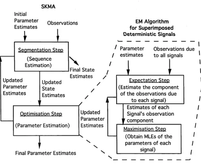
Figure 3.1: Joint State Sequence and Parameter Estimation using

the SKMA and EM algorithms... 37

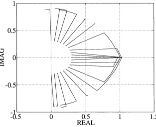
Figure 3.2: Estimation trajectory for initial phase estimates

between ±7t/2 - p0 = 2.5... 39

Figure 3.3: Estimation trajectory for initial phase estimates

between ±rt/2 - p0 = 0.3...40

Figure 3.4: Estimation trajectories for 30 realisations - p0 = 2.5 & \j/0 = 0.4... 40

Figure 3.5: Performance of the VA verse AOA - 20dB/Sensor Signal... 42

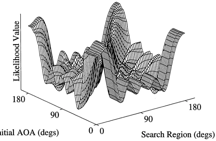
Figure 3.6: Likelihood function surface, Initial AOA estimate vs Search Region,

First Iteration - 20dB/Sensor signal...43

Final Iteration - 20dB/Sensor signal...43

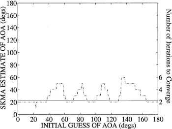
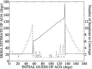
Figure 3.8: Final AOA estimate vs Initial Guess AOA (solid line) with Number

of Iterations of the SKMA to converge (dashed line) - 20dB/Sensor

(15)

,44 Figure 3.9: Performance of the VA verse AOA - OdB/Sensor signal...

First Iteration - OdB/Sensor signal... 45

Figure 3.11: Likelihood function surface, Initial AOA estimate vs Search Region, Final Iteration - OdB/Sensor signal... 45

Figure 3.12: Final AOA estimate vs Initial Guess AOA (solid line) with Number of Iterations of the SKMA to converge (dashed line) - OdB/Sensor signal...46

Figure 3.13: AOA estimation for one signal ML vs SKMA methods... 47

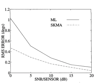
Figure 3.14: AOA estimate variance for one signal ML vs SKMA methods...48

Figure 3.15: BER for one signal ML vs SKMA methods...48

Figure 3.16: RMS Error for CC signal vs tone using the SKMA method...50

Figure 3.17: RMS Error for CC signal vs Broken signal using the SKMA method...50

Figure 3.18: AOA estimation for two signals ML vs SKMA vs SKMA-EM methods...53

Figure 3.19: Probability of resolution for two signals: ML vs SKMA vs SKMA - EM methods...53

Figure 3.20: Average BER for two signals ML vs SKMA vs SKMA-EM methods...54

(16)

Figure 3.22: Probability of resolution for two signals, when estimating two signals

but one is broken - ML vs SKMA - EM methods... 56

Figure 3.23: BER for one signal, when estimating two signals but one is broken -ML vs SKMA - EM methods...57

Figure 4.1: Ave. BER for VA, RCVA and RSSE (|a = 2) with no parameter estimation... 73

Figure 4.2: Ave. BER and AOA estimates using RSSE (p. = 2)... 77

Figure 4.3: Ave. BER and AOA estimates using RCVA (p = 2)... 77

Figure 4.4: Ave. BER and AOA estimates using an on-line VA... 78

Figure 5.1: Four-State Trellis, 5 time units with branch lengths labelled...85

Figure 5.2: State sequence estimate obtained via the VA... 85

(17)

Abbreviations

A M P P A P o ste rio ri M a x im u m P a th P ro b ab ility . A O A A n g le O f A rriv al.

A R A u to -R e g re ssiv e . B E R B it E rro r R ate.

C C C o n v o lu tio n a l C o ded.

C D M A C o d e D iv isio n M u ltip le A ccess.

dB d e c iB e l.

D F D irectio n F in d in g .

D S P D ig ital Signal P ro c e ssin g . E M E x p e c ta tio n M a x im isa tio n . E q n E q u a tio n n u m b e r.

E -step E x p e c ta tio n step .

F D M A F re q u e n c y D iv isio n M u ltip le A ccess. F I M F is h e r In fo rm a tio n M atrix .

G F G a lo is F ield.

G S M G lo b a l S y ste m fo r M o b ile co m m u n ica tio n s. H F B A H M M F o rw a rd B a c k w a rd A lg o rith m . H M M H id d e n M a rk o v M o d el.

IC A S S P In te rn a tio n a l C o n fe re n c e on A co u stics, S peech and S ig n al P ro cessin g .

I E E E In stitu tio n o f E le c tric a l and E le c tro n ic E n g in eers.

(18)

LSB Least Significant Bit.

MA Multiple Access.

MAP Maximum A Posteriori Probability.

ML Maximum Likelihood.

MSB Most Significant Bit.

M-step Maximisation step.

MUSIC Multiple Signal Classification.

NCDMC Nearly Completely Decomposable Markov Chain.

PDMA Polarisation Division Multiple Access.

QPSK Quadrature Phase Shift Keyed.

RCVA Reduced Complexity Viterbi Algorithm.

RMS Root Mean Square.

RSSE Reduced State Sequence Estimation.

SDMA Space Division Multiple Access.

SKMA Segmental K-Means Algorithm.

SNR Signal to Noise Ration.

TDMA Time Division Multiple Access.

ULA Uniform Linear Array.

VA Viterbi Algorithm.

VFBA Viterbi Forward Backward Algorithm.

(19)

Glossary

A T ra n s itio n p ro b a b ility m a trix . 8 (0 ith g e n e ra tin g p o ly n o m ia l.

A(n(t)) A rra y ste e rin g m a trix . _gj° j th c o e ff ic ie n t o f ith g e n e ra tin g

a ij T ra n s itio n p ro b a b ility , sta te i p o ly n o m ia l.

t o j . H N o . o f in te rv a ls in a s e a rc h

B O b s e rv a tio n sy m b o l g rid .

p ro b a b ility m atrix . h D e la y a fte r w h ic h a sta te

B H a n k e l M a trix o f m e s s a g e b its. d o e s n ’t a ffe c t an o b s e rv a tio n .

* i(U (t)) P ro b a b ility o f o b s e rv in g sta te j

g iv e n o b s e rv a tio n U (t).

I<(0 D e fin e d u s in g th e F IM o r s c o re

v e c to r o f Q , ( t ) .

b (t) M e ss a g e b its. I Id e n tity M a trix .

C (q t) M o d u la tio n fu n c tio n . i In d e x c o u n te r.

c (k ) B its o f C o n v o lu tio n a l C o d e ’s _j In d e x c o u n te r.

sh ift re g iste r. K N o . o f s e n s o rs in U L A , a lso

d U L A s e n s o r s p a c in g . S lid in g w in d o w siz e .

d (k ) B its o f C o n v o lu tio n a l C o d e ’s k In d e x c o u n te r - n o. o f se n so rs .

s h ift re g is te r. L (0) L o g - lik e lih o o d fu n c tio n .

djOi) C o n tin u o u s fu n c tio n m a p p in g L N o . o f s ig n a ls .

9 T to 9 T . i In d e x c o u n te r - n o . o f sig n a ls. F N o . o f sta te s. M N o . o f p h a s e s ig n a llin g v a lu e s .

G T o e p litz M a trix o f g e n e ra tin g N (t) A d d itiv e W G N m a trix .

p o ly n o m ia l(s ). N C o n s tra in t L e n g th .

(20)

p(n) O rth o g o n a l p ro je c tio n m a trix _{u f} E n c o d e d b its d u e to ith

s p a n n in g c o lu m n s o f A ( 0 ( t ) ) . _{g e n e ra tin g p o ly n o m ia l.}

p (t), P (t) P a rtitio n o f s(t), S (t). v(t) A d d itiv e W G N .

Q N o. o f g e n e ra tin g p o ly n o m ia ls . w f T o e p litz m a trix o f le ft n u

ll-QXO L o g -lik e lih o o d fu n c tio n . v e c to r w f .

qt S ta te at tim e t. W j , w M a tric e s o f W f . 9 T A ll n o n -n e g a tiv e re a ls W j , w f L e ft n u ll-v e c to r(s ).

n u m b e rs. w (i)w jk k th c o e ffic ie n t o f w f .

R S a m p le c o v a ria n c e m atrix . w (t), w t A d d itiv e W G N .

R ( 0 N o ise c o v a ria n c e m atrix . x(t) R e a l c o m p o n e n t o f tra n s m itte d

r(t), R (t) P a rtitio n o f s(t), S (t). sig n a l.

s(t), S (t), y (t) Q u a d ra tu re c o m p o n e n t o f

Si S ta te o f C o n v o lu tio n a l C o d e (s) tra n s m itte d s ig n a l.

sh ift re g iste r. z M e ss a g e b its c o d e d at o n e

T B lo c k le n g th o f d ata. tim e.

t In d e x c o u n te r - tim e. z(s(t), 0 ( t ) ) ,

U H a n k e l m a trix o f e n c o d e d b its. z (t), Z (t) C o m p le x tra n s m itte d s ig n a l(s ). u (t), U (t), z j D e la y o p e ra to r.

u t O b s e rv a tio n (s ).

a t(0 H M M ’s fo rw a rd in fo rm a tio n _{Y ((t)} R e p re s e n ts e a c h p a ra m e te r o f

p ro b a b ility m e a su re . th e £ th sig n a l.

P,(i) H M M ’s b a c k w a rd in fo rm a tio n _{Y ,(0} T h e H M M ’s a p o s te r io r i

p ro b a b ility m e a s u re . in fo rm a tio n p ro b a b ility

ß ,( i) V F B A ’s b a c k w a rd p a th m e a s u re fo r th e ith sta te .

in fo rm a tio n p ro b a b ility Y ,0 ) T h e V F B A ’s A M P P m e a s u re

(21)

5,(0 V A and V F B A ’ s forw ard path % Convergence criterion

inform ation probability threshold.

measure. K In itia l state distribution

c« A rb itra ry real-valued scalars, probability vector.

that sum to 1. n Pi (= 2%).

0 , 0 ( t) Parameter vector. 7 t i , 7E(i) P robability o f in itia lly being

e, e(t) A O A ’ s azimuth o f signal. in state i.

er(i) H yb rid algorithm ’ s a _P _{A m plitude vector o f signals}

p o s te r io r i inform ation _p.pW A m plitude o f signal.

probability measure. a Noise standard deviation.

< ( i ) H yb rid algorithm ’ s forward a 2 Noise variance.

inform ation probability H yb rid algorithm ’ s backward

measure. inform ation probability

X H M M parameter set. measure.

X Signal wavelength. cp, cp(t) A O A ’ s elevation o f signal.

n Reduced memory o f Phase offset vector o f signals.

Convolutional Code, also a \|/, \|/(t) Phase offset o f signal. positive real parameter used in V ,( i) M a trix fo r V A backtracking.

(22)

Chapter 1 Introduction

A he estimation of superimposed signals occurs in a variety of electromagnetic

radiation systems, including: communications, medical imaging and radar. The

detection and estimation of superimposed signals was studied by Wax in 1985. His

dissertation “addresses the problem of estimating the number, the parameters and the

waveforms of superimposed signals, occurring in a variety of fields ranging from

radar, sonar, oceanography and seismology to medical imaging and radio-astronomy”

[Wax 1985].

Wax traced the history of the superimposed signals problem from its possible

beginnings in 1795, when Gaspard Riche, Baron de Prony published his work on

fitting superimposed exponentials to data.

This dissertation examines the problem of digital communication signals, in

particular, convolutional coded signals (described in Section 1.2). The transmission

of digital data has become prolific in the last decade or so, and continues to grow

rapidly as digital signal processing (DSP) chips become smaller, faster and more

affordable. Convolutional codes are very popular in digital communications systems

(e.g. satellite communications [Intelsat 1987] and more recently digital mobile

cellular phone [Padgett et al. 1995, Steele 1992] systems) because of their optimal

decodability by the efficient Viterbi algorithm (VA) [Viterbi 1967, Forney 1973]. A

(23)

Communications systems use Multiple Access (MA) schemes to allow multiple

signals to be received apparently simultaneously. These MA schemes include: Time

Division MA (TDMA); Frequency Division MA (FDMA); Code Division MA

(CDMA); Space Division MA (SDMA); and Polarisation Division MA (PDMA).

However, only one signal can be received in each division at any one time, i.e. in each

time division for TDMA, in each frequency division for FDMA, using each (nearly)

orthogonal code for CDMA, by directing spot beam antennas at each signal for

SDMA, and in each polarisation for PDMA. Using an array of sensors, a method is

developed which can accurately demodulate superimposed convolutional coded

signals and thus could be used to increase the throughput of digital communications

systems which use these MA schemes. Array processing techniques have been used

to spatially filter superimposed signals before individually demodulating them

[Haykin 1991]. Currently, spatial filtering of signals requires the estimation of each

signal’s angle of arrival (AOA) using direction finding (DF) techniques [Hurt 1990].

These techniques use no knowledge of the models of the signals being received. The

method developed in this dissertation improves the accuracy (when compared to

deterministic maximum likelihood (ML) methods, e.g. the method by Wax [1985],

which is briefly described in Appendix E) of estimating superimposed signals, by

using knowledge of the signal models. The method jointly estimates each signal’s

parameters (e.g. AOA) and demodulates them. Suboptimal methods which reduce the

computational complexity of the above joint estimation technique are also developed.

These include: the use of the expectation maximisation (EM) algorithm for

superimposed deterministic signals (which is briefly described in Appendix D); the

development of a reduced complexity Viterbi algorithm (RCVA); and the

development of a reduced complexity on-line joint estimator using both the RCVA

and EM algorithms in on-line modes.

In order to decode a convolutional coded signal the VA requires exact knowledge of

(24)

convolutional encoder’s structure from the received signal is developed in this

dissertation.

The VA maximises a forward path probability (see Appendix A) in order to estimate a

ML state sequence, via a backtracking procedure, from noisy observations. In an

analogous manner a backward path probability is generated, replacing of the

backtracking procedure. This lead to the development of a Viterbi forward-backward

algorithm (VFBA). This algorithm computes an a posteriori maximum path

probability (AMPP) for each state at each time thereby providing a confidence level

for each state estimate. The similarity of the VFBA’s structure with that of the hidden

Markov models (HMMs) forward-backward algorithm (HFBA), which is used for

Maximum a posteriori Probability (MAP) state estimation, is exploited to develop a

hybrid algorithm. A description of the hidden Markov model is given in Section 1.3

and the HFBA in Appendix B. The hybrid algorithm provides a method to adaptively

interpolate between obtaining the ML path estimate and MAP state estimate from

noisy observations of a Markovian state sequence.

The rest of this chapter provides brief introductions on a number of topics which

provide background information to this dissertation. The topics are: a

communications system; convolutional coded signals; the hidden Markov model

(HMM); and array processing. Known algorithms which are used in this dissertation

are briefly described in Appendices A - E with references to material which can

provide the reader with more detailed explanations. The algorithms are respectively:

the Viterbi algorithm (VA); the HMM forward-backward algorithm (HFBA); the

segmental k-means algorithm (SKMA); the expectation maximisation (EM)

algorithm for superimposed deterministic signals; and direction finding via a method

of maximum likelihood.

At the end of this chapter the algorithms developed in this thesis are summarised and

(25)

§1.1 Communications System

A communication system’s function is to transmit information from a source to a

destination via a channel using some carrier signal. The basic communication system

consists of the following components.

Source —> Transmitter —> Channel —> Receiver —> Destination.

In this dissertation only a digital system is considered. In a basic digital system, on

the source side the information is formatted and modulated before being transmitted

into the channel, however in more complicated systems it may also contain encoding

(source and channel), encryption, multiplexing, frequency spreading and multiple

access components. At the receiver there needs to be the corresponding inverse

components in order to recover the original message. The reader is referred to any

digital communications text book for more information, e.g. Sklar [1988] or Haykin

[1988].

The only extra component added to the basic digital system, described above, (that is

considered in this dissertation) is that the information bits are convolutionally

encoded prior to transmission. It is assumed that: the channel only adds white

Gaussian noise (WGN) to the signal(s); does not impose any inter symbol

interference (ISI) on the signal(s); is void of multipath; the receiver samples the

signal(s) once per baud; when multiple signals are being sampled, the signals have

the same baud rate; and the signal(s) have been mixed down to baseband.

The ISI and equalisation problems in the reception of digital communications signals

are not considered in this dissertation as they are outside the scope of this work.

Eyuboglu and Qureshi [1988], Duel-Hallen and Heegard [1989], Hagenhauer and

Hoeher [1989], Tong et al. [1991 and 1993], Moulines et al. [1994] and Xu et al.

(26)

§1.2 Convolutional Coded Signals

Convolutional codes were first proposed by Elias in 1955. A convolutional coded

signal has digital input information bits (the message sequence) b(t), t > 0 which can

be denoted as a first order Markov process. If the b(t)s are an independently and

identically distributed (i.i.d.) equiprobable binary process, then the transition

probabilities , = 0.5 for i,j =0,1. The message sequence can be convolutionally

encoded via a linear operation (over GF(2), i.e. modulo-2, [Blahut 1984]) using N-l

shift registers and Q generating polynomials to produce a constraint length N and rate

yQ

(where Q coded bits are produced for every Z information bits) convolutional coded bit stream. The coded bit stream is then transmitted using a modulation

scheme. If M-ary phase shift keyed modulation [Sklar 1988] is used, the coded bits

determine one of M = 2Q possible phase signalling values. The phase value, <J)(t), of

the signal is thus determined by:

where Gm(n) are known binary coefficients of the convolutional code’s generating

polynomials.

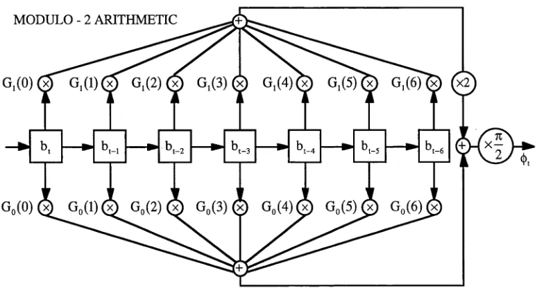
Figure 1.1 shows how to generate a rate

lA,

constraint length 7, convolutional coded quadrature (i.e. M = 4) phase shift keyed (QPSK) signal* * from the binary input

information bits, b(t) using the generating polynomials G0(n) and G,(n).

Combining convolutional coding and QPSK modulation as in Eqn. (1.1) is done so as

to reflect the way it is done in the possible application areas. Some satellite

communication systems (e.g. Intelsat [1987]) use punctured QPSK convolutional

coded signals. Punctured codes can be decoded as unpunctured codes with minimal

* ay is the transition probability from state i to state j.

* The theory presented in this thesis is not restricted to just QPSK signals, any digital modulation

type may be used.

M - l N —1

(27)

increase in complexity [Bibb Cain et al. 1979]. Digital mobile phones (e.g. GSM)

[Padgett et al. 1995, Steele 1992] use convolutional coded signals with QPSK

modulation or its variants [Falconer et al. 1995].

Figure 1.1: Generation of a Convolutional Coded QPSK Signal.

Let

s(t) = [b(t - N +1)... b(t - l),b(t)] (1.2)

be the state of the convolutional code’s shift register at time t. The state sequence

{s(t)j is a first order Markov process having F = 2N states with transition

probabilities:

Pr{s(t) = [c(N - l),...,c(0)] I s(t -1 ) = [d(N - l),...,d(0)]} =

j ad(o)c(o) < j) = d ( j- l) , 1 — j — N — 1

I 0 else

where the c(j)s and d(j)s are dummy

variables used to represent the elements

[image:27.515.41.428.131.347.2]

(28)

In this thesis attention is focused on the uniform i.i.d. message case, although such a

restriction is not necessary for any of the analysis presented herein to remain valid.

Each s(t) corresponds to a certain (j)(t), hence the transmitted signal is modelled by

z(s(t),0(t)) = p(t)el(4>(0+v,,(t)) = x(t) + i y(t) with x(t) = p(t) cos((})(t) + \|/(t))

y(t) = P(t) sin(<J>(t) + V(t)) (1.4)

where O(t) is a parameter vector of the signal’s

amplitude (p(t)) and phase offset (\|/(t)).

In 1967, Viterbi proposed an algorithm for decoding convolutional codes. The

algorithm uses forward dynamic programming and is a maximum likelihood decoder

[Omura 1969]. This algorithm later became known as the Viterbi Algorithm (VA),

and is briefly described in Appendix A.

Sklar [1988] lists the best known generating polynomials for convolutional codes

having rate y2, constraint lengths 3 to 9, and rate ]/3, constraint lengths 3 to 8, these

codes were determined by Odenwalder in 1970.

§1.3 The Hidden Markov Model

The basic filter theory for HMMs was first presented by Baum and his colleagues in a

series of papers in the late 1960s and early 1970s [Baum and Petrie 1966, Baum and

Egon 1967, Baum and Sell 1968, Baum et al. 1970, Baum 1972]. These papers

developed statistical estimation algorithms for discrete Markov processes'! observed

(hidden) in noise. The model structure became known as a hidden Markov model and

since the mid-1980s has become increasingly popular in engineering applications, due

in part to introduction and tutorial papers by Rabiner and Juang [1986] and Rabiner

[1989].

(29)

Consider the following system known as a HMM (cf. Rabiner [1989]). Assume a

finite number, F, of states, S = {S,,S2,...,SF}, and denote the state at time t by qt.

The process is assumed to be first order Markovian, that is:

Pr{q,+i = s j|q, = s i.q,-i = s k.---}

= Pr{qI+i = S j| q , = S i}:=aij

(1.5)

where aij5 1 < i, j < F is known as the state transition probability from state Sj to state

Sr

The states are observed via a process:

u . = c ( q ,) + w, (1.6)

where C( ) is a deterministic function (which in a communications system, would be

determined by the modulation type of the signal) and wt is the noise process. Denote

the probability density function of wt by /(•). The probability of observing Ut given

state Sj at time t, ^(U ,), is given by:

1 < j < F (1.7)

Typically we assume WGN with variance a 2, thus:

— 7 = exP

CW27T

1 < j < F (1.8)

Finally the model is completed with an initial state distribution vector n , where

(30)

In signal processing applications, when no a priori state information is known, n is

usually chosen uniform, i.e. n =

The HMM is defined by the parameter set:

X = (n,A,B\ (1.10)

where A and B are the matrices containing the ays and ^ (U t)s respectively.

In HMM processing, given an observation sequence and model, a goal may be to

estimate a state sequence which is optimal in some sense.

If the objective is to determine, at each separate time, the states which are individually

most likely, then the MAP (or minimum variance / conditional mean) state estimates

can be determined using the HFBA. The HFBA is briefly described in Appendix B.

If the objective is to determine the most likely state sequence, over all the data, then

the ML state sequence estimate can be determined using the VA. The VA is briefly

described in Appendix A.

Further details and tutorial introductions to HMMs are provided by Rabiner and Juang

[1986], Poritz [1988], and Rabiner [1989].

§1.4 Sensor Array Processing

In Chapters 3 and 4 the concern is with superimposed signals which are transmitted

on the same frequency, at the same time, and possibly with the same convolutional

encoding scheme, the signals however may be coming from different locations, and

with different input information bits. Figure 1.2 shows how an array of sensors may

(31)

In this dissertation the following assumptions are made about the array and signals.

The assumptions are: the sensor (antenna) patterns are known; the number of signals

incident on the array is known; and the sources are located in the far-field of the

array, permitting the narrowband approximation (i.e. planar wavefronts). These

assumptions are commonly made in array processing research [Hurt 1990, Haykin

1991] and are generally accepted as valid in most practical situations. This said,

research has previously been conducted into: array shape estimation; the reception of

wideband signals; and signals which are within finite range, see Haykin [1991] and

Hurt [1990] for more details on the research in these areas. Research has also been

conducted into determining the number of signals, e.g. Wax [1985] and Wu et al.

[1995].

Figure 1.2: Superimposed signals received via an array of sensors.

The signal model for this situation is: Consider L superimposed signals each

generated as described above by Eqns. (1.1) to (1.4), except that the input message

sequences, jb w(t)j, 1 <

t

< L, are generated independently and the generating polynomials G ^(n) for each signal may be different. These signals are incident on

an array of K sensors. The baseband model of the K-vector array outputs, U(t), is

given by:

(32)

for t = 0 , . . . , T - 1, and where A(Q(t)) is the so-called direction matrix [Haykin 1991] that depends on the arrival angles Q(t) = [cp(1)(t),0(1)(t),...,(p(1,(t),0(1'(t)] of the signals

Z(t) = [z(1)(t),z(2)(t),_,z(L)(t)]T (where q><0( t ) , 0(/)(t) refer to the elevation and azimuth of signal z(/)(t) respectively), together with the array geometry. N(t) is a white Gaussian noise (WGN) process with covariance matrix R(t ) . The noise is stationary, independent, spatially white and of equal power from sensor to sensor (i.e.

R( t) = G2I ) .

The processing of superimposed signals generally involves the use of an array of sensors and beamforming techniques. These techniques sequentially estimate the signals parameters and then individually demodulate each signal. The signal models are only introduced in the final demodulation stage. Figure 1.3 shows this sequential procedure.

Demodulated

Signals

Demodulator

Receiver

_Estimator

AOA

_{of Baseband signals}

Estimation

Figure 1.3: Sequential scheme for estimation of superimposed signals.

(33)

Iterative techniques, such as the expectation maximisation (EM) algorithm [Dempster

et al. 1977] have also been applied to the problem of DF. For example, Feder and

Weinstein [1988] introduced the use of the EM algorithm for DF. Miller and

Fuhrmann [1990] derived EM algorithms for the ML estimation of the AOAs of

multiple narrow-band signals in noise, under both the deterministic and stochastic

signal models. Ziskind and Hertz [1993] derived an EM algorithm for Auto-

Regressive (AR) processes. Malcolm and White extend Ziskind and Hertz’s EM

algorithm for general linear Gauss-Markov processes by refining the E-step.

Knowledge of the signals characteristics has also been used to improve the AOA

estimates, e.g. Trudinger and White [1994] and Talwar et al. [1994]. Li and Compton

[1993] incorporate knowledge of one or all of the signals waveforms to improve the

accuracy of the AOA estimates and Agee et al. [1990] use knowledge of the signals’

cyclic frequency in order to achieve blind adaptive signal extraction.

In Chapter 3, the sequential method shown in Figure 1.3 is used for performance

comparison. The AOA estimates, i.e. QML, are obtained via the method of ML due to

Wax [1985], which is briefly described in Appendix E, and the estimates of the

baseband signals, i.e. ZML(t), are obtained as follows:

ZML(t) = A ^(Ö ML)AH(Ö ML)u (t) (1.12)

where A +|o mi J is the pseudo inverse of Ah|q mi Ja|Omi J and is determined via a

singular value decomposition, this is in case ^Ah(O m1 )a^Qmi JJ does not exist.

State estimates for each signal, i.e. s{0(t), are then obtained by applying the VA to

each ML baseband signal estimate, i.e. z(Mj (t), individually. This sequential ML

(34)

§1.5 Thesis Contributions

The contributions of this thesis and the algorithms (methods) developed are now

listed.

• Estimation of the Structure of a Convolutional Coded Signal: A technique for determining the constraint length and generating polynomials

(structure) of a rate / Q convolutional coded signal from only the received

signal is developed.

• The use of State Sequence Estimation combined jointly with Parameter Estimation in Array Processing problems: A method for jointly demodulating superimposed convolutional coded signals and estimating their

parameters using knowledge of the models (and structure) of the signals is

developed. A modification incorporating the EM algorithm in the parameter

estimation step is also developed to reduce some of the computational

complexity.

• A Reduced Complexity Viterbi Algorithm: Standard reduced state sequence estimators (RSSE), developed for ISI problems, maintain a fixed

number of reduced states, however when there are only a few observations

and many states (as in the superimposed convolutional coded signals

problem), the RSSE techniques may have trouble acquiring lock onto the

correct state sequence. The RCVA differs from standard RSSE algorithms in

that the number of reduced states is adaptively varied. This modification

improves (on average) the probability of acquiring (and maintaining) lock

onto the correct state sequence when estimating superimposed convolutional

coded signals.

(35)

developed. This estimator reduces the computational complexity of the

above joint estimator by using the RCVA and EM algorithms in on-line

modes. It also enables signals with varying AOAs to be successfully

tracked.

• A Viterbi Forward-Backward Algorithm: The forward backward algorithm is derived from the VA. By presenting the VA’s path metric as a

forward path probability, a backward path probability is derived in an

analogous manner. Combining these two probabilities gives a Viterbi

forward-backward algorithm. The VFBA computes an a posteriori

maximum path probability (AMPP) for each state, at each time, maximised

over all state sequences passing through that state, thus yielding uncertainty

information about each state estimate, this information is not available

directly from the VA. The estimated state sequence obtained via the VFBA

is the same as would be obtained via the VA.

• A Hybrid Viterbi / HMM Forward-Backward Algorithm: The VFBA above is closely related to the HFBA. This lead to the development of a

hybrid algorithm which interpolates between estimating the ML path

sequence (via the VA) and estimating MAP state estimates (via the HFBA).

The algorithm provides a method for adaptively varying the degree of

reliance on path constraints in obtaining state sequence estimates.

§1.6 Thesis Structure

The structure of the thesis is now outlined.

In Chapter 2 a technique for determining the structure (constraint length and

generating polynomials) of a convolutional coded signal, from only the received

encoded binary data is developed. This technique is confined to the special case of

(36)

equalisation of digital communication channels [Moulines et al. 1994, Tong et al.

1991 and 1993, Xu et al 1994].

In Chapter 3 a method for jointly demodulating and estimating the parameters of

superimposed convolutional coded communication signals incident on an antenna

array is developed. The method is based on the segmental k-means algorithm

(SKMA), a HMM based technique. A brief description of the SKMA is given in

Appendix C. The SKMA is an iterative procedure with two steps per iteration. This

allows the joint estimation in which the signals are estimated (demodulated), given

parameter estimates and the parameter estimates are updated given the demodulated

signals. A modification of the parameter estimation step is introduced in order to

reduce its computational complexity. The modification applies the EM algorithm for

superimposed deterministic signals. Both estimators are then compared to the

deterministic ML estimation method described in Section 1.4.

In Chapter 4 a reduced complexity on-line estimator is developed for the problem of

jointly demodulating and estimating the parameters of superimposed convolutional

coded signals incident on an antenna array. A RCVA is first developed to reduce the

computational complexity of jointly demodulating multiple convolutional coded

signals via the VA. The RCVA is a modification of the RSSE algorithms developed

for ISI problems. The RSSE maintain a fixed number of reduced states, whereas the

RCVA adaptively varies the number of reduced states in order to acquire and maintain

lock onto the correct state sequences. The on-line estimator jointly uses the RCVA

and the EM algorithms in on-line modes. Simulations are used to demonstrate the

algorithm and provide comparisons of the computational complexities of the various

methods discussed.

In chapter 5 a connection between ML path estimation from noisy observations of a

Markovian state sequence and MAP state estimation is developed. The classical VA

(37)

a backward path probability is generated which lead to the development of a VFBA.

The VFBA computes an a posteriori maximum path probability for each state at each

time, thus providing a confidence level for each estimated state. Confidence levels

are not available from the VA, due to the hard decision backtracking process. The

similarity of the VFBA’s structure with that of the classical HFBA (used for MAP

state estimation) is exploited to obtain a hybrid Viterbi / HMM forward-backward

algorithm.

In Chapter 6 a summary of the thesis and conclusions are presented. Suggestions for

areas in which further investigation may be conducted and ideas for future research

(38)

Chapter 2 Estimating the Structure of a

Convolutional Coded Signal

§2.1 Introduction

Convolutional codes (originally proposed by Elias in 1955) are very popular in

digital communications (e.g. satellite systems [Heller and Jacobs 1971, Intelsat 1987]

and digital mobile phone systems, such as the GSM system [Steele 1992]). This is

because convolutional codes provide forward error correction and are optimally

decoded by the efficient Viterbi Algorithm [Viterbi 1967]. The VA, like all trellis

search algorithms, presumes exact knowledge of the structure of the convolutional

encoder (i.e. its constraint length and generating polynomials). In some applications

this knowledge may not be available and hence must be extracted from the received

signal.

In this chapter a technique is developed for determining the constraint length and the

generating polynomials from encoded binary data. The technique is confined to the

special case of rate / Q convolutional codes and is based on a novel approach recently

introduced for blind equalisation of digital communication channels [Moulines et al.

1994, Tong et al. 1991 and 1993, Xu et al. 1994],

In Section 2.2 the problem is formulated, Section 2.3 describes the key properties

(39)

structure of the convolutional coded signal and conclusions are presented in

Section 2.5.

§2.2 Problem Formulation

Consider a rate / Q, Q > 2, convolutional encoder with constraint length N, and generating polynomials g(,) = [ g ^ g ^ ,,...,^ 0] , g-0 e{0,l} , 1 < i < Q.

Let {bt} , bt e {0,1}, denote the input bits to the convolutional encoder. The encoded

bits due to the ith generating polynomial are determined by:

“ ?, = X g i V J+. i = 1 , , Q (2.1)

j=l

where the arithmetic is over GF(2), i.e. modulo-2, [Blahut 1984].

The fundamental problem can be now stated as follows. Given T samples of encoded

bits {u«} 1 < i < Q, determine the constraint length N and the generating

polynomials g(l).

To solve the problem we make the following assumptions:

N - l

Al: The generating polynomials g(l)(z) = ^ g j ,)z_j have no common factors. j=0

A2: The constraint length N satisfies N < K, with K some known number.

A3: The input bits {bt} are i.i.d. random variables.

A l implies that the convolutional code is non-catastrophic, which is generally the case

in practice. A2 implies that the upper limit on the constraint length is known. A3 is

(40)

§2.3 The Key Properties

Using a sliding window of length K, Eqn. (2.1) can be rewritten in the following

matrix form (where ® stands for matrix multiplication with the arithmetic over

GF(2)):

1

•• u(i) _{U T - K +}₁1 _{g N} _{g N - ,} _{g l ’’} 0 '

U (i)

u 2 » ?> •.. u(i)u T - K+2 ₌ g N g (N - l g ! 1’

U (i)

L K u L • 0 g (N -l gS, } .

b.

b2

b 2

b 3

b T - ( N + K -2) b T - ( N + K -3)

(2.2)

b_{N + K - l} _{'N + K}_{- 2} b T

Denoting by G(l) the Kx(N+K-l) Toeplitz matrix of the ith generating polynomial as:

G(i) =

s (i)

ON g (N - l g ! ° 0 0

0 _{g N} _{g N - .} _{g (i °} 0

0

0 0 _{g ?} _{g (N}_-1 _• _{g ! °}

(2.3)

and by U(l) and B the Kx(T-K+l) and (N+K-l)x(T-K+l) Hankel matrices as:

U(i) =

» ? > U ? • •• u (i)U T - K + 1

U?

u « . •• u (i)_{u T - K}₊₂

< U « , ■"

u?

(2.4)

(41)

t) _b _{• •} _b

u 2 u T - ( N + K - 2 ) b 2 b 3 b T - ( N + K - 3 )

N + K - l b N + K - 2 bT

(2.5)

Eqn. (2.2) can be rewritten as:

U(i) = G(i) <8>B i = 1 , , Q (2.6)

Concatenating the matrices U(,), i = 1 ,... , Q, gives:

U = G ® B

where U is the KQx(T-N+l) matrix:

U =

u(1)

u(Q)

(2.7)

(2.8)

and G is the KQx(N+K-l) matrix:

G = 'G(1)'

g(q)

(2.9)

The two key properties upon which the solution is based are now stated.

Theorem 2.1: Under assumptions A1 and A2, the matrix G is full column rank.

(42)

Theorem 2.2: Under assumptions A l - A3, the rank of U is:

RankGF(2) U = N+K-l (2.10)

with probability which approaches one as T —» °o.

Proof: From Theorem 2.1:

RankGF(2)G = N+K-l (2.11)

Now from A3 it follows that if T —» °° the matrix B is full-row rank with probability one, i.e.

RankGF(2)B = N+K-l (2.12)

The result now follows readily by using (2.11) and (2.12) in (2.7).

Note that for Theorem 2.2 to hold with probability close to one it suffices that the

number of columns in B is much larger than the number of rows, that is T-K+l »

N+K-l, which implies T » 3K+1. □

Theorem 2.3: Under assumptions A l - A2, the left null-space of G determines the generating polynomials coefficients |g (l)

j

up to a multiplicative constant.

Proof: See Moulines et al. [1994]. □

§2.4 The Solution

The constraint length N is readily determined from the rank of U.

(43)

j = 1 ,...,K Q -(N + K -1 ) (2.13)

Wj ® U = 0

From Eqn. (2.7):

Wj ® G ® B = 0

which implies, since B is full-row rank, that:

Wj ® G = 0

Let , 1< i < Q, be the ith lxK block of w ., i.e.

w j= ... W «>

where

]

Now (as can be readily verified) the following structural relation holds,

Wj ® G = g ® Wj j = 1 KQ-(N+K-1)

where

with

(2.14)

(2.15)

(2.16)

(2.17)

(2.18)

(2.19)

(44)

and

W =

W,(Q)

(2.21)

w ith Wj(l) being the N x (N + K -l) Toeplitz matrix:

(2.22)

From Eqns. (2.15) and (2.18),

g (8)Wj = 0 j = l ,...,K Q - ( N + K - 1 ) (2.23)

w hich can be rew ritten as

g ® W = 0 (2.24)

where

w = [w, ,w2, . . . ,wkq_(N+k_1)] (2.25)

(45)

The solution can be summarised as follows:

(1) Determine the rank of U.

(2) Determine N using Eqn. (2.10).

(3) Compute a left null-vectors w j of U, j = 1 ,..., KQ - (N+K-l). (4) Using Wj construct W ^, i = 1 ,..., Q using Eqn. (2.22).

(5) Construct W| using Eqn. (2.21). (6) Construct W using Eqn. (2.25).

(7) Compute g (and hence the g(l) s) as the left null-vector of W.

Notice that steps (1), (3) and (7) are over GF(2).

§2.5 Conclusion

The method described in this chapter does not require the received encoded data to be

noiseless, rather it requires that hard decisions on a set of T consecutive samples of

the noisy data be error-free. If any errors occur in the set of T consecutive samples

(46)

Chapter 3 Joint Demodulation and Parameter

Estimation

§3.1 Introduction

The problem addressed in this chapter and in Chapter 4 is the spatial filtering of

superimposed convolutional coded QPSK communications signals incident on a

Uniform Linear Array (ULA) of sensors. A method for jointly demodulating the

signals and estimating the signals’ parameters, e.g. amplitude, phase offset and angle

of arrival (AOA), is developed.

The estimation of superimposed signals incident on an array of sensors is not new, see

Chapter 1, Section 1.4 for details. This chapter investigates the estimation of

superimposed signals modelled as Markovian sequences. These Markovian

sequences (convolutional coded signals) have strongly constrained path sequences

and therefore the estimation procedure should yield valid path constrained sequences

[Sklar 1988]. Knowledge of the signals’ models is assumed (i.e. each signal is

convolutional coded with known constraint length and generating polynomials).

The segmental k-means algorithm (SKMA), a HMM based technique, is applied to

the problem (see Appendix C for a brief description of the SKMA). This algorithm is

an iterative procedure requiring two steps per iteration. The first step (segmentation

(47)

signals) given estimates of the signals’ parameters, this is accomplished using

dynamic programming via the VA. The second step (optimisation step) uses the

estimated ML state sequences to refine estimates of the signals’ parameters by

maximising the state-optimised log likelihood function with respect to the parameters.

A modification of the method which decreases the computational complexity of this

problem and hence the processing time is also described. The modification makes use

of the EM algorithm for superimposed deterministic signals (briefly described in

Appendix D) in the optimisation step of the SKMA.

The methods developed are shown to improve the demodulation of the signals and in

addition improves the accuracy in estimating the AOAs, when compared to the

deterministic ML estimation method outlined in Chapter 1, Section 1.4. Superior

resolution capability for signals that are closely spaced is also demonstrated. The

improvements are shown to be significant for the examples discussed but are achieved

through an increase in the computational complexity of the problem. Monte Carlo

simulations are used to demonstrate the results and improvements obtained.

This chapter is organised as follows: In Section 3.2 a single signal (not incident on an

array) is used to provide a simple example for explaining and testing the SKMA. The

algorithm is used to jointly demodulate the signal and estimate the signal’s amplitude

and phase offset. In Section 3.3, the SKMA is described for a single signal incident

on an array (Section 3.3.1) and for superimposed signals incident on an array (Section

3.3.2). The expressions for demodulating the signal(s) and estimating the signal(s)’s

parameters are derived. The EM modification to the optimisation (parameter

estimation) step is also described in Section 3.3.2. Simulation studies are presented in

(48)

§3.2 Single Signal

The observed signal model for a single convolutional coded QPSK signal (defined in

Chapter 1, Section 1.2) is given by:

z(s(t),0(t)) = x(t) + i y(t) with x(t) = p(t) cos((j)(t) + \|/(t)) + w(t)

y(t) = P(t) sin(<t>(t) + \j/(t)) + v(t) (3 j )

where w(t), v(t) are i.i.d. WGN processes with zero mean and variance a 2.

The problem of interest is to jointly estimate the parameters ( p(t) and \j/(t) which can

be slowly varying with respect to time, but are considered constant for some block

length T+) and the message sequence jb(t)j (see Chapter 1, Eqn. 1.2) from the

The SKMA is a parameter estimation algorithm which involves data sequence

modelling. This algorithm was examined as a means of jointly demodulating the

signal and estimating the signal’s parameters. Juang and Rabiner [1990] provide

sufficient conditions for global convergence of the SKMA, however these conditions

are difficult to test and impose on the problems considered in this thesis. A local

convergence property for the algorithm applied to the problems in this thesis was

conjectured from the empirical evidence obtained, however a localised stability

analysis is intractable.

In the segmentation step of the algorithm, the objective (in a fixed interval

demodulation problem) is to estimate the ith iterative ML state sequence {ss (t)}:

{Sj (t)} = si (0)... si( T - l ) = arg max. Pr{s(0)... s(T - 1)| z(0),.... z(T - l);pi .xjr,}

(3.2)

(49)

for some signal block length T and ith estimates p, and tjr. It has been shown that

this problem can be solved using dynamic programming, resulting in the VA. The

VA is used in the segmentation step of the SKMA in preference to alternative

estimation algorithms (Bahl et al. [1974] and Baum et al. [1970]) for similar reasons

as those stated in Juang and Rabiner [1990], i.e. the requirement to reduce the

computational complexity, etc., of the problem.

The ith estimated ML sequence s; (t) = [ci(t — N +1),...,ci (t — 1), c{ (t)], 0 < t < T , where c^m) = 0, m < 0, is used to obtain an estimate of the message sequence |b i(t)|. If

the demodulated message bit (b i(t)) is obtained from the MSB o f Sj(t + N -1 ),

instead of the LSB of s4 (t), a smoothed sequence can be obtained as shown below:

The demodulated message sequence obtained from Eqn. (3.3) may be improved if

more accurate estimates of the signal’s amplitude and phase offset can be obtained.

The optimisation step of the algorithm uses the ith estimated ML state sequence

{sj(t)} and observation sequence {z(t)} to generate the next parameter estimates

( pj+,,\j/i+I). These estimates maximise the state-optimised log likelihood function: bi(t) = ci(t + N - l ) , 0 < t < T - N. (3.3)

(pi+, > V i.,) = arg maxjlog Pr{ {z(t)}| {s, (t)};p,\|/} }. (3.4)

(50)

2k m_1 n

where ^ ( t ) = — ^ 2 ' ”^ b i(t - n)G m(n), and

m=0 n=0

b ^ t) is obtained from Sj ( t) .

The updated estimates of the signal’s parameters are determined from Eqn. (3.5) using basic calculus and are given in closed form by:

P,+ l= ^ [ ( Y „ + X re)2 + ( Y re- X im)2]

f

\j/i+1 = arctan Y - X :

vYim + Xrey

where Y re = £ y ( t ) c o s ( ^ ( t ) ) , Y to = ^ y ( t ) s i n ( ^ ( t ) ) , (3'6)

t= 0 t= 0

X re = X x (t)c o s ($ ,(t)), X im = X x ( t) s in ( ^ ( t) ) .

t = 0 t= 0

These updated estimates ( p j+1 and \j/i+1) are used in the next segmentation step. The process is repeated until an imposed convergence criterion is satisfied, for example when the difference of two consecutive estimates of both p and \j) are smaller than or equal to given thresholds (£ ), i.e.

|pi+i - P i|^ %Pand |\jri+1 - \fr.| < (3.7)

§3.3 Array Processing

§3.3.1 Single Signal

(51)

The problem of interest here is to jointly estimate the amplitude (p), phase offset (\\f),

arrival angles ((p,0)* and the message sequence {b(t)} from the observed data

sequence {U(t)}.

Again, the SKMA method is used for demodulating the signal and estimating the

amplitude, phase offset and AOA of the signal. The approach is similar to the method

described above in Section 3.2 with minor changes to Eqn. (3.2) and Eqns. (3.4) to

(3.6). These new equations are as follows:

The ith estimated ML state sequence given in Eqn. (3.2) is now estimated by

determining:

{s,(t)} = 5,(0)... s,(T -1 ) = arg max Pr{s(0),.... s(T - 1)|U(0),.... U(T - l);p„ y, ,0,1

s(0),...,s(T-l) L J

(3.8)

for some block length T and ith estimates of pi5 xjq and Q;. The VA provides a

solution to the problem.

An improved estimate of the ML state sequence can be obtained if more accurate

estimates of the signal’s amplitude, phase offset and AOA are obtained. Thus, as in

Section 3.2, the state-optimised log likelihood function is used and Eqn. (3.4) is

rewritten as:

A + i ) = argmaxjlog Prj {U(t)}|{s,(t)};p,\|/,flJ). (3.9)

The output vector of the array, U(t), is written in quadrature baseband form as

u(t,k) = x(t,k) + i y(t,k) for each sensor, k. For a convolutional coded QPSK plane

wave signal, Eqn. (3.9) is rewritten as follows (using the azimuth angle 0t):

$ Again these parameters are assumed to be constant for some block length T, and thus the time index

is not shown.

(52)

Pm

f j T - l K - l r >2

, y i+1, Bl+1 )= arg maxl - T log(27tcr) -

X Z

(x (l >k ) “ P cos(^i ( 0 + V + k(0))

v, t—() k—0

+(y(t, k) - p s in ^ j( t) + vj/ + kco)j (3.10)

9 - M - l N Ä

where <j>,(t) = — ^ 2 m^ b i(t - n)G m(n)

m=0 n=0

bj(t) is obtained from Sj(t)

27id / f \ \

co = ——cos(0) A,

d = spacing between sensors A = signal carrier wavelength.

An updated estimate of the parameters can now be solved for as follows:

-1

i + l max<_e XY +

' \ — 2TK

v (TK )2 (Y,m + X re)2 + ( Y re- X in,)2]

T - l K- l

where Y re = ^ ^ y ( t , k ) c o s [ ^ ( t ) +kco),

t =0 k=0

T - l K - l / - \

Y , m = X X y ( t>k)sin(<t>i(t) +k,X))’ ( 3 i i )

t=0 k=0

T - l K - l

x re = X Z x(t’k)cos(^(t) + kco)’ t =0 k=0

T - l K - l

X ^ I I x ^ k J s m ^ W + kco). t=0 k=0

T - l K - l

XY = Z i ( x(t'k)2 +

y('’k)2)-t =0 k=0

Pi., = ^ A/ [ ( Y im + x re) 2 + ( Y r e - x i m ) 2 ]

e i+„

(3.12)

vj/i+1 = arctan

Estimation of superimposed convolutional coded signals