Inference on factor structures in heterogeneous panels

City, University of London Institutional Repository

Citation

:

Castagnetti, C., Rossi, E. and Trapani, L. (2015). Inference on factor structures

in heterogeneous panels. Journal of Econometrics, 184(1), pp. 145-157. doi:

10.1016/j.jeconom.2014.08.004

This is the accepted version of the paper.

This version of the publication may differ from the final published

version.

Permanent repository link: http://openaccess.city.ac.uk/6104/

Link to published version

:

http://dx.doi.org/10.1016/j.jeconom.2014.08.004

Copyright and reuse:

City Research Online aims to make research

outputs of City, University of London available to a wider audience.

Copyright and Moral Rights remain with the author(s) and/or copyright

holders. URLs from City Research Online may be freely distributed and

linked to.

City Research Online:

http://openaccess.city.ac.uk/

[email protected]

Inference on Factor Structures in Heterogeneous Panels

Carolina Castagnetti

University of Pavia

Eduardo Rossi

University of Pavia

Lorenzo Trapani

Cass Business School, City University London

November 5, 2013

Abstract

This paper develops an estimation and testing framework for a stationary large panel model with observable regressors and unobservable common factors. We allow for slope heterogeneity and for correlation between the common factors and the regressors. We propose a two stage estimation procedure for the unobservable common factors and their loadings, based on Common Correlated Effects estimator and the Principal Component estimator. We also develop two tests for the null of no factor structure: one for the null that loadings are cross sectionally homogeneous, and one for the null that common factors are homogeneous over time. Our tests are based on using extremes of the estimated loadings and common factors. The test statistics have an asymptotic Gumbel distribution under the null, and have power versus alternatives where only one loading or common factor differs from the others. Monte Carlo evidence shows that the tests have the correct size and good power.

JEL codes: C12, C33.

1

Introduction

Consider the following model for stationary panel data:

yit = βi′xit+γi′ft+ǫit, (1)

xit = Λift+ǫxit, (2)

where i = 1, ..., n, t = 1, ..., T, xit is an m-dimensional vector of observable explanatory variables andftis anr-dimensional vector of unobservable common factors; in equation (2), Λiis a matrix of coefficients of dimensionm×r. Model (1)-(2) is based on Pesaran (2006), and it arguably has a huge

potential for empirical applications. In the context of finance, yit could represent the excess return on an asset; then, as pointed out by Bai (2009a),ft could represent a vector of unobservable factor returns, which are added to the observable ones (e.g. the Book-to-Market ratio) that are typically

employed. Kapetanios and Pesaran (2007) consider an APT model allowing for individual asset

returns to be affected by common factors (both observable and unobservable). In a similar setup,

Castagnetti and Rossi (2013) adopt a heterogeneous panel with a multifactor error model to study

the determinants of credit spread changes in the Euro corporate bond market. Factor models are also

useful in the context of estimating production functions, wherexitis a set of observable factor inputs, andftallows to consider cross sectional dependence as arising from common shocks or e.g. spillover effects determined by policy or technology shocks. For example, Eberhardt and Teal (2012) adopt

a common factor model approach to estimate cross-country production functions for the agriculture

sector. Similarly, Eberhardt, Helmers and Strauss (2013) consider the impact of spillovers in the

estimation of private returns to R&D allowing for a common factor framework. Another promising

field of application is the prediction of mortality rates (or their first difference), where the seminal

Lee-Carter model (Lee and Carter, 1992) has been extended to incorporate idiosyncratic explanatory

variables as well as the traditional factor structure - see French and O’Hare (2013) and the references

therein.

As far as conducting inference on (1) is concerned, the inferential theory on the slope coefficients

βi has been developed in various contributions. Particularly, Pesaran (2006) proposes a family of estimators for βi based on instrumenting the fts through cross sectional averages of the xit andyit; such estimation techniques are referred to as the Common Correlated Effects (CCE) estimators. One

of the key features of the CCE estimator is that it does not require any inference to be carried out

residuals computed from (1) using CCE estimators can be used to extractγiandftusing e.g. Principal Components (henceforth, PC). However, the properties of the estimatedγi andftare not discussed. In addition to the CCE estimators, Bai (2009a) develops a different estimation technique for (1)-(2)

under the assumption of homogeneous slopes, i.e.βi=β. Such technique is known as the Interactive Effect (henceforth IE) estimator, and it is based on iteratively computingβfor given values ofγiand

ft, and thenγi andftfor a given value ofβ. Although results are available for the estimated triple (β, λi, ft), inference is developed under the assumption of homogeneous βis; moreover, no explicit asymptotics for γi orftis derived beyond consistency. Despite this, inference on γi andftis likely to be important in many settings. For instance, where a multifactor error structure is employed for

the purpose of dimension reduction, or simply when explanatory variables may not be observable. In

such cases, it could be relevant to know whether there is indeed a factor structure in (1), or whether

common effects can be adequately represented by more parsimonious models such as a model with

cross-sectional or time dummies, as also studied by Sarafidis, Yamagata and Robertson (2009), and

Bai (2009a) in the context of model (1) with homogeneous slopes. In this case, the asymptotics of the

estimated common factors and loadings is obviously a first, fundamental step in order to construct

tests for the presence of a multifactor error structure.

This paper makes two contributions to the literature. Firstly, we derive the inferential theory for

the unobservable common factors ft and their coefficients γi in (1)-(2). We estimateγi and ft by applying PC to the residuals computed from (1) using the CCE estimator. This two-stage procedure

builds on an idea of Pesaran (2006, p.1000), and Pesaran and Tosetti (2011), while the asymptotics

of the estimated (γi, ft) is studied by adapting the method of proof in Bai (2009a) to the case of heterogeneousβis.

Secondly, we develop two tests: one for the null that γi =γ for all i, and one for the null that

ft=f for allt. The rationale for these two tests can be understood by noting that, as Pesaran (2006) points out, model (1)-(2) nests various alternative specifications. In the case of homogeneous loadings

(i.e. γi=γ), equation (1) is tantamount to a panel regression with a time effect - therefore there is no real common factor structure. This fact is used by Sarafidis, Yamagata and Robertson (2009) to

test for cross dependence in a dynamic panel context. Similarly, in the case of homogeneous factors

(i.e.ft=f), equation (1) boils down to a heterogeneous panel with individual effects - in this case, too, there is no real common factor structure. Therefore, the two tests described above can be used

to verify whether a factor structure in (1)-(2) indeed exists, or whether simpler specifications nested

factor structure, including the number of common factors, as we also discuss in Section 3. In this

respect, our paper is related to a recent contribution by Baltagi, Kao, and Na (2012), who propose

an approach based on finite sample corrections and wild bootstrap to testing for H0 : γi = 0 in a standard panel factor model defined as yit=γi′ft+ǫit.

From a methodological point of view, we use statistics based on extrema of the estimated γi and ft, in a similar fashion to the tests for slope homogeneity developed by Kapetanios (2003) and Westerlund and Hess (2011). From a technical point of view, in our proofs we use similar

arguments to the changepoint literature (see e.g. Cs¨org¨o and H´orvath, 1997): we approximate the

sequences of estimated parameters with sequences of normals, and apply Extreme Value Theory

(EVT henceforth). In this respect, our paper is a first attempt to systematize the use of extrema

of estimated parameters in the context of a panel regression with unobservable common factors. As

far as small sample properties are concerned, we show through a Monte Carlo exercise that the tests

have correct size and satisfactory power for different levels of the signal-to-noise ratio and for several

simulation designs.

The paper is organized as follows. The estimation procedure, and the asymptotics of the estimates

ofγiandftare in Section 2; Section 3 contains results about the two tests mentioned above. Section 4 discusses alternative testing approaches. Section 5 contains a validation of our theory through

synthetic data. Section 6 concludes.

NOTATION. We use “−→” to denote the ordinary limit; “−→d ” and “−→p ” to denote convergence in distribution and in probability respectively; and we use “a.s.” as short-hand for “almost surely”.

The Frobenius norm of a matrixA is denoted askAk =ptr(A′_{A), wheretr(A) denotes the trace}

of A. Definitional equality is denoted as “≡”. Other notation is defined throughout the paper and

in Appendix.

2

Estimation

In model (1)-(2), where xit is m-dimensional and ft is r-dimensional, we consider the following notation, which we use throughout the whole paper. We defineF = (f1, ..., fT)′;Xi= (xi1, ..., xiT)′;

also define the matrices ¯Mw=IT −H¯w H¯w′ H¯w−

1 _¯

H′

wand

Ci= [γi|Λ′i]

 

 1 01×m

βi Im

  ,

for eachi. Based on this, theβis in (1) can be estimated as

˜

βi=

_X′

iM¯wXi

T

−1

X′

iM¯wyi

T

, (3)

which is the CCE estimator of Pesaran (2006); it holds that ˜βi−βi = Op

1 √

T

+ Op

1 √

nT

+

Op 1_n.

In order to estimateγi andft, we propose the following two-step procedure.

Step 1 Estimate theβis using the CCE estimator, and compute the residuals ˜vi=yi−Xiβ˜i.

Step 2 Apply the PC estimator to ˜vi, obtaining ˆγi and ˆft under the restrictions ˆF′Fˆ = T Ir and

n−1Pn

i=1ˆγiγˆi′ diagonal.

In Step 2, ˆF is calculated as√T times therlargest eigenvectors of _nT1 P_in₌₁v˜iv˜′i. Similarly, ˆγi is computed as

ˆ

γi=

ˆ

F′MXiFˆ

−1

ˆ

F′MXiyi

, (4)

with MXi=IT −Xi(Xi′Xi)−1Xi′. In (1), γi and ft are not separately identifiable; as is typical in this literature, we only manage to estimate a rotation of γi and ft, sayH−1γi andH′ft. However, for our purposes knowingH−1_γ

i and H′ftis as good as knowing γi andft. We point out that the results in this paper do not strictly require the CCE estimator in Step 1: our results keep holding

as long as the βis are estimated at a rate OpminT−1/2, n−1 . Thus, the CCE is only a possible choice. Alternatives, like the Song (2013) estimator, which extends Bai (2009a) IE estimator to the

case of heterogeneous slopes, may be used instead. The Song (2013) estimator obtains the same rate

of convergence as for the CCE estimates of the individual slopes. In the remainder of the paper, we

show our results based on employing the CCE in Step 1.

Consider the following assumptions.

Assumption 1.[error terms: serial and cross sectional dependence] (i)E(ǫit) = 0 andE|ǫit|12<

PT t=1

PT

s=1|E(ǫitǫis)| ≤M T for all i, (d)

Pn i=1

Pn j=1

PT t=1

PT

s=1 |E(ǫitǫjs)| ≤M(nT);(iii) (a)

E(nT)−1/2Pni=1

PT t=1ǫit

2

≤M, (b)PTt=1

PT s=1

PT v=1

PT

u=1 |E(ǫitǫisǫiuǫiv)| ≤M T2, (c)Pni=1

Pn j=1

PT t=1

PT

u=1|E(ǫitǫisǫjuǫjs)| ≤M(nT) for allu, (d) Pni=1

Pn j=1

PT t=1

PT

s=1|E(ǫitǫktǫjsǫks)|

≤M(nT) for allk; (iv) (a)EPT_t=1ǫit

r

≤M EPT_t=1ǫ2

it

r/2

for all i, r <12, (b) E|Pni=1ǫit| r

≤

M EPn_i=1ǫ2

it

r/2

for allt, r <12.

Assumption 2. [regressors and common factors] (i) Ekǫx itk

12

< ∞ and Ekftk12 < ∞; (ii)

T−1PT t=1ftft′

p

→Σf asT → ∞with Σf non-singular;(iii){ǫxit, ft} and{ǫjs}are mutually indepen-dent for all i,j,t,s; (iv)EPT_t=1xitǫit

r ≤M EP_tT₌₁(xitǫit)2

r/2for alli,r≤6.

Assumption 3. [slopes and loadings] (i) {βi} is independent of ǫjt, ǫxjt, ft for all i, j, t; (ii)

Ekβik2+δ <∞ for some δ >0; (iii) the γis are non stochastic and such that maxikγik <∞ and

n−1Pn

i=1γiγ′i→Σγ as n→ ∞with Σγ non-singular.

Assumption 4. [Step 1 estimation] (i)lmin

_X′

iM¯wXi

T

>0;lmin

_X′

iMFXi

T

>0 andlmin

F′_M

XiF

T

>

0 a.s. for alli, wherelmin(·) denotes the smallest eigenvalue;(ii)C≡n−1Pni=1Cihas rankr≤m+1.

Assumption 5. [Central Limit Theorems] (i) (a) there exists a nonrandom, positive definite matrix Σf M,isuch thatplimT→∞T−1F′H′MXiHF = Σf M,i, (b)T−1/2F′H′Mxiǫi

d

→N(0,Σf Me,i), where Σf Me,i =plimT→∞ T−1 F′H′Mxiǫiǫi′MxiHF, for all i; (ii) n−1/2 Pni=1γiǫit

d

→N(0,Φγǫ,t), where Φγǫ,t =plimn→∞n−1γiγi′ǫitǫit, for allt.

Broadly speaking, Assumptions 1-4 are needed to prove the consistency of the estimated common

factors and loadings. Assumption 4 is specific to the CCE estimator, employed in Step 1. Assumption

5 is required when deriving the asymptotic distributions.

In particular, Assumption 1 deals with the error term ǫit, and it allows for serial and cross dependence. The conditions in parts (ii) and(iii) of the assumption resemble closely (and in some cases are exactly the same as) those in Bai (2003) and Bai (2009a), and can be shown immediately

ifǫitis assumed to be independent. Part(i)requires the existence of the 12-th moment ofǫit, which is stronger than what the literature normally considers - e.g. in Bai (2009a), assumingE|ǫit|8<∞ suffices. In our context, the existence of the 12-th moment is needed in order to derive consistency

of ˆγi and ˆft(see in particular the proof of Lemma A.1). Finally, part(iv)contains Burkholder-type inequalities: these could be shown directly under more specific assumptions on the degree of serial

and cross sectional dependence. For example, part (a) holds immediately if one assumes that ǫit is a Martingale Difference Sequence (MDS) across t (the same holds for part (b), under the MDS

assumption acrossi) - see e.g. Lin and Bai (2010, p.108).

the ǫx

its and in the common factors ft. The requirement in part(ii) is standard in the literature (see e.g. Assumption B in Bai, 2009a), and it entails that common factors are “strong” in the sense

of Chudik, Pesaran and Tosetti (2011) (see in particular Assumption 3). Finally, according to part

(iii), thexits are strictly exogenous. Assumption 3 is standard. Assumption 4 is specific to the CCE estimator of theβis, employed in Step 1. Particularly, the rank condition in part(ii)is the same as equation (21) in Pesaran (2006), and it guarantees the consistency of the ˜βis.

Finally, Assumption 5 contains two CLT-type results which are employed when deriving the

lim-iting distributions of the estimated common factors and loadings: parts(i)and(ii)can be compared with Assumption F in Bai (2003).

We now turn to studying the asymptotics of ˆγi and ˆft.

Theorem 1 Let Assumptions 1-4 hold; then, for every i

ˆ

γi−H−1γi =Op

₁ √

T

+Op

₁

n

. (5)

Let Assumptions 1-5 hold. As (n, T)→ ∞ with √_nT →0

√

T ˆγi−H−1γi→d N(0,Σγi), (6)

whereΣγi= Σ−f M,i1 Σf Me,iΣ−f M,i1 andΣf M,iandΣf Me,iare the probability limits ofT−1(F′H′MXiHF)

andT−1_(F′_H′_M

Xiǫiǫ′iMXiHF), respectively.

Theorem 1 can be compared with Theorem 2 in Bai (2003, p.147): the rates of convergence in

(5) are exactly the same. On the other hand, the limiting distribution of√T ˆγi−H−1γiin (6) is different from the one in Theorem 2 in Bai (2003): this is due to the presence, in our context, of the

idiosyncratic regressorsxit.

We use the estimator of Σγi proposed in (Bai, 2003, p.150)

ˆ

Σγi= (Q′i)−

1

Φi(Qi)−1 (7)

whereQi=T−1( ˆF′MXiFˆ), and Φi=D0,i+Pqj=1

1−q+1j

Dj,i+D′j,i

, withDj,i=T−1PTt=j+1

c

f x′tf xct−j ˆǫitǫˆit−j, wheref xctis the t-th row ofMXiFˆ and ˆǫit=yit−βˆ′ixit−γˆi′fˆt. The bandwidth

qis chosen so thatq→ ∞withq/T1/4_→0.

Theorem 2 Let Assumptions 1-4 hold; then, for every t

ˆ

ft−H′ft=Op

₁ √

n

+Op

₁

T

. (8)

Let Assumptions 1-5 hold. As (n, T)→ ∞ with √_Tn →0

√

nfˆt−H′ft

_d

→N(0,Σf t), (9)

whereΣf t=HΣfΣΓǫ,tΣfH′ andΣΓǫ,t= limn→∞n−1 Pni=1

Pn

j=1γiγ′jǫitǫjt.

Theorem 2 is the counterpart to Theorem 1 in Bai (2003, p.145). Rates of convergence and

limiting distribution are exactly the same: the presence of individual specific regressors does not

affect inference on the common factors.

By virtue of Theorem 2, the asymptotic covariance matrix of √nfˆt−H′ft

can be estimated

using equation (7) in Bai (2003, p.150). Specifically, letting ˆǫ = (ˆǫ1, ...,ˆǫn)′ with ˆǫi = [ˆǫi1, ...,ˆǫiT]′, and defining VnT as a diagonal matrix containing the r largest eigenvalues of _nT1 ǫˆˆǫ′ in descending order, the estimated Σf tis

ˆ

Σf t=VnT−1 1

n

n

X

i=1

ˆ

γiˆγ′iˆǫ2it

!

V_nT−1. (10)

Note that ΣΓǫ,t is estimated throughn−1Pn_i=1ˆγiγˆi′ˆǫ2it, which is valid under cross sectional indepen-dence. It is not possible, in general, to estimate ΣΓǫ,t consistently unless some ordering among the cross sectional units is assumed - see also Bai (2003, p.150).

Combining Theorems 1 and 2, we obtain the asymptotics for the estimated common component

cit=γi′ft, defined as ˆcit= ˆγi′fˆt.

Corollary 1 Let Assumptions 1-4 hold; then, for all iandt

ˆ

cit−cit=Op

1

√_n

+Op

1

√

T

. (11)

Let Assumptions 1-5 hold. As (n, T)→ ∞

₁

nγ

′

iΣf tγi+ 1

Tf

′

tΣγift

−1/2

(ˆcit−cit) d

→N(0,1), (12)

After discussing the asymptotic properties of ˆγi and ˆft, we turn to deriving tests for the null of no factor structure.

3

Testing for no factor structure

In this section, we discuss and compare two approaches to testing for the null of no factor structure

in (1). Motivated by Sarafidis, Yamagata and Robertson (2009), we study tests for, respectively:

(a) the null of cross-sectional homogeneity of the loadingsγis; and(b)the null of homogeneity, over time, of thefts.

Formally, we propose two tests for the null hypotheses:

H0a : γi=γfor alli; (13)

Hb

0 : ft=f for allt. (14)

Both (13) and (14) entail that there is no real factor structure in (1). Consider (13) first. WhenHa

0

holds, equation (1) can be rewritten as

yit=ϕt+βi′xit+ǫit, (15)

where we have defined ϕt = γ′ft. Thus, under H0a, model (1) boils down to a standard panel

specification with a time effect. Similarly, underHb

0 in (14), equation (1) can be rewritten as

yit=ϕi+βi′xit+ǫit, (16)

where we have definedϕi=γi′f. Therefore, underH0b, model (1) is tantamount to a standard panel

specification with a unit specific effect.

The considerations made above also entail that testing for (13) and (14) is equivalent to testing

for strong cross dependence among the yits. Sarafidis, Yamagata and Robertson (2009) propose a test for cross dependence (albeit in a different context) based on verifying the null that loadings are

homogeneous, i.e.γi=γ. Our paper extends the contribution by Sarafidis, Yamagata and Robertson (2009) to our context, and complements it by also considering a test for (14). A similar approach to

testing for factor structures versus models with individual or time dummies is also suggested in Bai

In order to test for (13) and (14), we propose two tests based directly on the results in Section

2, i.e. on the estimates of γi and ft. Specifically, we propose two max-type statistics, where the maximum is taken over the deviation of the individual estimate of γi (resp. of ft) with respect to their cross-sectional (resp. time) average. This approach has been proposed, in the context of testing

for poolability with observable regressors, by Westerlund and Hess (2011), whose simulations show

that the power properties are very promising, although issues may arise in presence of ties (Hall and

Miller, 2010). In our context, we show that tests based on max-type statistics have power even versus

alternatives whereby only one unit/time period has heterogeneous loadings/common factors. Other

approaches to testing forHa

0 andH0b are discussed in Section 4.

Defineb¯γ=n−1Pn

i=1ˆγiandbf¯=T−1

PT

t=1fˆt. We propose the following max-type test statistics:

Sγ,nT ≡ max

1≤i≤n

h

T γˆi−b¯γ′Σˆγi−1 γˆi−bγ¯i, (17)

Sf,nT ≡ max

1≤t≤T

nfˆt−fb¯

′

ˆ

Σ−_{f t}1fˆt−bf¯

. (18)

We point out that under the null hypotheses Ha

0 and H0b, the spaces spanned by the loadings and

by the factors (respectively) have rank equal to one. This fact was already noted by Sarafidis,

Yamagata and Robertson (2009) who, building on it, suggest running their test settingr= 1. This

can be applied to our context also: Sγ,nT andSf,nT can be used setting r= 1, which avoids having to estimate r.

From a methodological perspective, this entails that tests based on (17) and (18) can be

imple-mented without prior knowledge of the number of factors: thus, testing does not require estimation

ofras a preliminary step. Indeed, we note that tests for (17) and (18) are to be implementedbefore

determining r. If the null is not rejected, the conclusion can be drawn that no factor structure is

needed, and either (15) or (16) is the correct specification. Conversely, if the null is rejected, then

it follows that there is a genuine factor structure. Hence, the next step is determining the number

of latent common factors r, e.g. by applying some information criteria as discussed in Bai and Ng

(2002) and Bai (2009b). The asymptotic properties of the estimated common factors, loadings and

common components are those given in Section 2.

We now report the results on tests based onSγ,nT (Theorem 3) and on Sf,nT (Theorem 4). For both test statistics, a heuristic preview of the main arguments used in the proofs of both theorems is

as follows. Referring to (17) as a benchmark example, we approximate the sequence of the estimation

whose supremum taken over nis negligible. In light of this, the proofs are similar, in spirit, to the

ones found in the changepoint literature (see e.g. Cs¨org¨o and H´orvath, 1997).

3.1

Testing for

H

0

:

γ

=

γ

In this section we report the asymptotics ofSγ,nT under the nullH0a, and we analyse the consistency

of tests based onSγ,nT. We show that, as (n, T)→ ∞under some restrictions on the relative speed of divergence,Sγ,nT (suitably normalised) converges to a Gumbel distribution. Further, we also show that tests based on Sγ,nT have nontrivial power versus alternative hypotheses shrinking at a rate

Op

q

lnn T

.

Let k1 be the largest number for which E|ǫit|k1, Ekxitkk1 and Ekftkk1 are finite. In view of Assumption 1, k1≥12. Consider the following assumptions, which complement Assumptions 1 and

2, imposing further conditions on the form of time and cross sectional dependence.

Assumption 6. [serial dependence] Let δ >0 and α∈ (1,+∞): (i) ǫit, ft and xit are L2+δ -NED (Near Epoch Dependent) of size α on a uniform mixing base {vt}t+=∞−∞ of size −r/(r−2)

and r > 2α−1

α−1; (ii) (a) letting V

f ǫ

iT ≡ T−1 E

PT

t=1ftǫit PTt=1ftǫit

′

, V_iTf ǫ is positive defi-nite uniformly in T, and as T → ∞, V_iTf ǫ → V_if ǫ with V_if ǫ < ∞, (b) the same holds for Vxǫ iT

≡T−1 _EPT

t=1xitǫit PTt=1xitǫit

′

, V_iTf x≡T−1_Ew¯f x iTw¯

f x′

iT

with ¯w_iTf x =vecPT_t=1ftx′it

−

EhvecPT_t=1ftx′it

i

, andVxx

iT =T−1E( ¯wxxiTw¯iTxx′) with ¯wiTxx=vec

PT

t=1xitx′it

−EhvecPT_t=1xitx′it

i

;

(iii) (a) lettingwf ǫ_kt be the k-th element of ftǫit and defining S_kT,mf ǫ ≡Pm_t=+_mT₊₁wf ǫ_kt, there exists a positive definite matrix ¯Ωf ǫ ₌ n_̟f ǫ

kh

o

such that T−1

EhS_kT,mf ǫ S_hT,mf ǫ i−̟f ǫ_kh ≤ M T−ψ_{, for all k} andhand uniformly inm, withψ >0, (b) the same holds forxitǫit.

Assumption 7. [cross sectional dependence] It holds thatT−1PT t=1

PT

s=1|E(ǫitǫjs)|lnn →0 as (n, T)→ ∞for alli6=j.

Assumptions 6 and 7 complement Assumptions 1 and 2, by adding further requirements on the

form of serial dependence and on the amount of cross dependence respectively.

More specifically, Assumption 6 specifies the amount of memory allowed in the seriesǫit,ft and

xit - these all have, by Assumptions 1 and 2, finite moments up to order 12. The assumption is needed in order to prove an a.s. version of the Invariance Principle (IP), and it is a quite general

specification for the form and amount of serial dependence. Part(iii)is a bound on the growth rate of the variance of partial sums, and it is the same as equation (1.5) in Eberlein (1986); see also

As far as Assumption 7 is concerned, it complements the summability conditions in Assumption

1 by allowing for some cross dependence. In essence, it requires that T−1 PT

t=1

PT

s=1 |E(ǫitǫjs)| declines (faster than lnn) asnpasses to infinity. This assumption is similar to the so-called “Berman

condition” (Berman, 1964), which is employed in EVT for dependent time series data; we refer to

Assumption 9 below for further explanations on how the Berman condition works in the case of time

series data. By way of comparison, Assumption 7 can be viewed as a complement to Assumption

1(ii)(d), since it contains the same summation across t. As far as the amount of cross sectional dependence is concerned, the assumption is quite weak; as an example, it would be satisfied if T−1

PT t=1

PT

s=1 |E(ǫitǫjs)|=o ln− 1

nfor alli6=j, which is a much weaker requirement than the one

in Assumption 1(ii)(d).

Let the critical valuecα,n be defined such thatP(Sγ,nT ≤cα,n) = 1−αunder H0a, and let Γ (·)

denote the Gamma function. It holds that:

Theorem 3 Let Assumptions 1-4 and 6-7 hold, and let (n, T)→ ∞ with

√

T n2/k1

n +

n4/k1

T →0. (19)

Under Ha

0, it holds that

P(AnSγ,nT ≤x+Bn) =e−e

−x

, (20)

whereAn= 1₂ andBn= ln (n)+ r₂−1ln ln (n)−ln Γ r₂. Under the alternativeH1a:γi=γ+ci for

at least onei, if

T

lnnkcik

2

→ ∞, (21)

it holds that P(Sγ,nT > cα,n) = 1.

Theorem 3 states thatSγ,nT has a Gumbel distribution. This holds in the joint limit (n, T)→ ∞, with the restrictions specified in (19). Since k1 ≥12, the latter condition requires _nT5/3 →0, which

is marginally stricter than the condition √_nT →0 needed in for (6). Also, (19) needs that n4_T/k1 →0; this becomes, under Assumptions 1(i) and 2(i), n

T3 → 0. It is interesting to note that, based on

equation (45) in Appendix B, if all moments exist (as is the case with Gaussian variables), then (19)

reduces to √Tlnn

n +

ln4

n

T →0, which is essentially the same as in Theorem 1.

Equation (20) also provides a rule to calculate asymptotic critical valuescα,n, which are given by

Thus, for a given levelα,cα,nis nuisance free, and it depends only on the cross-sectional sample size,

n. A well known issue in EVT is that convergence to Extreme Value distributions is in general rather

slow. Canto e Castro (1987) shows that the rate of convergence for the maximum of a sequence of

random variables following a Gamma distribution is O 1/ln2n. Unreported Monte Carlo evidence

shows that tests based on using cα,n perform quite well, although they are a bit oversized. As an alternative, one can replace Bn with Fχ−r1(1−1/n), whereF

−1

χr (·) is the inverse of the cumulative

distribution function of a chi-square with r degrees of freedom, see Embrechts, Kl¨uppelberg and

Mikosch (1997).

As far as consistency of the test is concerned, equation (21) shows that nontrivial power is attained

versus local alternatives shrinking at a rateOp

q

lnn T

. Thus, when using max-type statistics such

as Sγ,nT, ndoes not play a role in enhancing the power of the test. On the other hand, the test is powerful as long as just oneγi is different from the others.

3.2

Testing for

H

0

:

f

=

f

We report the asymptotics ofSf,nT underH0b, and its consistency. Similarly to the previous

subsec-tion, we show that, as (n, T)→ ∞under some restrictions on the relative speed of divergence,Sf,nT (suitably normalised) converges to a Gumbel distribution. Further, we also show that tests based on

Sf,nT have nontrivial power versus alternative shrinking at a rateOp

q

lnT n

.

Letk2 be the largest number such thatEkftkk

2

,Ekxitkk

2

andE|ǫit|k

2

are all finite. In view of

Assumptions 1 and 2, k2 ≥12. Consider also the following assumption, which, as in the previous

section, complement Assumptions 1 and 2 by adding further structure to the serial and cross sectional

dependence of the series.

Assumption 8. [cross sectional dependence] Letδ >0 and α∈(1,+∞): (i) ǫit isL2+δ-NED acrossi, of sizeαon a uniform mixing base{vi}+i=∞−∞of size−r/(r−2) andr > 2αα−−11;(ii)lettingVtnǫǫ =n−1 _E[(Pn

i=1ǫit) (Pni=1ǫit)],Vtnǫǫ is positive definite uniformly inn, and as n→ ∞, Vtnǫǫ →Vtǫǫ with kVǫǫ

t k < ∞; (iii) letting Smtǫ =

Pm+n

i=m+1ǫit there exists a positive constant ̟ǫǫ such that

n−1_{E S}ǫ2

mt

−̟ǫǫ_{≤M n}−ψ′′

uniformly in m, withψ′′_>0.

Assumption 9. [serial dependence] It holds that limk→∞n−1Pni=1

Pn

j=1 |E(ǫitǫjt−k)|lnk= 0 as (n, T)→ ∞.

Assumption 8 is very similar, in spirit, to Assumption 6, and it requires that ǫit is NED across

for spatial processes has been studied in Jenish and Prucha (2012), and we refer to that paper for

details.

Assumption 9 is the so-called “Berman condition” (Berman, 1964): as mentioned when discussing

Assumption 7, standard EVT, which holds for i.i.d. data, can be applied under such condition, yielding the same results as in the case of independence. Berman condition holds as long as serial

correlations have at least a logarithmic rate of decay, and it is a sufficient condition used to verify

more general mixing conditions which are typical of EVT (and more difficult to verify; see e.g.

Leadbetter and Rootzen, 1988). Assumption 9 is a very mild requirement: for example in the case of

ARMA processes, typically the autocovariances have an exponential rate of decay (see e.g. Hannan

and Kavalieris, 1986), which is more than enough to ensure that Assumption 9 holds. Further,

Assumption 9 can be shown to hold in contexts where the autocorrelation function is not absolutely

summable, as e.g. fractional ARIMA processes. In our context, Assumption 9 can be compared to

Assumption 1(ii)(d), and it contains the same summation acrossi.

Let the critical valuecα,T be defined such thatP(Sf,nT ≤cα,T) = 1−αunderH0b. It holds that:

Theorem 4 Let Assumptions 1-4 hold and 8-9, and let (n, T)→ ∞ with

√

nT1/k2

T +

T4/k2

n →0. (23)

Under Hb

0, it holds that

P[ATSf,nT ≤x+BT] =e−e

−x

, (24)

whereAT = 1₂andBT = ln (T)+ r₂−1ln ln (T)−ln Γ r₂. Under the alternativeH1b:ft=f+ctfor

at least onet, if

n

lnT kctk

2

→ ∞, (25)

it holds that P(Sf,nT > cα,T) = 1.

Theorem 4 is very similar to Theorem 3; convergence to the Gumbel distribution under the null is

shown for (n, T)→ ∞jointly under some restrictions betweennandT, spelt out in (23). Specifically,

it is required that T1/k_T2√n →0; since k2 ≥12, the former restriction is, at most, _T11n/6 →0. This

is only marginally stronger than √_Tn →0, which is required for (9) to hold. Similarly, requiring that T4/k2

n →0 entails T

n3 →0. As in the case of Theorem 3, the test should be applied when n is not

exceedingly larger thanT, and vice versa. Using (45), under the assumptions that all moments exist,

Critical values for a test of levelαcan be calculated as

cα,T = 2BT−ln|ln (1−α)|2; (26)

alternatively,BT can be approximated byFχ−r1(1−1/T).

As far as power is concerned, (25) stipulates that the test is consistent versus alternatives shrinking

as OqlnT n

. Similarly to Theorem 3, it suffices that ftdiffers from f in just one period tfor the test to rejectHb

0.

4

Discussion - other testing approaches

This section discusses other possible approaches to test for (13) and (14). We show that it is in

general not possible to use average-type statistics of the estimated γi andft(Section 4.1). We also discuss tests based on applying the Hausman principle to the estimated slopes (Section 4.2).

4.1

Tests based on average-type statistics

Pesaran and Yamagata (2008) suggest using averages of F-statistics in order to test for the null of

slope homogeneity in a model with observable regressors, viz.

˜

Sγ,nT =

r

n

2r

1

n

n

X

i=1

h

T γˆi−b¯γ′Σˆγi−1 γˆi−bγ¯−r

i

, (27)

˜

Sf,nT =

r

T

2r

1

T

T

X

t=1

nfˆt−bf¯

′

ˆ

Σ−_{f t}1fˆt−bf¯

−r

. (28)

Similarly to the max-type statistics defined in (17) and (18), estimation of r is not required, and

tests can be carried out setting r= 1.

We show that ˜Sγ,nT and ˜Sf,nT cannot be employed in our context: in essence, this is because ˜

Sγ,nT and ˜Sf,nT diverge under the null as (n, T)→ ∞, so that tests based on (27) and (28) always reject the null of no factor structure.

Results are summarized in the following Theorem:

Theorem 5 Let Assumptions 1-4 hold.

1. If, in addition, as(n, T)→ ∞

1

√

n

n

X

i=1

h

ǫ′

iMxiFΣ−f Me,i1 F′MXiǫi−r

i

then, underHa

0 it holds that S˜γ,nT =Op(1) + Op

q

T n

+Op p_Tn.

2. If, in addition, as(n, T)→ ∞

1

√

T

T

X

t=1

 1

n

n

X

i=1

n

X

j=1

γi′ ˆ

F′_F

T

!

F′_Fˆ

T

!

γjǫitǫjt−r



=Op(1), (30)

then, underHb

0 it holds that S˜f,nT =Op(1) +Op(√n) +Op

n

√

T

+Op

√

T n

.

Theorem 5 shows that, under the respective null hypotheses, both average-type statistics diverge,

and therefore cannot be employed.

4.2

Tests based on the Hausman principle

Building on Bai (2009a, Section 9), tests could be constructed indirectly using a pooled estimator of

theβis.1

In order to illustrate the idea, define the average slope β = E(βi). Estimation of β could be based on pooling the estimates of the individualβis:

ˆ

βCCE/IE₌ 1

n

n

X

i=1

˜

βCCE/IE_i .

We use the notation ˆβCCE _{and ˆβ}IE _{according as the ˜β}

is are computed using the individual CCE estimators (Pesaran, 2006) or the individual IE estimators (see Song, 2013) respectively. One can

expect that under either nullHa

0 andH0b, both the CCE and the IE estimators are consistent, since no

assumption for the consistency of either estimator is violated. The Hausman principle can therefore

be applied upon finding another estimator which is consistent, and more efficient, under the null

-Bai (2009a) points out that, in the context of slope homogeneity, estimators based on the “between”

and “within” transformation should be more efficient under the null.

Testing for Ha

0 :γi=γ UnderHa

0, an alternative estimator forβ is

ˆ

βbw = 1

n

n

X

i=1

1

T

T

X

t=1

˙

xitx˙′it

!−1

1

T

T

X

t=1

˙

xity˙it

!

,

with ˙xit =xit−n−1Pn_i=1xit and ˙yit = yit−n−1Pn_i=1yit; this is the Mean-Group version of the “between” estimator, as also suggested in Bai (2009a). It can be expected that, under Ha

0, ˆβbw is

consistent and should be more efficient than ˆβCCE and ˆβIE. Hence, tests forH0a could be based on

SIE/CCE_γ,nT =nβˆIE/CCE−βˆbw′hV arβˆIE/CCE−βˆbwi−1βˆIE/CCE−βˆbw.

Let the critical valuecα,nbe defined such thatP

S_γ,nTIE/CCE ≤cα,n

= 1−αunderHa

0. It holds

that:

Theorem 6 Let Assumptions 1, 2, 3(i)-(ii) and 4 hold. As (n, T)→ ∞ with √_Tn →0, underHa

0,

SIE γ,nT

d

→χ2

m. Assume further thatγi is i.i.d. (and independent of all other quantities) with meanγ

andEkγik2+δ <∞. Then, under the alternativeH1a:γi 6=γj fori6=j, as (n, T)→ ∞it holds that

P SIE

γ,nT > cα,n<1. The same results holds for Sγ,nTCCE asmin{n, T} → ∞.

Theorem 6 is, in essence, a negative result. It is possible to construct a test statistic that does

not diverge under the null, and which has a “standard” limiting distribution - this can be contrasted

with Theorem 7 below. However, the test is inconsistent, i.e. the power does not tend to 1 as the

sample size passes to infinity. Heuristically, this is due to the fact that, under the alternative, the

estimation error of ˆβbw _{(rescaled by}√_{n) has the extra term}

1

√

n

n

X

i=1

"

1

T

T

X

t=1

˙

xitx˙′it

#−1"

1

T

T

X

t=1

˙

xitft′(γi−γ)

#

;

under the (quite standard: see e.g. Assumption 3 in Pesaran, 2006) random coefficients assumption

forγi, such term has the same order of magnitude as the leading term (thus ruling out power versus local alternatives), and it does not converge to a constant; rather, it can be shown to converge to a

normally distributed random variable. This has the effect of inflating the variance of√nβˆIE_−βˆbw_, but it does not introduce any non-centrality parameter that would diverge under alternatives, whence

the result in the theorem.

Testing for Hb

0 :ft=f UnderHb

0,β can be estimated as

ˆ

βwn= 1

n

n

X

i=1

1

T

T

X

t=1

¯

xitx¯′it

!−1

1

T

T

X

t=1

¯

xity¯it

!

where ¯xit=xit−T−1PT_t=1xitand ¯yit=yit−T−1PT_t=1yit; ˆβwn is the Mean-Group version of the “within” estimator. Based on this, testing forHb

0 could be done using either

S_f,nTIE/CCE=nTβˆIE/CCE_−βˆwn′h_{V arβˆ}IE/CCE_−βˆwni−1_βˆIE/CCE_−βˆwn_.

It holds that

Theorem 7 Let Assumptions 1-4 hold. As (n, T)→ ∞, under Hb

0

Sf,nTIE = Op(1) +Op

r

T n

!

+Op

r

n T

, (31)

Sf,nTCCE = Op(1) +Op

r

T n

!

. (32)

More specifically, as far as SIE

f,nT is concerned, equation (31) states that Hausman-type tests based on the IE estimator cannot be employed, as they always diverge under the null. The reason

is that, in the expansion of ˜βIE

i −βi, there are terms of order Op n−1+Op T−1, which do not get averaged out when calculating the cross-sectional averages. Thus, the impact of such terms on

√

nTβˆIE_{−βis of orderO}

p p_Tn+Op

q

T n

, which diverges as (n, T)→ ∞. As far asSCCE f,nT is concerned, equation (32) states that SCCE

f,nT could potentially be employed, at least under the restriction that T_n →0. As we point out in the proof in Appendix, the problem with this approach is that, in general, the distribution of theOp(1) term is degenerate, and it anyway depends on several nuisance parameters in the DGP of thexits, and onftandγi. In essence, equation (32) states that testing for no factor structure usingSCCE

f,nT is fraught with difficulties and, in general, not feasible.

5

Small sample properties

In this section, we evaluate, through synthetic data, the small sample properties of estimators ofγi andft(discussed in Section 2), and the power and size of tests for (13) and (14) based onSγ,nT and

Sf,nT (discussed in Section 3).

The Monte Carlo settings are as follows. Based on model (1)-(2), we consider the following data

generating process (DGP):

yit=βixit+γift+ǫit, (33)

i.e. we consider model (1)-(2) withm=r= 1 - only one individual specific regressor,xit, and only one common factor, ft. Unreported simulations show that increasing either r or m does not alter the results. In the simulations, we generate the parametersβi andµi asi.i.d. N(1,1). The common factor ft, the loading λi, and both error terms ǫit and ǫxit are all generated as i.i.d. N(0,1) unless otherwise stated. Results are reported for (n, T)∈ {30,50,100,200} × {30,50,100,200}. Finally, in

both exercises, simulations are carried out with 5000 iterations.

5.1

Small sample properties -

γ

ˆ

and

f

ˆ

We evaluate the small sample properties of the estimators ˆγi and ˆft.

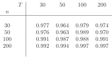
As far as ˆft is concerned, we follow the same logic as in Bai (2003). We compute the correlation coefficient between {fˆt}Tt=1 and {ft}Tt=1, for each Monte Carlo iteration j - sayρ

f

j. We report the average correlation coefficients, i.e. J−1PJ

j=1ρ

f

j, in Table 1 (recall thatJ = 5000).

[Insert Table 1 somewhere here]

Table 1 illustrates that the estimated common factor ˆft is highly correlated with the unobserved common factor ft. This reinforces the results in Bai (2003), albeit obtained in a different context, that the estimated factors are quite good at tracking the true ones; indeed, numerical values are very

similar to those in Table 1 in Bai (2003, p.151). WhennandT are≥100, the estimated factors can

be treated as the true ones.

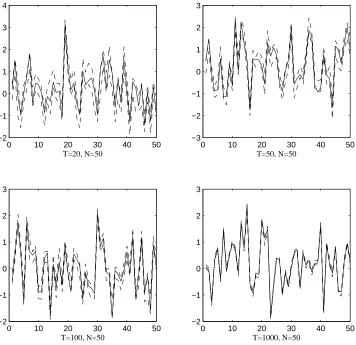
As far as ˆγiis concerned, we report confidence intervals forγi. In order to illustrate how confidence intervals shrink asT expands, we setn= 50 andT = 20,50,100,1000.

According to equation (6) in Theorem 1, as (n, T) → ∞ with √T

n → 0, the 95% confidence interval for H−1_γ

i is given by ˆγi±1√.96_T ×Σˆ1γi/2. Further, let ˆδ be the least square estimate ofδ in Γ = ˆΓδ+error, where Γ = (γ1, . . . γn)′ and ˆΓ = (ˆγ1, ...,ˆγn)′. The 95% confidence interval forγi is therefore obtained as ˆδ×γˆi±1√.96_T ×Σˆ1γi/2

. By rotating ˆγi towardsγi, we consider the confidence interval forγi directly, reported in Figure 1.

[Insert Figure 1 somewhere here]

Figure 1 shows that, in most cases and for all combinations ofnand T, the confidence intervals

contain the true value ofγi. This also holds true for the case (n, T) = (50,1000), where the ratio

√

is not negligible, as the theory would require. As predicted by the theory, asT grows, the confidence

intervals collapse to the true value ofγi.

5.2

Small sample properties -

S

and

S

In this subsection, we report empirical rejection frequencies and power for tests based on the max-type

statisticsSγ,nT andSf,nT defined in (17) and (18) respectively.

As far as the design of the Monte Carlo is concerned, recall that the variance of the common

components cit = γift is set equal to 1 across all experiments. We conduct our simulations for different values of the signal-to-noise ratio V ar_σ(2cit)

ǫ , whereσ 2

ǫ is the variance ofǫit, equal to1₃,1₂,1 . In addition to conducting simulations under the DGP (33), we also consider two alternative

DGPs that are nested in (33), in order to assess the robustness of the tests proposed to different

specifications of (1)-(2). We firstly consider a DGP for the regressorsxit that modifies (34) by not containing common factors, viz.

xit=µi+ǫxit. (35)

In this case, cross dependence in the yits is purely due to the presence of ft in (33). The rank condition in Assumption 3(ii)does not hold, although the CCE estimator is still consistent. Secondly, we consider a DGP for (1) in which there are no unit specific regressors, viz.

yit=γift+ǫit; (36)

this is a pure factor model, that fits in the class of models considered by Bai (2003). In this case, it

can be argued that testing for no factor structure (either by using Sγ,nT orSf,nT) complements the information criteria in Bai and Ng (2002), by being a test for r= 0. This is can also be compared

with the framework in Baltagi, Kao, and Na (2012).

Critical values have been computed by approximating Bn and BT as discussed in Section 3. Unreported simulations show that results worsen only slightly when using the asymptotic critical

values.2

Testing for Ha

0 :γi=γ

When evaluating the empirical rejection frequencies for tests based onSγ,nT, we run the Monte Carlo simulations under the null γi = 1 for alli. When evaluating power, we generate the loadings

γi as i.i.d. N 1, σ2γ

, reporting results for the case of σγ = 0.2. Given that ǫit is cross sectionally uncorrelated and homoskedastic by design, Σγi is estimated as ˆΣγi = ˆσǫ2×T

ˆ

F′_Mx iFˆ

−1

, where

ˆ

σ2ǫ = nT1

Pn i=1

PT t=1ˆǫ2it.

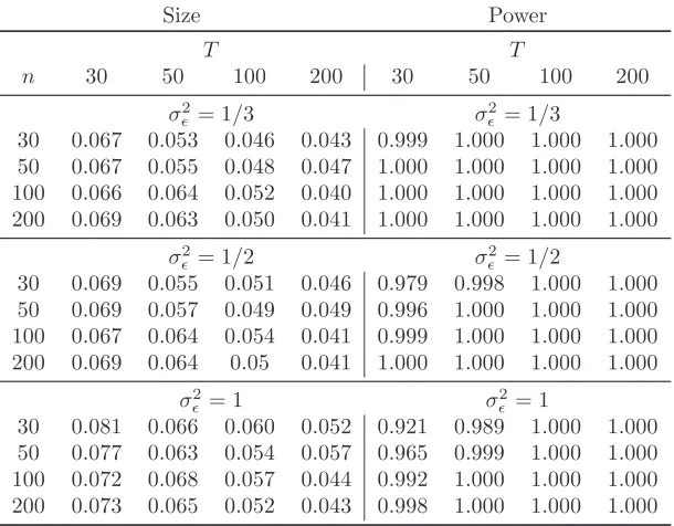
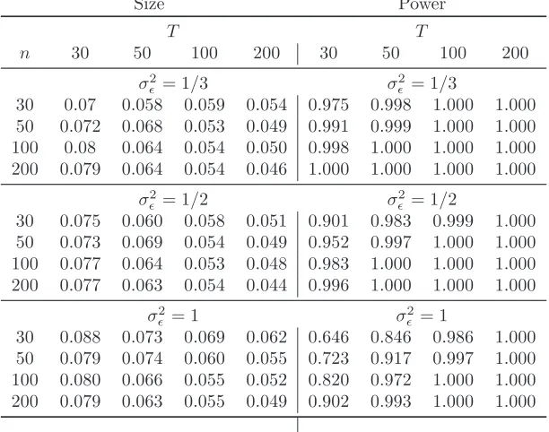
Results for size and power when using the main DGP (33)-(34) are in Table 2.

[Insert Table 2 somewhere here]

We firstly consider the empirical rejection frequencies (left panel in the table). The test has

a tendency to be oversized in small samples; as a general rule, the correct size is attained when

T ≥100 andn≥50; indeed, whenσ2

ǫ = 1 (high signal-to-noise ratio), the test has satisfactory size properties even forT = 50. The Table also shows that, as the signal-to-noise ratio decreases (i.e., as

σ2

ǫ increases), the tendency towards small sample oversizement worsens. This is not so whenT ≥100 andn≥50: the test attains the correct size even for large values ofσ2

ǫ.

As far as the power is concerned (right panel in the Table), the test has good power properties

in all cases: the power is above 50% for almost all cases. We note that, similarly to the size, the

power deteriorates as the signal-to-noise ratio decreases; when n and T are sufficiently large, this

disappears.

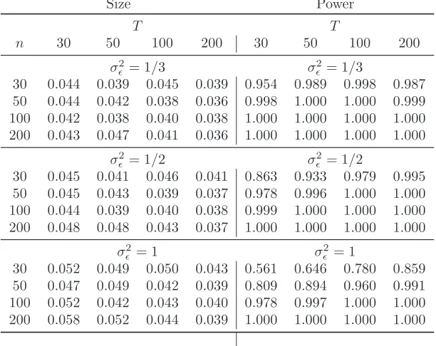
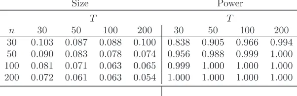
When considering the two alternative specifications (33)-(35) and (36), results are reported in

Tables 3 and 4.

[Insert Tables 3 and 4 somewhere here]

Results do not change much with respect to the ones in Table 2, as far as both empirical rejection

frequencies and power are concerned. Indeed, the size improves in both cases (especially when

simulations are conducted under (36)). When the signal-to-noise ratio is sufficiently high, the test

attains its nominal size for all values ofn, as long asT ≥100.

It is interesting to note that both size and power become much better under (36) than in the

other cases. The correct size is attained as long asn≥30 andT ≥50; moreover, the power is always

above 90% for all combinations of nandT.

We run the Monte Carlo simulations under the nullft= 1 for alltwhen evaluating the size of tests based onSf,nT. When evaluating the power, we generate the common factorsftasi.i.d. N

1, σ2

f

,

reporting results for the case ofσf = 0.2. Finally, we estimate Σf tas Σf t=VnT−1σˆǫ2n1

Pn i=1λˆiλˆ

′

iV−

1

nT where ˆσ2

ǫ = nT1

Pn i=1

PT t=1ǫˆ2it.

Results when using (33)-(34) are in Table 5.

[Insert Table 5 somewhere here]

The size of the test is almost always the correct one, with few exceptions - the test is oversized

for smallT whenσ2

ǫ is high. BothnandT have a quite limited impact on the results.

The test has very good power properties, especially when the signal-to-noise ratio is high. We

note that the power increases with bothnandT, in a more pronounced way withn.

As in the previous subsection, we also considered size and power under the alternative

specifica-tions (33)-(35) and (36); results are in Tables 6 and 7.

[Insert Tables 6 and 7 somewhere here]

Results do not differ much, when carrying out simulations under (33)-(35), from the values in

Table 5. Actually, as it was noted for the case of Sγ,nT, results improve slightly, in particular the power. Similar considerations hold for the empirical rejection frequencies computed under (36): the

size is always the correct one. The power is also very good, under all possible combinations of

parameters.

For the sake of completeness, we run both tests using as a first step estimator the IE proposed

by Song (2013). The size and power reported in Table 8, for the Sγ test, when the DGP is the one in equations (33)-(34), show that the test procedure is unaffected by the choice of the first step

estimator when this is a consistent one.

[Insert Table 8 somewhere here]

In order to assess the finite sample properties of the two test procedures when the errors are

autocorrelated and heteroskedastic, we consider the following DGP:

ǫit= 0.5ǫit−1+uit

uit∼IIDN(0, σui2) σui2 ∼U(0.1,0.5)

and we make use of the HAC estimators for Σγ and Σf given by equations (7) , (10). Apart from these features, the experiments have the same specifications as above. As far as the noise-to-signal

ratio is concerned, results are very similar to the i.i.d. cases, and we only report the cases in which

σ2

ǫ = 1 (i.e. the worst case, based on the simulations above) to save space.

[Insert Tables 9 and 10 somewhere here]

The results in Tables 9 and 10 can be compared with thei.i.d. cases in Tables 2 and 5 respectively. In the case of noni.i.d. errors, both tests have a tendency to be oversized in small samples, (n, T)≤

50. However, as both dimensions are larger than 50, the empirical rejection frequencies become almost

undistinguishable from the ones computed withi.i.d. errors. As far as, the power is concerned, both tests have good properties and are very close to thei.i.d. case.

6

Conclusions

In this contribution, we develop an inferential theory for the unobservable common factors and their

loadings in a large, stationary panel model with observable regressors. Our framework allows for

slope heterogeneity; we also allow for correlation between common factors and observable regressors,

by modelling the DGP of the observable regressors as containing the common factors, in a similar

spirit as in Pesaran (2006).

We extend the framework in Pesaran (2006) by providing a two stage estimator for the unobserved

common factors and their loading. We derive rates of convergence and limiting distribution of both

the estimated factors and loadings, using a similar method of proof to Bai (2009a). In a similar

vein to Sarafidis, Yamagata and Robertson (2009), we also develop two tests for the null of no

factor structure, based on the null that factor loadings are homogeneous, and that common factors

are homogeneous over time, respectively. In either case, the assumed factor model boils down to

can be captured by inserting time dummies or unit specific dummies. The proposed test procedures

simplify the specification analysis of heterogeneous panel data models with unobserved factors. From

a methodological perspective, this entails that the tests can be implemented without prior knowledge

of the number of factors. The only thing which is needed is a consistent preliminary estimation of the

slope parameters. Building on this, we propose statistics based on extrema of the estimated loadings

and common factors. Under the null, the test statistics converge to an Extreme Value distribution.

As far as power is concerned, from a theoretical point of view our tests are consistent even under

alternatives where only one loading or common factor differs from the average. Monte Carlo evidence

shows that both tests have the correct size and good power properties.

Building on the theory developed in this paper, there are several interesting avenues for further

developments. An important case is the estimator of theβis used in Step 1. In our paper, we focus on the CCE estimator proposed by Pesaran (2006); this estimator is easy to treat analytically, but it is

only a possible choice. In particular, our setup requires strict exogeneity, thereby ruling out e.g. the

possibility of having lagged values of the yits among the regressors. This requirement is due to the estimation method employed in Step 1, rather than to the inference on factors and loadings per se.

Indeed, the CCE is known not to work in presence of weakly exogenous regressors (see Everaert and

Groote, 2012; and Chudik and Pesaran, 2013). However, the assumption of strict exogeneity can be

readily relaxed (accommodating e.g. for dynamic models), upon employing, in Step 1, an estimator

of the βis that is consistent at a rateOpminT−1/2, n−1 . A possible choice for this case is the IE estimator studied in Song (2013), which has the desired convergence rate, even in presence of

dynamic models. Alternatively, a different approach, based on unit specific estimators can be used,

by instrumenting the unobservable common factors ft using the regressorsxjt for each uniti, with

i 6=j - indeed, both the CCE and the IE have a natural Instrumental Variable interpretation (see

also Bai, 2009b). Such extensions are currently under investigation of the authors.

Acknowledgement

This is a revised version of a paper previously circulated under the working title “Two-Stage

Inference in Heterogeneous Panels”. We are very grateful to the Editor (Cheng Hsiao), one

anony-mous Associate Editor and two anonyanony-mous Referees for very constructive feedback which has greatly

improved the generality of the paper. We also wish to thank the participants to the Faculty of

Finance Workshops at Cass Business School; to the New York Camp Econometrics V (Syracuse

Financial Econometrics (London, December 2010); to the 18th International Conference on Panel

Data (Banque de France, July 2012), in particular Chihwa Kao, Jean-Pierre Urbain and Takashi

Yamagata. Special thanks go to Lajos Horvath for providing us with valuable comments. The usual

Appendix A: Technical Lemmas

In this Appendix and the next one, we setH =Irin the proofs (although not in the statements of the Lemmas), for the sake of notational simplicity. Inequalities are written, when possible, omitting

constants.

The Lemmas in this Section extend various results in Bai (2009a,b) to our framework. All proofs

rely upon the decomposition - see Proposition A.1 in Bai (2009a):

ˆ

F−F = 1

nT n X j=1 Xj ˜

βj−βj β˜j−βj

′

Xj′Fˆ (37)

−_nT1

n X j=1 Xj ˜

βj−βj

γj′F′Fˆ− 1 nT n X j=1 Xj ˜

βj−βj

ǫ′jFˆ

−_nT1

n

X

j=1

F γj

˜

βj−βj

′

Xj′Fˆ− 1 nT n X j=1 ǫj ˜

βj−βj

′

Xj′Fˆ

+ 1

nT

n

X

j=1

F γjǫ′jFˆ+ 1

nT

n

X

j=1

ǫjγj′F′Fˆ+ 1

nT

n

X

j=1

ǫjǫ′jF .ˆ

In (37), the main difference with Bai (2009a) is the presence of the unit specific estimates, ˜βj. Consider also the following notation, which we use henceforth throughout Appendices A and B. We

define Υi≡ Xi′M¯wXi−

1

X′

iM¯wǫi, so that we can write

˜

βi−βi =

Xi′M¯wXi

T

−1

Xi′M¯wǫi

T

+

Xi′M¯wXi

T

−1

Xi′M¯wF

T γi

(38)

= Υi+ ¯Υi,

for every i; by construction, ¯Υi = Op 1_n+Op

1 √

nT

. We extensively use the notation δnT = minn√n,√ToandφnT = min

n

n,√To.

Lemma A.1Under Assumptions 1-4, it holds that, for every i,Eβ˜i−βi

r

=O φ−nTr

, for any

r≤3.

Proof. Let kAk1 denote theL1-norm of a matrix A, i.e. kAk1 = maxx6=0kAxk1/kxk1. By a

well known norm inequality (see e.g. Strang, 1988, p. 369, exercise 7.2.3), it holds that

β˜i−βi

r ≤ _X′

iM¯wXi

T −1 r 1 X ′

iM¯wǫi

T +

X′

iM¯wF

T γi

r =

l−_min1

_X′

iM¯wXi

T r X ′

iM¯wǫi

T +

X′

iM¯wF

T γi

where the last equality holds by symmetry. In view of Assumption 4(i), and omittingγiby virtue of Assumption 3(iii)

Eβ˜i−βi

r ≤E X ′

iM¯wǫi

T r +E X ′

iM¯wF

T r

=I+II.

ConsiderI; we haveI≤T−r_EkX′

iǫikr=T−rE

PTt=1xitǫit

r. It holds that

T−rEkXi′ǫikr ≤ T−rE

T X t=1

kxitǫitk2

r/2

≤T−rE

T

1−2/r T

X

t=1

kxitǫitkr

!2/r

r/2 (39)

≤ T−rTr/2 1 T

T

X

t=1

Ekxitǫitkr

!

≤T−r/2 1 T

T

X

t=1

h

Ekxitk2r

i1/2h

E|ǫit|2r

i1/2!

= OT−r/2_,

where we have used: Assumption 2(iv); Holder’s inequality; theCr-inequality and Jensen’s inequality; the Cauchy-Schwartz inequality; and the fact that, by Assumptions 1 and 2(i), E|ǫit|2r <∞ and

Ekxitk2r < ∞ respectively. Using the Cauchy-Schwartz inequality in this context is more than what is necessary, since xit and ǫit are independent. Turning to II, note that, for sufficiently large n and omitting higher order terms, H¯′

wH¯w−

1

= D−1

w −Dw−1RwDw−1, with Dw = C′F′F C and kRwk = Op 1_n+Op

1 √

nT

- see e.g. equation (29) in Pesaran (2006). Therefore, letting

¯

ǫ=n−1Pn

i=1ǫi and omitting higher order terms

X′

iM¯wF

T = −

X′

iF CDw−1¯ǫ′F

T2 −

F′_¯ǫD−1

w C′F′Xi

T2 (40)

−Xi′¯ǫD−

1

w ¯ǫ′F

T2 −

X′

iF CD−w1RwD−w1C′F′F

T2

= −I−I′−II−III.

ConsiderEkIkr; sinceC has full rank by Assumption 4(ii) andDwis invertible

EkIkr≤E

X ′ iF T ¯

ǫ′_F

T r ≤M " E X ′ iF T

2r#1/2"

E ¯ǫ ′_F T

2r#1/2

.

Consider the first term; we have T−1PT

t=1Ekxitft′k

2r

≤ T−1PT t=1

h

Ekxitk4r

i1/2 h

Ekftk4r

i1/2

which is finite by Assumption 2(i). As far as the second term is concerned, note E ¯

ǫ′_F

T 2r

≤T−2r

T

X

t=1

h

Ekftk4r

i1/2

 E 1 n n X i=1 ǫit

4r



1/2

,

after similar passages as in equation (39). It holds that Ekftk4r < ∞ by Assumption 2(i). By using Assumption 1(iv)(b) and following thereafter a similar logic as in the proof of (39), we have

E1

n

Pn i=1ǫit

4r

=O n−r/2_{, so that EkIk}r

=O n−r/2_T−r/2_{. The same logic yields EkIIk}r =

O(n−r_T−r_{). Finally, considerIII; after some passages}

EkIIIkr≤ kRwkr

" E X ′ iF T

2r#1/2"

E F ′_F T

2r#1/2

=O(kRwkr),

again by similar passages as above. Therefore, EXi′M¯wF

T

r = O(kRwkr). Putting everything together, the Lemma follows. QED

Lemma A.2Under Assumptions 1-4, it holds that, for every i

A.2(i) T−1_ǫ′

i

ˆ

F−F=Op δnT−2

;

A.2(ii) n−1/2_T−1Pn i=1ǫ′i

ˆ

F−F=Op n−1/2+Op T−1.

Proof. The proof of A.2(i) is very similar, and in fact simpler, than that of A.2(ii); thus we focus on the latter only. Using (37)

n−1/2T−1

n

X

i=1

ǫ′i

ˆ

F−F (41)

= 1

n√T

n

X

j=1

Pn i=1ǫi √_n ′ Xj √ T ˜

βj−βj β˜j−βj

′X′

jFˆ

T −

1

n√T

n

X

j=1

Pn i=1ǫi √_n ′ Xj √ T ˜

βj−βj

γ′

j

F′_Fˆ

T

−_nT1

n

X

j=1

Pn i=1ǫi

√ n ′ Xj √ T ˜

βj−βj

_ǫ′

jFˆ

√

T −

1

n√T

Pn i=1ǫi

√ n ′ F √ T n X j=1 γj ˜

βj−βj

′X′

jFˆ

T

−√1

n 1 nT n X j=1 n X i=1 ǫ′

iǫj

˜

βj−βj

′X′

jFˆ

T + 1 √ nT 1 √ n n X i=1 ǫ′ iF √ T 1 √ n n X j=1 γj ǫ′

jFˆ

T

+√1

nT 1 √ n n X i=1

ǫ′i 1 √ n n X j=1

ǫjγ′j

F′_Fˆ

T + 1 T 1 n n X j=1 Pn i=1ǫi

√

n

′

ǫj

ǫ′

jFˆ

T

The proof follows very similar lines to that of Lemma A.8 in Song (2013): the only difference is

the different expansion of the estimation error ˜βj−βj when using the CCE. Thus, we report only the complete passages to determine the order of magnitude of I; the same logic applies to all the other

terms in the expansion. The only term for which passages slightly differ isV, and we report the full

blown proof for it.

ConsiderI; it holds thatI≤n−1Pn j=1

Pn i=1ǫ′iXj

√_nT X ′

jFˆ

T β˜j−βj

2

. This is bounded by

E " Pn i=1ǫ′iXj

√_nT X′

jFˆ

T β˜j−βj

2 # (42) ≤ E β˜j−βj

2p

1/p"

E

Pn i=1ǫ′iXj

√ nT X′

jFˆ

T

!q#1/q

≤

Eβ˜j−βj

32/3"

E Pn i=1ǫ′iXj

√_nT

6#1/6

E X′

jFˆ

T 6 

1/6

,

using Holder’s inequality in the first line (withp= 3

2 andq= 3), and the Cauchy-Schwartz inequality

in the second line. The first term is of order O φ−_nT2in light of Lemma A.1. Similar passages as in the proof of Lemma A.1 yield that both the second and third terms are of order O(1). This

entails thatI =Op T−1/2φ−nT2

. Similar passages yieldII =Op T−1/2φ−nT1

; III =Op T−1φ−nT1

;

IV =Op T−1/2φ−_nT1; V I =Op T−1/2φ−_nT1+Op δ−_nT2;V II =Op n−1/2andV III =Op T−1 +Op n−1/2T−1/2.

Consider nowV, whose proof is marginally different to that of Song (2013)

V ≤  1 n n X j=1 E 1 √ nT n X i=1 T X t=1

ǫitǫjt

2 

1/2

1 n n X j=1 E X′

jFˆ

T β˜j−βj

!2



1/2

≤  1 n n X j=1 E 1 √ nT n X i=1 T X t=1

ǫitǫjt

2 

1/2

1

n

n

X

j=1

Eβ˜j−βj

3  

1/3

1 n n X j=1 E X′

jFˆ

T 6 

1/6

=   1 nT n X j=1 E 1 √ nT n X i=1 T X t=1

ǫitǫjt

2 

1/2

Op φ−nT1

,

using the Cauchy-Schwartz inequality (first line), Holder’s inequality with the same orders as in (42)

(second line) and Lemma A.1. Also, E_√1

nT

Pn i=1

PT t=1ǫitǫjt

2

≤(nT)−1 Pn_i=1 Pn_j=1 PT_t=1 PT_s=1

|E(ǫitǫktǫjsǫks)| ≤ M, by Assumption 1(iii)(d), so thatV =Op T−1/2φ−nT1

. Putting all together,