The generative learning and discriminative fitting of linear deformable models

(1)

The Generative Learning and

Discriminative Fitting of Linear

Deformable Models

Jason Mora Saragih

A thesis submitted for the degree of Doctor of Philosophy of The Australian National University

1 October 2008

Research School of Information Sciences and Engineering The Australian National University

(2)

(3)

Declaration

This thesis describes the results of research undertaken in the Department of Information En-gineering, Research School of Information Sciences and EnEn-gineering, The Australian National University, Canberra. This research was supported by scholarships from the Australian Re-search Council under the Australian Postgraduate Awards (Industry) (APAI) and The Aus-tralian National University, Canberra.

The results and analyses presented in this thesis are my own original work, accomplished under the supervision of Doctor Roland G ¨ocke, Doctor Hongdong Li and Doctor Nick Barnes, except where otherwise acknowledged. This thesis has not been submitted for any other degree.

Jason Saragih

Department of Information Engineering

Research School of Information Sciences and Engineering The Australian National University

Canberra, Australia 1 October 2008

(4)

(5)

Acknowledgements

I would like to express my deep and sincere gratitude to my supervisor Dr. Roland G ¨ocke for his unrivalled guidance and patience throughout the course of this study. His never-ending optimism and encouragement has been a guiding beacon in the rough-and-tumble of false starts and ideas that went pear-shaped. The lengths to which he helped was truly momentous and perhaps unprecedented. For this and more, I am truly grateful.

I would also like to thank my family for all their support and understanding during this period. To my parents, for providing space and shelter for me to pursue my studies. To my sisters, Vera and Melissa, for keeping my feet firmly grounded. To my brother, Jordan, for keeping me physically active as well as for the occasional comic relief. Also, to my cousins Vina and Meta, for the much needed nutrition.

My deepest gratitude also to Junko for her love, companionship and above all, patience, during this time. Her cheerful disposition and comforting demeanour proved irreplaceable though the numerous highs and lows.

Also, many thanks to my brothers and sisters in arms: Dave, Tal, Jill, Karl, Shawn and all those who joined in on getting down. Those were truly times to remember. Special thanks goes out to Dave and Tal, for their skewed personalities and hilarious perspectives, which made light of dilemmas and deflated misplaced immodesty.

I would also like to thank Dr. Hongdong Li, Dr. Nick Barnes and Prof. Richard Hartley for taking the time to humour my naive ideas. I found the numerous discussions we had to be enlightening and very instructive through the struggle to understand and go beyond.

Last but not least, I would like to thank Dr. David Austin for guiding me through the first years of my studies as well as giving me the opportunity to pursue this work to begin with.

(6)

(7)

Abstract

The recovery of a deformable visual object’s structure from an image is a central problem in computer vision. It is often tackled through the utility of a Linear Deformable Model (LDM), which models variations of a visual object’s shape and appearance linearly. This model has been shown to exhibit excellent modelling capacity whilst affording a compact representation of variability. However, it suffers from two major drawbacks. Firstly, there are significant difficulties regarding data collection, where a large number of correspondences is generally required in order to build the statistical models of shape and appearance that parameterise the LDM. The manual annotation of large databases can therefore be tedious and error prone. Secondly, approaches for structure recovery must address the conflicting goals of accuracy, reliability and efficiency.

In this thesis, contributions are made to address these two major areas of difficulty. In the first, the problem of automatic correspondence learning between pairs of images is tackled from a Bayesian perspective. The result is a general approach that allows domain knowledge to be integrated directly into the problem, where adaptations to similar problems are afforded through an explicit derivation of the involved components. In the second area of difficulty, the compromise between accuracy, reliability and efficiency in structure recovery is addressed through a generic method coined the iterative-discriminative approach. Leveraging on the predictive capacity of discriminative methods and the iterative framework of generative fitting, the approach is shown to exhibit excellent accuracy and reliability whilst also affording the most efficient procedure for LDM fitting known to date.

The problem of automatic correspondence learning is posed as a direct pairwise registra-tion problem. Within its Bayesian formularegistra-tion, it utilises the method of Hierarchical Priors in order to allow parameterisations of the involved densities to be optimised in conjunction with the correspondences. This is a significant step away from conventional approaches that utilise a fixed parameterisation, requiring a tedious cross validation procedure to determine the best parameterisation for a particular problem. Furthermore, the proposed approach introduces an objective criterion with which the quality of the found correspondences can be evaluated. Op-timisation of the parameterisation and correspondences is achieved through the marginalised

maximum likelihood/maximum a posteriori procedure that alternates between optimising the

likelihood of the data with respect to the parameterisation (with marginalisation taken over the correspondences) and optimising the posterior of the correspondences for a fixed estimate of the parameterisation. The efficacy of the proposed approach is evaluated for the case of the human face on three types of databases: person specific, pose specific and generic person databases.

The iterative-discriminative approach for LDM fitting makes use of a novel fitting objec-tive in its training procedure called error bound minimisation. This objecobjec-tive places emphasis on the gradual reduction of the spread of training samples about their respective optimum by

(8)

minimising the bound over the perturbations of the training data at each iteration. Since the objective only needs to be partially satisfied at each iteration, this approach allows simple re-gressors to be utilised, which exhibit better efficiency and generalisability in comparison to more complex ones. Four prototypes of the iterative-discriminative approach are proposed in order to tackle the problems of linear fitting, nonlinear fitting, robust fitting and background in-variant fitting. The efficacy of the proposed prototypes is evaluated with regard to the problem of generic face fitting.

(9)

Publications

During the course of this study, the following refereed conference papers were published.

• Jason Saragih and Roland Goecke, “A Nonlinear Discriminative Approach to AAM Fitting”. In Proceedings of the Eleventh IEEE International Conference on Computer

Vision ICCV 2007, Rio de Janeiro, Brazil, 14–20 October 2007. IEEE.

• Jason Saragih and Roland Goecke, “Monocular and Stereo Methods for AAM Learning from Video”. In Proceedings of the IEEE Computer Society Conference on Computer

Vision and Pattern Recognition CVPR2007, Minneapolis (MN), USA, 18–23 June 2007.

IEEE.

• Shaun Press, Jason Saragih and Jason Chen, “Eye contact as a key component in Human Robot Interaction”. In Proceedings of the 2006 Australasian Conference on

Robotics and Automation ACRA2006, Auckland, New Zealand, 6–8 December 2006.

• Jason Saragih and Roland Goecke, “Learning Active Appearance Models from Im-age Sequences”. In Proceedings of the HCSNet Workshop on the Use of Vision in HCI

VisHCI2006, volume 56, pages 51-60, Canberra, Australia, 1–3 November 2006. ACS.

• Jason Saragih and Roland Goecke, “Iterative Error Bound Minimisation for AAM Alignment”. In Proceedings of the 18th International Conference on Pattern

Recog-nition ICPR2006, volume 2, pages 1192-1195, Hong Kong, China, 20–24 August 2006.

IEEE.

(10)

(11)

Abbreviations

AAM Active Appearance Model

ASM Active Shape Model

ATLID Asymptotically Trained Linear Iterative-Discriminative BFGS Broyden-Fletcher-Goldfarb-Shanno

BIID Background Invariant Iterative-Discriminative

COTLID Constrained Optimisation Trained Linear Iterative-Discriminative C-RIC Commensurate Robust Inverse Compositional

EM Expectation Maximisation

FJ Fixed Jacobian

GMM Gaussian Mixture Model

HFBID Haar-like Feature Based Iterative-Discriminative

ICA Independent Component Analysis

ID Iterative-Discriminative

KPCA Kernel Principal Component Analysis

LDM Linear Deformable Model

MAP Maximum A Posteriori

MDL Minimum Description Length

ML Maximum Likelihood

MML Marginalised Maximum Likelihood

MRI Magnetic Resonance Imaging

NC-RIC Non-Commensurate Robust Inverse Compositional NIC Normalised Inverse Compositional

PCA Principal Component Analysis

PDF Probability Density Function POIC Project-Out Inverse Compositional

PPCA Probabilistic Principal Component Analysis

RAM Random Access Memory

RGB Red Green and Blue

RIC Robust Inverse Compositional RID Robust Iterative-Discriminative

RMS Root Mean Squared

SAT Summed Area Table

SIC Simultaneous Inverse Compositional SVD Singular Value Decomposition

SVR Support Vector Regression

3DMM 3D Morphable Model

(12)

(13)

List of Figures

1.1 Structure recovery as a preprocessing step. . . 2

1.2 Schema of linear model building. . . 3

1.3 An illustration of analysis-by-synthesis. . . 4

2.1 Homologous point set example. . . 10

2.2 Examples of intrinsic shape variation. . . 11

2.3 Example of shape eigenspectrum. . . 13

2.4 Illustration of appearance synthesis in an LDM. . . 16

2.5 Example of intrinsic appearance variations. . . 17

2.6 Example of combined appearance variation. . . 18

2.7 Schema of generative LDM fitting. . . 27

3.1 Example IMM images with bounding box. . . 36

3.2 Examples of piecewise smooth variations. . . 42

3.3 Examples of prior penalisers . . . 42

3.4 The IMM Face database. . . 55

3.5 Example of correspondence initialisation . . . 56

3.6 Illustration of the hyperparameters convergence. . . 57

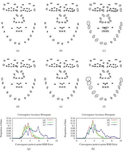
3.7 Performance of the pairwise method on person specific databases starting from optimal correspondences . . . 59

3.8 Performance of the pairwise method on person specific databases using box detected initialisation . . . 60

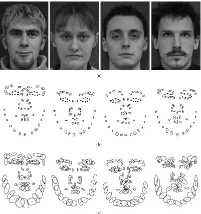
3.9 Reconstruction results of intra-person pairwise learning. . . 61

3.10 Results for pose specific databases. . . 63

3.11 Performance of the pairwise method on a pose specific database, starting from optimal correspondences . . . 64

3.12 Reconstruction results of inter-person pairwise learning. . . 65

3.13 Performance of the pairwise method on a generic person database, starting from optimal correspondences . . . 67

4.1 Illustration of IEBM process. . . 79

4.2 Objective functions used in iterative-discriminative fitting, along with the quadratic penaliser. . . 82

5.1 Performance comparisons between the non-robust baseline AAM fitting methods.103 5.2 Effects of initialisation on convergence accuracy on FJ, POIC, SIC and NIC. . . 104

5.3 Examples of the normalised raw cropped image features . . . 105

(18)

5.4 Convergence performance of the linear method trained on four settings of the

regularisation parameterλ. . . 106

5.5 Performance comparison between ATLID, COTLID and FJ . . . 107

5.6 Distribution of the training samples of the IMM database throughout HFBID’s training process . . . 109

5.7 Convergence performance of HFBID. . . 110

5.8 Performance comparisons between HFBID, COTLID and FJ . . . 111

5.9 Examples of synthetically occluded images . . . 112

5.10 Convergence performance of RID, trained on four different settings of the reg-ularisation parameterλ. . . 113

5.11 The effects of assuming spatially coherent occlusions in RIC. . . 115

5.12 Performance comparisons between the RID, C-RIC and NC-RIC. . . 116

5.13 Chrominance based background segmentation. . . 118

5.14 The evolution of features chosen for inclusion throughout the fitting procedure of BIID . . . 119

5.15 Performance evaluation of BIID on three different backgrounds . . . 120

A.1 Piecewise affine warp illustration. . . 132

C.1 The pairwise learning executable configuration for the executablepwlearn. . 156

C.2 An example configuration file for themarkupapplication. . . 156

C.3 An example configuration file for thegetbbapplication. . . 157

C.4 Thecam visualiseapplication. . . 157

(19)

List of Tables

3.1 Person specific experiments with manual initialisation . . . 57

5.1 Appearance Model Details for 4-fold Cross-validation . . . 102

5.2 Summary of the Synthetically Occluded Results . . . 117

C.1 LDM Modelling Classes . . . 153

C.2 AAM Fitting Methods . . . 154

C.3 Miscellaneous Classes . . . 155

C.4 Executables . . . 155

(20)

(21)

The beginning is the end is the beginning.

Smashing Pumpkins

Chapter 1

Introduction

1.1 Motivation

Our world is not a rigid place. Many objects that we encounter in our daily lives exhibit inherent deformabilities. Understanding the deformations of these deformable objects has, therefore, proven vital in the advancement of many technological ventures.

Computer vision, a field that studies methods to understand images through the automatic recovery of their structure and its interpretation in the context of a problem, must therefore account for these deformations. In fact, due to the limited observatory power of images, even rigid 3D objects can appear to exhibit deformations in an image due to their projection onto the image as a visual object. Here, interpretation denotes the extraction of high level information from image structure, which defines the image’s partitioning, functional properties and their relations to each other. For example, in the context of facial interpretation, this may involve the extraction of high level information such as: Is there a face in the image? Is it male or female? What is his/her emotional state? Who is it? In this case and many more, perhaps the most influential issue, which affects the possible deployment of computer vision applications on real world problems, is the recovery of the image’s underlying structure, which can be thought of as a preprocessing step to image interpretation (see Figure 1.1). The deformations inherent in many interesting objects adds a degree of difficulty to structure recovery from images.

In the past, many attempts have been made that utilise only a coarse structure recovery process for image interpretation. Such methods, which generally utilise powerful and well de-veloped machine learning algorithms such as Neural Networks and Support Vector Machines, embed a large proportion of the variations exhibited by these deformable visual objects into the interpretation process. Examples of these for face recognition can be found in [57; 69]. Although some impressive results have been reported using this approach, implementation dif-ficulties inherent in these methods have restricted their usage for large scale deployment. One of the major sources of difficulty in this holistic interpretation approach is that deformations introduce nonlinearities into the visual object’s appearance. For example, when structure re-covery only involves the detection of an object’s location and scale, the functional variation in pixel values within a rectangle containing a projected 3D object as it rotates follows a non-linear appearance manifold in pixel space [95]. In order to gain sufficient accuracy for real world applications, there needs to be a large corpus of training data containing images of the object at an extensive range of poses. Although sufficiently large collections of training data are now available for many interesting problems, the extra nonlinearities caused by the inherent

(22)

Image Interpretation

Structure Recovery Expression Transfer

Avatar Animation

Graphics Applications

Appearance Shape Fitted Image

Female

Smiling

Nicole Identity

Expression Gender

Figure 1.1: Structure recovery as a preprocessing step to image interpretation and graphics applications.

Face images taken from the IMM Face Database [89].

variabilities of a visual object mean that interpretation usually involves a highly sophisticated nonlinear learner that can be computationally expensive to evaluate online. For real world ap-plications that require a number of different interpretations of the same image, for example simultaneous visual speech and expression recognition, this approach can quickly become in-feasible. Furthermore, the complexity of the predictive functions in the interpretation process often gives rise to generalisability problems.

In recent years, deformable models have enjoyed much attention in the computer vision community as a way to handle deformabilities of visual objects. This group of approaches utilises a more sophisticated structure recovery mechanism, where deformations are explic-itly accounted for through model parameterisation. Deformation induced nonlinearities in the structure can then be accounted for by the interpretation process through structure normalisa-tion. Throughout the years, some ingenious parameterisations and their utility have been pro-posed, such that the applicability of deformable models is now widespread in human-computer interaction [59; 138; 140], medical image analysis [98; 132; 148] and industrial vision [28; 39; 87].

The computer graphics community has also benefited from the development of deformable models. In this field, the recovered deformable structure is not used to normalise some data to be interpreted, but rather it is used explicitly for image synthesis. Examples of this include facial expression transfer [101; 136], avatar animation [77], visual speech synthesis [120] and face de-identification [56] (note that some of these applications involve a crossover with com-puter vision). In many applications in this field, the use of deformable models has allowed the automation of many tasks (see [19], for example), which previously required treatment by a human expert, significantly reducing workload as well as increasing efficiency.

(23)

[image:23.612.135.501.67.274.2]

§1.2 Objectives 3

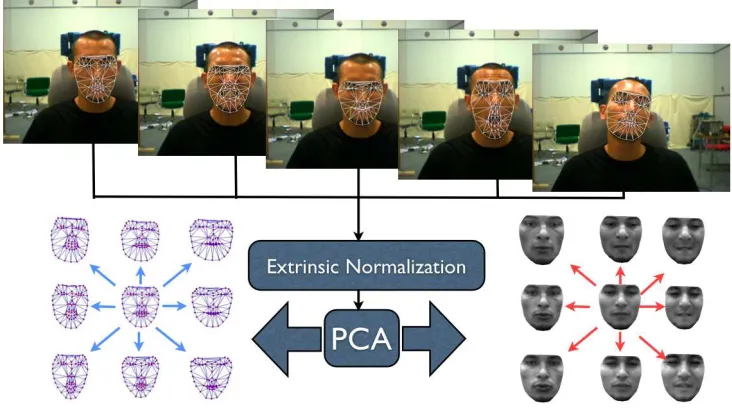
Figure 1.2: An illustration of the LDM learning process along with its various components. From a

set of annotated training images, separate linear models of shape and appearance are learnt through principle component analysis (PCA).

between the synthesised model’s appearance and that of the image (see Figure 1.3 for an illus-tration). Although any deformable visual object can be modelled by an LDM, it is particularly well suited to modelling visual objects whose variations live in a much smaller subspace than their representation. Examples of objects that exhibit this kind of variability include numerous anatomical structures, such as the human face [30]. One of the main strengths of LDMs is their compact representation of complex deformations by modelling the major directions of variations within the constrained subspace of variability.

1.2 Objectives

(24)

Figure 1.3: An illustration of analysis-by-synthesis on an image taken from the IMM Face Database [89]. Left to right: Input image, initial model estimate, recovered structure after 5 itera-tions, recovered structure at convergence. Note that the RGB channels of the model are reversed (i.e. BGR) to highlight the model from the image.

generally account for occlusions or unmodelled variabilities, which are commonly encountered in real world applications, dramatically limiting the scope of these methods.

The primary goal of this thesis is to at least partially address the two major drawbacks of the LDM as described above. To address the problem of data collection, the utility of direct

pair-wise methods for automatic correspondence learning is rigorously investigated. Formulated

within a Bayesian framework, a number of assumptions regarding the generative properties of deformable model matching, a component of the generative correspondence learning problem, as well as the distribution of their deformations, are investigated in a principled manner. The Bayesian framework adopted here also allows all the free parameters within the problem to be tuned automatically. This is a problem that has been largely ignored in most existing works. It will be shown that the regularised data fitting problem, which is the formulation often used in existing works, can be derived directly from a Bayesian formulation, and that it constitutes the case where the parameterisations of the densities involved in the Bayesian formulation are known and fixed. Through extensive empirical evaluations on the human face, the direct pairwise method for automatic correspondence learning is shown to be capable of modelling typical variations such as pose, lighting, expression and identity. However, it is also discov-ered that the method is highly sensitive to initialisation, where optimisation often terminates in a local minimum. Nonetheless, the Bayesian framework presented here serves as a flexible method from which further studies can benefit. An example of the adaptation of the proposed procedure as a groupwise method, where the linear models of the LDM’s shape and appearance are learnt along with the correspondences, is also presented in this dissertation.

(25)

§1.3 Overview 5

discriminative methods. Training on simulations of real fitting problems, it is shown that this approach exhibits excellent generalisability on unseen instances of the visual object as well as affording a flexibility in the level of desired accuracy, which can be tuned based on the needs of the image interpretation application that uses its recovered structure. This is achieved through the concept of iterative error bound minimisation, whereby at each iteration of the algorithm computational resources are focused primarily on tackling the worst case scenarios, minimis-ing the errors on simulated samples that are furthest from their desired settminimis-ings. By virtue of its iterative framework, the discriminative predictors (regressors) need only partially satisfy the problem’s objective at each iteration, since the continuity of objective between iterations gives rise to further overall improvements in future iterations. As such, the approach affords the utilisation of simple functional forms for its predictors, which generally exhibit better gen-eralisability than their more complex counterparts, as well as affording a rapid evaluation. The approach proposed here is also highly applicable, as instances can be created using a variety of model parameterisations, regressors and feature extraction procedures (that are used to drive the regressors). As such, a number of prototypes of this approach will be evaluated in this dissertation, highlighting its applicability. These prototypes include those that utilise linear and nonlinear regressors as well as one that is robust in the presence of occlusional effects. An extension of the linear prototype that can handle varying backgrounds is also presented, where it is shown that background invariance can be achieved without sacrificing performance.

A secondary goal of this dissertation is to provide a flexible software framework that builds on fixed parameterisations of the various flavours of LDMs, where extensions and develop-ments in any aspect of their application can be easily augmented. For this, the Deformable Model Library (DeMoLib), a C++ Application Programming Interface (API) for deformable model learning and fitting, is provided along with this dissertation. A number of components commonly used by LDMs can be found here, such as linear shape and appearance model classes, warping and various other geometric functions (Procrustes alignment, for example), as well as full implementations of a number of prominent AAM and ASM fitting procedures. The API also provides a Graphical User Interface (GUI) for a number of common tasks, such as manual annotation, linear model viewing, and visualisation of model fitting and tracking procedures. Although a number of similar libraries now exist, most have their drawbacks. The AAM API [113], for example, implements only the original AAM fitting procedure and is plat-form dependent (i.e. it is a Windows only API). Another example isam tools1, for which the source code is not publicly available. In contrast,DeMoLibis a platform independent API whose source code is made publicly available for research purposes. Finally, it should be noted that all experiments presented in this dissertation were implemented usingDeMoLib, allow-ing reproduction of all results usallow-ing the publicly available database on which the experiments were conducted.

1.3 Overview

This dissertation is comprised of six chapters, the first of which is this introduction. The chapters are organised in such a way that the reader will benefit by reading the chapters in

1

(26)

order as conventions and terminology set out in earlier chapters are adopted in the chapters that follow. This is especially the case for Chapters 4 and 5, where the latter is an empirical evaluation of the former. However, the problems tackled in Chapters 3 and 4, as well as their proposed solutions, are separate and distinct. As such, the reader can freely interchange the order of these chapters, but is strongly encouraged to first read Chapter 2.

A brief outline of each of the chapters that follow is given below:

Chapter 2 comprises a general overview of LDMs. This includes a detailed discussion of their common parameterisations and a brief outline of some less common representa-tions. The models described in this chapter serve as a basis for the prototypes used in the experiments of LDM fitting, presented in Chapter 5. A review of existing meth-ods for automatic correspondence learning for LDM building is also presented, where the strengths and weaknesses of some of the more prominent methods are discussed. Fi-nally, a taxonomy of existing LDM fitting approaches is presented, grouping the methods based on their algorithmic realisations.

Chapter 3 presents a rigorous investigation into the utility of direct pairwise approaches for automatic correspondence learning. The formulation of the problem within a Bayesian framework is derived along with a discussion of possible parameterisations for the in-volved densities. The applicability of the approach is empirically evaluated through experiments on a face database, testing its performance for person specific, pose specific and generic person models. Analysis of the results is presented along with suggestions for further improvements.

Chapter 4 presents the iterative-discriminative approach for LDM fitting, a novel approach that leverages on the predictive capacity of discriminative methods and the iterative framework of generative fitting, coupled through the objective of error bound minimi-sation. Details regarding its derivation as well as the motivating factors involved are discussed with reference to existing fitting approaches. Several prototype methods are presented that utilise linear and nonlinear regressors as well as extensions that can handle occlusions and varying backgrounds.

Chapter 5 comprises an investigation into the efficacy of the iterative-discriminative approach through experiments on the various proposed prototypes. Empirical evaluations are per-formed on the difficult problem of generic face fitting with comparisons made against a number of existing methods for LDM fitting. Analyses of the results are presented along with ideas for further performance gains.

Chapter 6 concludes this dissertation with an overview of contributions and mention of di-rections for future work.

1.4 Mathematical Nomenclature

(27)

§1.4 Mathematical Nomenclature 7

Scalars are written in italics, either in lower or upper-case, for example:aandB.

Vectors are written in lower-case non-italic boldface, with components separated by spaces, for example:

v=a b cT = [a; b; c] =

  a b c  =   a b c   (1.1)

is a column vector, whereT denotes the vector or matrix transpose. The type of brackets is chosen in the context of an equation to clarify the exposition. Elements of a vector are represented by the lower-case italic vector name with a parenthesised index as its subscript. For example: v₍_i₎ is the ith _{element of vector} _v_{. The size of a vector is}

represented by a parenthesised number as its superscript, for example: v(n) is an n -length vector. Sub-vectors are represented by the range in the indices, for example:

v_(2:5) denotes the 4-length vector comprising of elements 2 to 5 ofv inclusive. If no starting or ending index is specified, then the sub-vector consists of elements to the beginning or end of the vector, respectively, for example: v_(7:)comprises all elements ofvfrom the7th_{element onwards.}

Matrices are written in upper-case non-italic boldface, for example:

M= [a b; c d] =

a b c d = a b c d . (1.2)

The type of brackets is chosen in the context of the equation to clarify the exposition. Elements of a matrix are represented by the italic, upper-case matrix name with a paren-thesised index as their subscript, for example:M₍_i,j₎is the element in theith_{row and}_jth

column. The size of the matrix is represented by its parenthesised superscript, for exam-ple: M(n×m)is a matrix withnrows andmcolumns. Sub-matrices are represented by the range in the indices, for example: M_(2:5_,_1:3)denotes the(4_×3)matrix comprising the second to fifth rows ofM and its first to third column inclusive. If no endpoints are set, then the sub-matrix consists of elements to the end of that column or row, for example: M₍₁_,_:)denotes the first row ofM.

Vector diagonalisation is represented by the diag{._} operator, where each element of the vector is placed in the diagonal entries of the matrix, for example:

diag_{v_}=diag_{[a; b; c]_}=





a 0 0 0 b 0 0 0 c



. (1.3)

Vector of constants are typeset as the boldface of the number, for example:1= [1 ; . . . ; 1]

or 0= [0 ; . . . ; 0].

Inner product of two vectors is represented by theh., ._ioperator, for example:

(28)

Matrix vectorisation is represented by the vec_{._} operator, which takes each column of a matrix and concatenates them into a vector, for example:

vec{M}=vec{[a b; c d]}= [a; c; b;d]. (1.5) Matrix determinant is represented by the det_{._}operation.

Kronecker product is represented by the⊗symbol, for example:

M_⊗N=

a b c d

⊗N=

aN bN cN dN

. (1.6)

Identity matrices are typeset as:

I=



 

1 . . . 0

..

. . .. ...

0 . . . 1





. (1.7)

Sets are typeset using curly brackets:_{a, b, c_}or_{xi}Ni .

Spatial set within a triangle is denoted by tri{xi,xj,xk}, where the triangle vertices are

xi,xj andxk.

Spatial set within a convex hull is denoted by hull{s_}, wheres= [x1; y1; . . . ; xn; yn] is a vector containing the 2D points defining the convex hull.

Functions are typeset in the upper-case Ralph Smith’s Formal Script (RSFS) font, for exam-ple: F₍_x_;_p₎_{. Here,}_p_{are the variables of}F _and_x_{are the dependents.}

Function composition is denoted by the the◦symbol, for example:

F₍G₍_x_;_v_{)) =}F _◦G₍_x_;_v₎. (1.8)

When composing functions with multiple variables, the variable resulting from the eval-uation of the composed function is set as the diamond symbol (i.e. a place holder):

F₍G₍_x_;_v_);_p_{) =}F₍₃_;_p₎_◦G₍_x_;_v₎. (1.9) Expectation of a function is denoted:

E_p₍x)[Fx], (1.10)

(29)

... and I’ve seen it before ... and I’ll see it again ... yes I’ve seen it before

... just little bits of history repeating.

Propellerheads

Chapter 2

Linear Deformable Models

The Linear Deformable Model (LDM) is perhaps one of the most common mathematical tool used to represent deformable visual objects. The computer vision community started utilising this model for use in analysis-by-synthesis type problems in the early 1990s. Since then, signif-icant advances have been made in improving their representative power and the computational efficiency of their use, as well as opening up new domains of application.

In this chapter, a detailed review of LDMs is presented. Aspects pertaining to the various parameterisations of its different flavours are discussed in Section 2.1, concentrating on the representation of both its shape and appearance as a linear object class. Existing approaches for automatic correspondence learning and model building, the first area to which this dissertation contributes, are reviewed in Section 2.2. The various existing approaches to LDM fitting, the second topic on which this dissertation contributes, are discussed in Section 2.3, where approaches are grouped according to their algorithmic realisations. This chapter concludes in Section 2.4 with an overview and a brief discussion of related topics.

2.1 Parameterisation

There currently exist a number of different flavours of LDMs in the literature, each of which is specialised to a particular type of visual object. For example, the Active Shape Model (ASM) was designed to model visual objects with strong boundary features, such as the outline of a human hand and bones in medical images, the Active Appearance Model (AAM) was designed to handle objects that exhibit a large amount of appearance variation within its class and the 3D Morphable Model (3DMM) extends the AAM’s representative power to the 3D surface domain, explicating the true dimensionality of the object being modelled as well as affording a higher fidelity in detail. Despite their apparent differences, under the guise of slightly different names and acronyms, their underlying mathematical framework is very similar. However, they differ in their fitting procedure. One of the main common factors amongst the various LDM flavours, is their intrinsic representation of shape and texture as a linear object class.

(30)

(a) (b)

Figure 2.1: Homologous point set: Corresponding points across different images relating the same

physically meaningful location. (a): Example of homologous points for the human face taken from the IMM Face database [89]. (b): Example of homologous points for the left ventricle with images taken from [112].

2.1.1 Parameterising Shape

The shape of an LDM, whether describing a 3D object or a 2D visual object, is generally represented by a set of points{{xi}n_i|xi∈ ℜDs}, whereDsis the dimensionality of the model points (2D or 3D). This is in contrast to the representation of more general deformable models, which represent shapes by functionals such as curves, circles, or Fourier descriptors specific to the particular object being modelled [111; 143]. The points xi in an LDM, commonly coined landmarks, are often chosen to correspond to physically meaningful locations on the visual object, which are consistently located in any instance within the visual object’s class. An example is the outer corner of the eye for the visual object class of human faces (see Figure 2.1). Despite the various landmark configurations, defined by the set of points_{xi}ni for each face, the location of a landmark xi always corresponds to the same physical point in all faces. Although the landmarks, and hence the physically meaningful points, can be chosen arbitrarily, in practice, points corresponding to salient visual features, such as corners and edges, are most often used as they allow more reliable manual annotations.

For mathematical treatment, the shape of an LDM is usually represented as a(Dsn)-length vector, consisting of an ordered concatenation of the individual landmarks:

s= [x1; . . . ; xn], (2.1) wherenis the number of landmarks defining the visual object’s shape. Rather than directly parameterising the visual object’s shape through landmark locations, LDMs afford a much more compact representation that is decomposed into intrinsic and extrinsic accounts of shape variability.

Intrinsic Shape Variation

(31)

§2.1 Parameterisation 11

[image:31.612.128.512.79.284.2]

(a) (b)

Figure 2.2: (a): Example of the first two modes of intrinsic shape variation of a human face built using

the IMM Face database [89]. (b): Example of the first two modes of intrinsic shape variation of the left ventricle built using the database described in [112]. Each mode of variation is varied between_±3

standard deviations of the mean shape, keeping the other intrinsic parameters at zero.

a linear combination of modes of variation:

S_l(ps) :ℜMs → ℜDsn= ¯s+Φsps (2.2) whereS_l _{is the intrinsic shape generating function,}_¯_s(Dsn)_{is the mean shape,} _Φ(Dsn×Ms)

s is

a matrix of concatenated modes of intrinsic shape variation andp(Ms)

s are the intrinsic shape parameters, which define coordinates within the subspace spanned by Φs. An example of intrinsic shape variation is illustrated in Figure 2.2. This representation is appropriate for de-formable objects where the distribution of the shapes can be adequately approximated by a low-rank or degenerate Gaussian. Examples of objects that have previously been successfully represented in this way include the human face [43; 18] and numerous other anatomical struc-tures [32]. Representing objects using a linear model, where the distribution of the elements of

psdo not follow that of a Gaussian or uniform distribution, can result in shape instantiations that are not physically realisable. Examples of this include objects with rotating components or those exhibiting significant 3D view changes [103].

(32)

Applying Singular Value Decomposition (SVD) to the covariance matrix:

C= 1

N ₋1

N X

i=1

(˜si−¯s)(˜si−s¯)T =UΣUT where ¯s= 1

N

N X

i=1

˜si, (2.3)

the modes of variation are generally chosen as theM_seigenvectors corresponding to theM_s -largest eigenvalues:

Φs=U(:,1:Ms) where

∀i < j:Σ₍_i,i₎_≥Σ₍_j,j₎ . (2.4) The choice ofMsis something of a ‘black art’ that often depends on other criteria imposed on the model. Listed in the following are a few common approaches to its selection:

• If the variance of noiseσ2in the estimates of˜sis known, thenMsis set to the maximum number such thatΣ(Ms,Ms) > σ

2_.

• Find the knee in the eigenspectrum ofC. However, in many problems, a clear decrease in the eigenspectrum between the last mode of variation and noise is not easily distin-guishable. Typically, the eigenspectrum of real datasets tend to taper off smoothly (see Figure 2.3). This is particularly the case for visual objects for which a truncated linear model is an approximation.

• Set a required reconstruction accuracy and increaseM_suntil the required accuracy over every shape in the training set is achieved. This approach requires significant domain knowledge, both of the visual object and the fitting regime for which it will be used. Alternatively, a cross-validation procedure can be utilised, whereby the dataset is parti-tioned into training and test sets.M_scan then be incrementally increased until the model overlearns the data, which can be determined by an increase in the reconstruction error on the test set. However, this procedure can be computationally expensive, especially for the appearance model that requires similar treatment (see Section 2.1.2).

• Utilising parallel analysis, the data’s eigenspectrum is compared to the eigenspectrum of a randomised version of the data [114]. Although this approach requires no domain knowledge, it has a tendency to underfit the data.

• Assume a certain proportion of the total variation in the training set is due to noise:

PMs

i=1Σ(i,i)

PDsn

i=1 Σ(i,i)

≥d% (2.5)

Here,dis commonly chosen to be a fairly large proportion, such as 95% or 98%.

(33)

1 10 100 1000 10000 100000

0 10 20 30 40 50

eigenvalue

eigenvalue index Shape eigenvalues

Unaligned spectrum Translation aligned spectrum Similarity aligned spectrum

Figure 2.3: Logarithmic plot of the eigenspectrum of a linear shape model, built from non-aligned and

aligned training shapes. The alternating Procrustes alignment method was used for alignment.

Extrinsic Shape Variation

To facilitate a compact model of intrinsic shape variations, the effects of extrinsic (global) shape variations must be accounted for separately. These extrinsic variations account for the different geometrical conditions under which the visual object is observed. It can be thought of as the projection of the intrinsic shape, defined in the model frame, onto the image frame. This projection consists of a composition of the intrinsic shape generating function S_l _with the projection function:

S₍_p_s,gs) :ℜMs+Gs → ℜDsn=Sg(3;gs)◦Sl(ps), (2.6) whereS_g _{is the projection function, parameterised by}_g(Gs)

s .

For 2D LDMs, the projection function is generally chosen as the similarity transform:

S_g₍s;gs) :ℜGs× ℜ2n→ ℜ2n=

I(n×n)_⊗

a ₋b b a

s+1(n)_⊗

tx

ty

, (2.7)

wheregs = [a; b; tx ; ty ]. Here,aandbdefine the parameterisation of a scaled rotation matrix, with:

a=s cos(θ) and b=s sin(θ), (2.8)

where s and θ denote the scale factor and rotation angle, respectively. It should be noted here, that in some works, such as [45; 139], the parameterisation of the shape generation function is simplified by extending the linear intrinsic variations to account for the extrinsic variations. This is achieved by concatenating [¯x1; ¯y1;. . .; ¯xN; ¯yN], [−y¯1; ¯x1;. . .;−y¯N; ¯xN],

(34)

are not modelled, the expressive power of this parameterisation is limited. Furthermore, the combination of a rotated mean with an unrotated basis can result in implausible shapes.

For 3D LDMs, the projection function takes the form of a 3D projection, or one of its various approximations. Shown below is the weak-perspective projection model commonly used in 3DMMs:

S_g₍_s_;_g_s_{) :}_ℜGs

× ℜ3n→ ℜ2n=I(n×n)_⊗sRs+1(n)_⊗[t_x; t_y ], (2.9) wheregs = [s;vec(R) ; tx , ty ]. Here,R(2×3) contains the first two columns of a rotation matrix.

Extrinsic Alignment

As the training set{s_}N_i generally consists of annotations in the image frame, they must first be aligned before applying PCA to obtain a linear shape model, in order to minimise the effects of extrinsic shape variations from the training set. An appropriate objective to optimise is the

compactness of the linear model built from the aligned shapes. Compactness is most effectively

measured by the number of modes of intrinsic shape variationMs. However, since the amount of noise in the annotations is generally unknown, it is difficult to apply this measure in practice. One of the most common extrinsic alignment methods is an iterative approach utilising Procrustes alignment [52] to align each shape to the mean image, then recomputing the mean, repeating these alternating steps until some convergence criterion is met. However, since Pro-crustes alignment assumes an isotropic error on each point in alignment, this procedure may result in a biased estimate that does not achieve optimal compactness. Another solution is to iteratively learn the model, interleaving model building and fitting steps. However, fitting a lin-ear model with extrinsic variations composed is a nonlinlin-ear process, increasing the likelihood of the procedure terminating in a local minimum. Recently, a linear closed form solution to the problem of automatic intrinsic and extrinsic model extraction was proposed in [142]. The method requiresMsto be set a-priori and uses the basis constraint to make the problem well posed. However, concerns regarding the robustness of this method in the presence of mea-surement noise was expressed in [21], requiring the correctM_sto be used to obtain accurate results. This problem stems from the maximum-likelihood framework from which the linear solution was derived, which places no prior on the intrinsic shape parameters.

(35)

2.1.2 Parameterising Appearance

The appearance model of an LDM represents how the visual object of interest appears in an image. Its utility here is twofold. First and foremost, it is generally used to measure the fit be-tween an image and the model at its current parameter settings (see Section 2.3.2). The second utility is a graphics one, in which instances of the object can be synthesised for animation-type applications (see [121], for example). The appearance model of an LDM can incorporate a large amount of information about the visual object, such as multi-plane representations (i.e. RGB images), processed image pixels (i.e. Gabor wavelets) and voxel values for 3D LDMs. These representations generally depend on the type of visual object as well as the intended application of the model.

Regardless of the types of features used, an instance of the LDM’s appearance is generally represented as a vectorised image:

a= [v1 ; . . . ; vP ], (2.10) where v(Da)

i denotes the appearance of theith pixel out of P, in a model with Da imaging planes. To maintain a fixed number of pixels over all model instances, for ease of mathematical treatment, the appearance is generally defined for locations within a prespecified regionΩin the so called “canonical frame”. For the AAM and 3DMM,Ωis generally defined as the set of all pixels within the convex hull of a predefined shape, where by convention the mean shape¯s

is often used. Other methods, such as the ASM or the Active Feature Model [67], utilise a local appearance representation around each of the shape’s landmarks in this frame1. To evaluate the fitting quality of a particular configuration of the LDM’s parameters, the image is cropped onto the canonical frame through the utilisation of a warping function:

W₍_x_;_s_{) :} _ℜ2_{× ℜ}Dsn_{→ ℜ}2_, _(2.11)

that denotes the location of a pixel in the canonical frame, projected into the image frame, expressed through the current shapesin the image frame. For appearance synthesis, the inverse ofW _{is utilised. Figure 2.4 illustrates the process of appearance cropping and synthesis. The} type of warping function to be used here will generally depend on the type of visual object being modelled. However, most instances of LDM’s utilise a fixed type of function, regardless of the object being modelled. For example, the AAM utilises the piecewise affine warp, the 3DMM utilises a direct interpolation function (due to its dense shape representation), and the ASM utilises a profile extraction function. As with the shape model described in Section 2.1.1, the appearance model is also composed of intrinsic and extrinsic variations. In the following, each of these sources of variation are discussed in turn.

Intrinsic Appearance Variation

The intrinsic or local appearance model of an LDM accounts for changes in the visual object’s appearance, which are independent of imaging conditions. As with intrinsic shape variations,

1

(36)

Appearance Projected Onto Synthesised Appearance

The Image Frame

Modes of Appearance Variation

W−1₍I_;_s₎ A₍_p_a,ga)

Figure 2.4: Illustration of appearance synthesis in an LDM.

the appearance variations are also represented by a linear combination of modes of variation:

A_l₍_p_a_{) :}_ℜMa _{→ ℜ}DaP _{= ¯}_a₊_Φ

apa (2.12)

where A_l is the intrinsic appearance generating function, a¯(DaP) _{is the mean appearance,}

Φ(DaP×Ma)

a is a matrix of concatenated modes of intrinsic appearance variation and p(aMa) are the intrinsic appearance parameters. An example of intrinsic appearance variation is illus-trated in Figure 2.5.

The procedure for obtaining the intrinsic appearance model is the same as that for shape, described in Section 2.1.1. The main difference here concerns the dimensionality of the ap-pearance vector a. Since the number of pixels within Ω is generally much larger than the number of available training images (a notable exception being the ASM’s representation), di-rectly performing SVD on the covariance matrix will, in general, be extremely costly. As such, an alternate approach is often utilised. Let the covariance matrix be written as:

C= 1

NAA

T _where _A₌_˜_a₋_a_¯ _{. . .} _˜_a₋_a_¯_. _(2.13)

Here,a˜is the extrinsically normalised cropped image. SinceAAT andATAshare the same non-zero eigenvalues [86], and the eigenvectors ofAAT corresponding to these eigenvalues are related to the eigenvectors ofATAthrough:

Φa=AΦˆa where ATA= ˆΦaΛΦˆaT = ˆΦadiag([λ1; . . . ; λN ]) ˆΦTa, (2.14) then the non-zero eigenvalues of the covariance matrix and their corresponding eigenvectors can be computed by performing SVD on the smaller(N _×N)matrixATA. Note that when using this approach, the columns of Φa may require re-normalising since they will not, in general, be of unit length.

(37)

[image:37.612.127.510.78.288.2]

(a) (b)

Figure 2.5: (a): Example of the first two modes of intrinsic appearance variation for a human face

learnt from the IMM Face database [89]. (b): Example of the first two modes of intrinsic appearance variation for the left ventricle learnt from the database described in [112]. Each mode of variation is varied between_±3 standard deviations of the mean shape, keeping the other intrinsic parameters at zero.

ATAmay still be intractable. In such cases, methods for incremental SVD must be employed. The method proposed in [20], which decomposes the matrixA ← US12V by incrementally

adding one column ofAto the equation system. The resulting eigenvalues of Aare then the positive square roots of the nonzero eigenvalues ofAAT, and the left-hand singular vectorsU

ofAare particular eigenvectors ofAAT [86]. However, when no truncation is utilised (i.e. the number of modes is allowed to increase with every additional observation), this incremental procedure can also be too expensive since each step requires a batch SVD operation on a matrix the size of the current number of modes. As discussed in [20], incremental SVD yields significant computational savings only when the number of modes ofAis kept at a number much smaller than the size of A. To make the computation of the appearance covariance tractable for large problems, the number of appearance modesMamust be chosen a-priori.

Extrinsic Appearance Variation

As with shape, to facilitate a compact intrinsic model of appearance, the effects of extrinsic (global) appearance variation should be accounted for separately. These extrinsic variations ac-count for the different imaging (lighting) conditions under which the visual object is observed. The appearance of a visual object is then synthesised by composing the intrinsic and extrinsic appearance generating functions:

A₍_p_a_,_g_a_{) :}_ℜMs+Ga _{→ ℜ}DaP ₌_A

(38)

[image:38.612.91.468.78.286.2]

(a) (b)

Figure 2.6: (a): Example of the first two modes of combined appearance variation for a human face

learnt from the IMM Face database [89]. (b): Example of the first two modes of combined appearance variation for the left ventricle learnt from the database described in [112]. Each mode of variation is varied between_±3 standard deviations, keeping the other parameters at zero. Note that the LDM instance used here is an AAM. As such, the model’s triangulation is shown to illustrate the simultaneous variation in shape, along with appearance.

whereA_g _{is the extrinsic lighting generating function, parameterised by}_g(Ga)

a .

The most common model of extrinsic appearance variation is the linear lighting model:

T_g₍_a_;_g_a_{) :}_ℜDaP _{× ℜ}2_{→ ℜ}DaP ₌_c_a₊_d1(DaP)_, _(2.16) wherega = [c; d], withcdenoting the global lighting gain andddenoting the bias. Nor-malising the linear lighting effects over the training set involves an iterative process, similar to the generalised Procrustes alignment of shapes, where the cropped images are aligned, in the linear lighting model sense, to the mean image, and the mean appearance recomputed.

In the case of 3DMMs, a more accurate generative model of extrinsic lighting effects is utilised. The standard Phong [46] model is often chosen here, where the diffuse and specular reflections on a surface are approximately described. This involves a parameterisation of am-bient light, the direction and intensity of directed light, specular reflectance of the object, and the angular distribution of specular reflections (see [101] for details).

2.1.3 Combined Appearance Parameterisation

In some cases it is beneficial to account for the correlations between the intrinsic shape and appearance of an LDM. This parameterisation, commonly used in AAMs, is denoted the

com-bined appearance model, as opposed to the independent appearance model described

(39)

repre-§2.1 Parameterisation 19

sentation generally exhibits a more compact representation than its independent counterpart. Using the intrinsic shape and appearance models described previously, the optimal param-eters for every image in the training set can be obtained. The training set for the combined ap-pearance model then consists of a concatenation ofpsandpainto the vectorc= [W ps;pa], for each training image. Here,Wis a diagonal scaling matrix, which accounts for differences between the units of measurement in shape and appearance. A common choice for W is an isotropic diagonal matrix where the diagonal entries are set to the ratio between the sum-squared eigenvalues of the independent shape and appearance models.

By applying PCA on these training vectors, a combined appearance model is obtained. New instances of the intrinsic shape and texture parameters can then be synthesised using:

c=Φcpc, whereΦcis the((Ms+Ma)×Mc)combined appearance basis matrix andp(cMc) is a vector of combined appearance parameters. Note that the mean of the training data is zero, since the parameters are obtained from the application of PCA on the same training set, independently over the shape and appearance. The choice ofMc can be made using the same techniques as described in Section 2.1.1 for the shape model.

With this parameterisation, the linear shape and appearance in Equations (2.2) and (2.12) exhibit a change in their basis modes of variation:

Φs=ΦsW−1Φcs and Φa=ΦaΦca, where Φc= h

Φ(Ms×Mc)

cs ;Φ(caMa×Mc) i

.

(2.17) The linear shape and texture are now both driven bypc rather than by ps and paseparately. Figure 2.6 illustrates the effects of varying the combined appearance parameters on the syn-thesised model’s shape and appearance.

2.1.4 Other Representations

The method for modelling shape and appearance variability of deformable visual objects, de-scribed in the previous sections, is by far the most common due to its simplicity and compact representation. However, it is by no means the only approach. In this section, some other existing approaches are briefly discussed, along with their domain of application.

Sparse Linear Modelling

Although the variance maximising orthogonal bases for modes of appearance obtained by PCA are able to represent variability within an object class with a relatively small number of param-eters, these modes of variation exhibit the characteristic that global deformations are preferred over local ones. This can compound the effects due to chance correlations between deforma-tions inherent in a limited size training set. As many interesting characteristics of an object’s variation are spatially localised (an example of this is a smiling face), an uncorrelated basis may be suboptimal for exploratory analysis. In light of this problem, some authors have proposed an alternative representation of an object’s variability that directly favours locality.

(40)

Another representation that favours locality can be obtained by applying an orthomax ro-tation to the principle components obtained through PCA as proposed in [115]. The result of applying this rotation to the uncorrelated bases is a sparse set of modes with strong local correlations. One of the advantage of this representation as compared to ICA or sparse PCA is that this rotation can be obtained for very high dimensional data such as appearance.

Nonlinear Modelling

Although the linear model class assumption works well in many applications, such as frontal faces and a number of medical image problems, in the case where a Gaussian distribution is a poor approximation of the true distribution of the object’s shape and/or appearance, the following two problems result: (1) the model can reach invalid shape/appearance regions and (2) a lack of compactness can result. To tackle this problem, a number of authors have proposed nonlinear models to parameterise deformable visual objects.

LDM flavours that exhibit only a small number of landmarks, such as the ASM and AAM, afford the application of powerful nonlinear modelling techniques. In [103], Kernel PCA (KPCA) [107] was utilised to account for the nonlinear variations in the shape of visual ob-jects that exhibit large pose changes. The intention of using KPCA is to restrict the possible instantiations of the model to valid shapes on the object’s shape manifold. Here, the valid shape region was defined by placing an upper bound on the modulus of each of the normalised KPCA components in a similar manner to linear PCA, where the parameters are often bounded to lie within±3standard deviations of the mean. In [129], it was argued that this method of restriction is invalid in the kernel space since the KPCA components do not behave in a sim-ilar manner to linear PCA components (i.e. zero KPCA components correspond to shapes far from the data and absolute values of all components are bounded). They then proposed restricting the KPCA parameters by placing a lower bound on the allowed ‘proximity data measure’, the distance from the origin in KPCA space. This is justified through the insight that the sub-manifold of the data is bounded and brackets the mean. In either case, the main difficulty of KPCA is that the construction of shapes from a set of KPCA parameters requires a nonlinear optimisation. Although affordable for shapes that exhibit a relatively small number of dimensions, their extrapolation to texture modelling is not generally viable due to its high dimensionality, often in excess of10000pixels.

Perhaps the simplest, albeit inelegant, solution to nonlinear appearance modelling is to partition the space into subspaces where linear approximations are reasonable. In [34] the nonlinear variations in shape and texture of a human face, brought upon by large in-plane pose changes, are tackled by partitioning the appearance space based on the pose of the face. A more principled partitioning scheme is presented in [26], where a Gaussian mixture model (GMM) is trained on a talking mouth sequences using Expectation Maximisation [14]. In order for the mixture membership evaluations to be computationally tractable, the GMM is defined over the space of PCA parameters of the whole set. Although this method avoids the reliance on heuristic parameters and partitioning such as pose, it still requires the number of partitionings to be set a-priori. Furthermore, it models only nonlinearities within the subspace defined by the PCA modes, restricting its representative capacity to the linear PCA model.

(41)

§2.2 The Automatic Learning of Correspondences 21

have rarely been implemented in the context of an LDM. As described above, the main diffi-culty is in modelling the appearance, which resides in a very high dimensional space. As most LDM applications are aimed towards alignment and tracking, online performance considera-tions become the most pressing issue, negating some of the benefits of improved representation accuracy afforded by nonlinear modelling.

2.2 The Automatic Learning of Correspondences

One of the main drawbacks of LDMs is that they require annotations, relating the same physical locations across the whole training set. Manually annotating large datasets is both tedious and error prone. Furthermore, when a dense shape model is used, such as in the 3DMM, manual annotations can only be made for a subset of the correspondences. Although most current applications that utilise LDMs still use hand labelled datasets, there have recently been advances in (semi)automatic techniques that have the potential to significantly ease the model building process.

The main aim of most automatic model building techniques is to find a set of corresponding landmarks in each image, which simultaneously accounts for the maximum amount of shape variation within the set and has minimal representation error over the training set. Compared to LDM fitting methods (see Section 2.3), automatic correspondence learning for LDM building is less explored. However, their approaches can be broadly categorised into two groups: feature based and image based.

Feature based approaches, for example [27; 60; 137], find correspondences between salient image structures (features), such as corners and edges in the image, by examining the local structure of the features. Once detected, the set of candidate features is matched across the whole image set, possibly utilising a geometric consistency criterion. The advantage of this approach is that feature comparisons and calculations are relatively cheap. The downside, however, is twofold. Firstly, there may be insufficient salient features in the object to build a good appearance model. Secondly, as the feature comparisons generally consider only local image structure, the global image structure on which the LDM is then modelled, is ignored. As a result, models built using annotations found in this manner may be suboptimal.

Image based approaches alleviate these problems by starting with the requirement of model compactness and faithful reconstruction. Most image based approaches utilise an image mor-phing and matching process in a group-wise fashion. Approaches of this kind typically learn the shape and appearance model of the LDM, along with the correspondences, by alternat-ing solutions for the model whilst keepalternat-ing the correspondences fixed, with solutions for the correspondences, whilst keeping the model fixed. Although this approach has no proof of con-vergence2, the approach is fairly stable, affording numerous reports with encouraging results.

The pioneering method for the direct groupwise approach was presented in [133] for learn-ing dense correspondences for use in a 3DMM. Utilislearn-ing the current estimate of the model, the LDM is fitted to each image in the database. From locations defined by the fitted LDM’s shape, optical flow is performed between the image and the LDM’s appearance that is projected onto

2