Polarised Positron Sources for Linear Colliders
Thesis submitted in accordance with the requirements of the
University of Liverpool for the degree of Doctor in Philosophy by
Lei Zang
First and foremost I offer my heartfelt gratitude to my supervisor, Dr. Andy Wolski, who has supported me throughout my thesis with his patience and knowledge whilst allowing me the room to work in my own way. I also owe my deepest gratitude to Dr. Ian Bailey, who gave steadfast support and invaluable advice through the four years of the research. The thesis would not have been completed or written without their encouragement and effort.
There are many other people who have helped me over the years I have been studying for this PhD. Especially my acknowledgements go to Prof. Jim Clarke and Dr Louis Rinolfi for their willingness to share their knowledge. They have always been helpful, encouraging and knowledgeable. Thanks also to Prof. Neil Marks for organising lectures in past few years, which gave me tools that turned out to be essential in my PhD research.
I would also like to thank our colleges from DESY Zeuthen, Andriy Ushakov and Andreas Schaelicke for making their software available so I was able to use it in this work.
All members of University of Liverpool accelerator group and Cockcroft Institute have always shown a constant interest in the study and provided a lot of encouragement. Thanks to Luis Fernandez-Hernando, Duncan Scott, Ian Shinton, Praveen Ambattu, Julian McKenzie, Larisa Malysheva, Yoel Giboudot and Kosmas Panagiotidis for all kinds of interesting discussions and valuable suggestions.
List of Figures vii
List of Tables xv
1 Introduction: Positron Sources for Accelerators 1
1.1 Background: Particle Accelerators . . . 1
1.2 Accelerator Overview . . . 2
1.2.1 The First Electron-Positron Collider – AdA . . . 2
1.2.2 The Chinese Electron-Positron Collider BEPC . . . 5
1.2.3 The Large Electron-Positron Collider, LEP . . . 6
1.2.4 The SLAC Linear Collider, SLC . . . 7
1.3 From Circular to Linear Colliders . . . 8
1.4 Positron Sources for Linear Colliders . . . 10
1.4.1 Conventional Source . . . 11
1.4.2 Undulator-Based Positron Source . . . 12
1.4.3 Compton Source . . . 13
1.4.4 Other Positron Source Schemes . . . 14
1.5 Linear Collider Projects and Their Positron Sources . . . 15
1.5.1 International Linear Collider . . . 16
1.5.2 Compact Linear Collider . . . 22
1.6 Thesis Layout . . . 27
2 Components of an Undulator-Based Positron Source 29 2.1 Undulator . . . 29
2.1.2 Electric and Magnetic Fields Around a Relativistic Charged
Par-ticle . . . 32
2.1.3 Electromagnetic Radiation from a Relativistic Charged Particle . 33 2.1.4 Undulator Radiation . . . 34
2.1.5 Photon Number Spectrum . . . 38
2.1.6 Polarisation . . . 40
2.1.7 Photon Generator in FLUKA . . . 42
2.2 Photon Collimator . . . 43
2.2.1 Electromagnetic Showers . . . 45
2.2.2 FLUKA Benchmarking . . . 46
2.3 Positron Production Target . . . 48
2.4 Matching Device . . . 50
2.4.1 Quarter Wave Transformer . . . 53
2.4.2 Adiabatic Matching Device . . . 54
2.4.3 Fringe Fields . . . 56
2.5 Example: Positron Production without Photon Collimator . . . 57
3 Undulator-Based Positron Source for ILC 65 3.1 Helical Undulator . . . 66
3.1.1 Baseline Undulator Parameters . . . 66
3.1.2 Radiation Power Spectrum and Distribution . . . 67
3.1.3 Photon Beam Polarisation . . . 68
3.2 Photon Collimator . . . 68
3.2.1 Photon Collimator Designs . . . 69
3.2.2 Collimator Effect on Photon Beam . . . 71
3.2.3 Collimator Effect on Positron Production . . . 74
3.2.4 Energy Deposition in the Photon Collimator . . . 82
3.2.5 Temperature Rise and Cooling Methods . . . 86
3.2.6 Activation of Photon Collimator . . . 87
3.2.7 Secondary Particles . . . 88
3.2.8 Photon Collimator: Conclusions . . . 92
3.3 Production Target . . . 93
3.3.2 Target Rotation . . . 95
3.4 Optical Matching Device . . . 97
3.4.1 Positron Distribution After the Target . . . 98
3.4.2 Single Particle Motion in the Matching Device . . . 100
3.4.3 Initial Field and Taper Parameter . . . 100
3.4.4 Initial Field and Entrance Aperture . . . 102
3.4.5 Gap Between Target and Matching Device . . . 104
3.5 Conclusion . . . 106
4 Undulator-Based Positron Source for CLIC 109 4.1 CLIC Positron Source . . . 109
4.2 Helical Undulator . . . 112
4.2.1 General Scaling Relationships . . . 113
4.2.2 Photon Energy . . . 115
4.2.3 Acceptance . . . 116
4.2.4 Beam Current and Deflection Parameter . . . 120
4.2.5 Possible Undulator Parameters . . . 121
4.3 Photon Collimator . . . 122
4.3.1 Photon Collimator for 250 GeV . . . 123
4.3.2 Photon Collimator for 1.5 TeV . . . 123
4.4 Production Target . . . 124
4.5 Matching Device . . . 126
4.6 Conclusion . . . 130
5 Target Wheel Studies 133 5.1 Motivation and Goal of Target Experiment . . . 133
5.2 Experiment Design . . . 134
5.2.1 Target Construction . . . 134
5.2.2 Magnetic Field . . . 136
5.2.3 Instrumentation . . . 139
5.3 Models and Predictions . . . 140
5.3.1 Analytical Model . . . 140
5.3.2 Simulation Results from ANL . . . 143
5.4 Experimental Results . . . 146
5.4.1 Preliminary Tests . . . 146
5.4.2 Torque Measurements . . . 149
5.4.3 Torque Data: Comparison with Models . . . 151
5.4.4 Temperature Measurements . . . 152
5.5 Conclusion . . . 157
6 Summary and Conclusions 159 6.1 Summary . . . 159
6.2 Conclusions . . . 162
1.1 Centre of mass energies in colliders, history and future prospect. Full symbol: past and present project. Empty symbols: future. Blue: lep-tons, Red: hadrons, Green: leptons-hadrons. . . 3
1.2 AdA: the first electron-positron collider. . . 4
1.3 Schematic view of the SLAC Linear Collider. . . 8
1.4 Schematic view of the International Linear Collider baseline configuration. 16
1.5 Schematic view of the ILC undulator-based positron source. . . 19
1.6 Principle of polarised positron production from high-energy electrons in a helical undulator. . . 19
1.7 Top: Double helix winding with opposite currents generate a rotating magnetic field as a function of longitudinal distance along the undulator axis. Bottom: Prototype of a helical undulator for the ILC positron source. 20
1.8 Design for the rotating target for the ILC positron source. . . 22
1.9 Schematic view of the Compact Linear Collider (CLIC). . . 24
1.10 Schematic view of the hybrid target positron source. . . 26
2.1 Comparison of linewidth of radiation with different number of periods
N of a helical undulator. . . 37
2.3 Intensity spectrum for radiation from a helical undulator with a large number of periods, N. The top plot shows the intensity of different harmonics. The bottom plot shows the total (sum of all harmonics). Note that for an undulator with a large number of periods, there is a strong correlation between the frequency of the radiation and the angle of propagation of the radiation with respect to the undulator axis. For each harmonic, the frequency and intensity of the radiation increases towards the axis of the undulator. Thus, the sharp peak at ω/γ2ω0 is associated with radiation from the first harmonic emitted directly along the undulator axis. . . 39
2.4 Intensity spectrum for radiation from a helical undulator with different numbers of periods, N. Red: N = 5. Green: N = 10. Blue: N = 50. Black: N = 100. . . 40
2.5 Number of photons per unit energy range from a helical undulator. Top: photons from each undulator harmonic. Bottom: total number of pho-tons (sum over harmonics). . . 41
2.6 Polarisation as a function of normalised frequency. Different colours show different numbers of periods in the undulator, N = 5 (red), 10 (green), 50 (blue), 100 (purple), ∞ (black). . . 42
2.7 Photon number spectrum from FLUKA simulation. . . 43
2.8 Photon polarisation rateP3as function of energy, from FLUKA simulation. 44 2.9 Positron energy distribution after target. . . 58
2.10 Positron polarisation after target. . . 59
2.11 Positron transverse position x after target. . . 59
2.12 Positron divergent direction angle after target. xdot is the positron angle in unit of radian . . . 60
2.13 Positron transverse phase space distribution after target. xdot is the positron angle in unit of radian . . . 60
2.14 Positron energy distribution after capture RF. . . 62
2.15 After capture RF positron transverse position x distribution. . . 63
2.17 Positron transverse phase space distribution after capture RF. xdot is
the positron angle in unit of radian . . . 63
3.1 Radiation beam power spectrum from the ILC baseline helical undulator. 67 3.2 Radiation power distribution as a function of angle with the undulator axis. . . 68
3.3 ILC undulator generated photon beam polarisation. . . 68
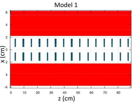
3.4 Photon collimator Model 1. . . 70
3.5 Photon collimator Model 2. . . 70
3.6 Polarisation (red) and number of photons transmitted (blue) as a func-tion of collimator aperture. The number of photons transmitted is nor-malised to the uncollimated beam. Analytical results (circles) are com-pared with Fluka simulation (crosses). . . 72
3.7 Intensity of radiation from the ILC helical undulator, as a function of normalised frequency. Red: uncollimated. Blue: collimated. . . 73
3.8 Polarisation of radiation from the ILC helical undulator, as a function of normalised frequency. Red: uncollimated. Blue: collimated. . . 73
3.9 Positron energy distribution after target. Top: no photon collimation. Bottom: 1 mm radius photon collimation. . . 76
3.10 Positron polarisation distribution after target. Top: no photon collima-tion. Bottom: 1 mm radius photon collimacollima-tion. . . 77
3.11 Positron distribution as a function of horizontal position. Top: no pho-ton collimation. Bottom: 1 mm radius phopho-ton collimation. . . 78
3.12 Positron distribution as a function of angle with respect to the undu-lator axis. Top: no photon collimation. Bottom: 1 mm radius photon collimation. . . 79
3.13 Positron phase space distribution after the target. Top: no photon col-limation. Bottom: 1 mm radius photon colcol-limation. . . 81
3.15 FLUKAGUI visualisation showing the energy deposititon per unit vol-ume per primary photon in the Model 1 collimator, using a 10 MeV incident photon beam. The plot has been projected onto thex−z plane (left) and x−y plane (right), where z is the direction of the incident photons. . . 84
3.16 FLUKAGUI visualisation showing the energy deposititon per unit vol-ume per primary photon in the Model 2 collimator, using a 10 MeV incident photon beam. . . 84
3.17 Temperature rise in spoilers and absorbers as a function of collimator aperture in Model 1. Also shown is the fraction of primary photons transmitted. . . 87
3.18 Temperature rise in spoilers and absorbers as a function of collimator aperture in Model 2. Also shown is the fraction of primary photons transmitted. . . 88
3.19 Equivalent dose rate for Model 1 (top) and Model 2 (bottom) when ap-plying various photon collimator apertures after operating for 180 days. The equivalent dose rates are shown immediately after operation (blue), after one hour of cooling (red) and after one day of cooling (green). . . . 89
3.20 Residual particle distribution in Model 1 (top) and Model 2 (bottom) with 3 mm aperture, following an operational period of 180 days. . . 90
3.21 Spoiler activation in Model 1 collimator, following an operational period of 180 days. The spoiler activation is shown immediately after operation (blue), after one hour of cooling (red) and after one day of cooling (green). 90
3.22 Model 2 activation in the graphite spoiler (top) and tungsten absorber (bottom) with various photon collimator apertures after operating for 180 days. The activation is shown immediately after operation (blue), after one hour of cooling (red) and after one day of cooling (green). . . . 91
3.23 Positron yield as a function of target thickness. . . 94
3.24 Energy deposition in target, adiabatic matching device and RF as a function of target thickness. . . 95
3.26 Positron energy spread immediately after the target, using ILC baseline parameters. . . 98
3.27 Positron transverse phase space immediately after the target, using ILC baseline parameters. . . 99
3.28 Trajectory of a particle with energy 5 MeV in the nominal AMD field and part of the constant solenoid field in the RF section. . . 101
3.29 Projection of the trajectory in Fig. 3.28onto thex−y plane. . . 101
3.30 Transfer efficiency as a function of initial magnetic field and taper pa-rameter in the AMD, using ILC baseline papa-rameters. . . 102
3.31 The number of positrons lost as a function as longitudinal position in the AMD, for a low field case. . . 103
3.32 Transfer efficiency as a function of magnetic field and aperture radius in the matching device. Standard ILC undulator-based positron source parameters have been assumed. . . 104
3.33 The positron transfer efficiency as a function of gap distance from target to entrance of the matching device. . . 105
4.1 Positron yield (per 100 m of undulator) and polarisation as functions of electron beam energy from 100 GeV up to 700 GeV, with ILC undulator parameters. . . 115
4.2 Yield per 100 m of undulator as a function of undulator period (deflection parameter 0.92), with 150 GeV electron beam energy (blue) and 250 GeV electron beam energy (red). The ILC damping ring acceptance is applied.116
4.3 Positron yield and polarisation from 100 m of undulator (deflection pa-rameter 0.92, and period 11.5 mm) as a function of electron beam energy. ILC damping ring acceptance is applied. . . 119
4.4 Positron yield and polarisation from 100 m of undulator (deflection pa-rameter 0.92, and period 11.5 mm) as a function of electron beam energy. CLIC predamping ring acceptance is applied. . . 119
4.5 Positron yield and polarisation as functions of photon collimator aper-ture, for CLIC Stage 1 parameters shown in Table4.2. . . 123
4.7 Positron yield as a function of target thickness in CLIC Stage 1. . . 126
4.8 Transfer efficiency in an AMD for CLIC Stage 1 (250 GeV electron beam energy in the undulator) as a function of initial magnetic field strength and taper parameter. . . 128
4.9 Transfer efficiency in an AMD for CLIC Stage 1 (250 GeV electron beam energy in the undulator) as a function of initial magnetic field strength and aperture radius. . . 128
4.10 Positron transfer efficiency in an AMD as a function of the size of the gap from the target to the entrance of the matching device, using CLIC Stage 1 parameters (250 GeV electron beam in the undulator). . . 129
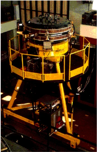
5.1 Target wheel experiment at Daresbury Laboratory, before installation of the safety cage. . . 135
5.2 Target wheel experiment at Daresbury Laboratory, enclosed in the safety cage. . . 136
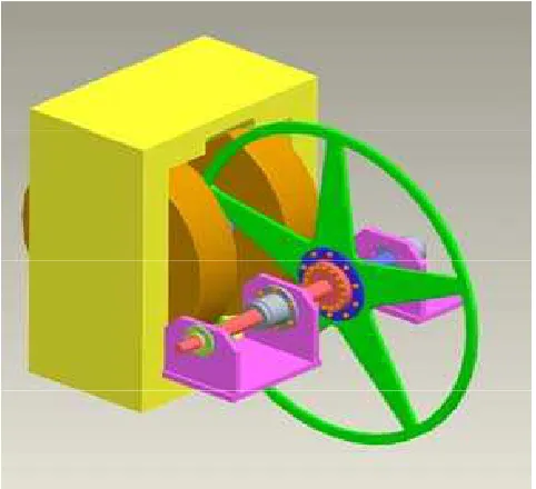
5.3 View of the target wheel at full immersion in the field of the magnet. . . 137
5.4 Field mapping obtained with Hall probe attached to the wheel rim. There is a constant current in the coils of the magnet, but the position of the magnet is varied to provide different immersion depths (correspond-ing to the different colour lines) of the target wheel. . . 138
5.5 Field mapping obtained with Hall probe attached to the wheel rim. The immersion depth is constant, but different currents (corresponding to the different colour lines) in the coils of the magnet are used. . . 138
5.6 The magnetic field strength as a function of the angle around target rim from an arbitrary zero position. The measured values are shown in blue; the air-core model is shown in red dashes, and the steel-core model is shown in green dots. . . 139
5.7 Simplified model of the target wheel moving in a magnetic field, allowing analytical calculation of the eddy currents and the resulting forces. . . . 141
5.10 Data from torque transducer channel Torque 1 (top) showing the target wheel rotating with nominal speed set at 33 rpm; then stopping for a few seconds; and then finally restarting and accelerating to a speed of 15 rpm. The bottom plot shows simultaneous data from the torque transducer Speed channel. . . 147
5.11 Data from torque transducer showing the target wheel accelerating from rest to a speed of 198 rpm; maintaining this speed for about 20 seconds; and then finally decelerating to rest. The top plot shows the torque; the bottom plot shows the speed. . . 148
5.12 Data from torque transducer showing the torque as the target wheel is accelerated from rest to a speed of 174 rpm; maintained at this speed for about 18 seconds; and then finally decelerated to rest. . . 150
5.13 Torque as a function of rotation speed for different immersion depths and magnetic field strengths. Red, green and blue lines show immersion depths 50.25 mm, 30.25 mm and 20.25 mm, respectively. Solid, dashed, and dot-dashed lines show magnet currents 100 A (1.44 T peak field), 50 A (0.9 T) and 27.275 A (0.485 T) respectively. . . 150
5.14 Comparison between experimentally measured torque (solid line), an-alytical estimate (red dots) and Opera simulation (blue dots), for the prototype target wheel immersed at a depth of 50.25 mm in a magnetic field with peak value 0.485 T. . . 152
5.15 As Fig. 5.14, but with the rim thickness increased by 50% to 45 mm in the analytical and Opera simulation models, to account for the effect of the spokes. . . 152
5.16 Equipment for titanium alloy material thermal test and thermal camera calibration. . . 153
5.17 Results from thermal camera calibration measurements. We increase the heater temperature from 0 to 200 as shown x-axis. The blue dots are the temperature reading from thermometer and red dots are the reading from thermal camera. . . 154
1.1 AdA parameters. . . 3
1.2 BEPC and BEPC-II parameters. . . 6
1.3 Global accelerator paramters for ILC. . . 17
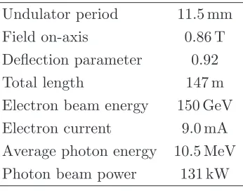
1.4 Undulator parameters for ILC. . . 21
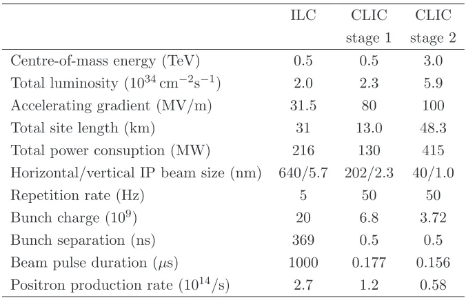
1.5 ILC and CLIC main parameters. . . 25
2.1 Theoretical cascade shower longitudinal and transverse containment in titanium. . . 47
2.2 FLUKA results of energy deposition in Region 1 and Region 2 in the longitudinal direction. . . 47
2.3 FLUKA results of energy deposition in Region 3 and Region 4 in the transverse direction. . . 48
3.1 ILC helical undulator parameters. . . 66
3.2 Effect of collimation on photon and positron beams, with fixed undu-lator, target and matching device parameters. Note that the positron yield is defined as the number of positrons produced per electron in the undulator. . . 75
3.3 Transfer efficiency, photon polarisation and energy deposition in different sections of the two collimator models, for different collimator apertures. The percentage in brackets following the total energy deposited gives the total energy deposited in the collimator as a percentage of the total energy in the incident photon beam. . . 83
4.1 Nominal acceptance specifications for ILC damping rings and CLIC pre-damping ring. . . 118
Introduction: Positron Sources
for Accelerators
1.1
Background: Particle Accelerators
Why do we need to build accelerators? Simply, an accelerator is an instrument for re-searching and knowing the microcosmic world. What is the composition of our bound-less universe? In all ages, people keep thinking about and exploring this question. An-cient philosophers can only deduce the answer based on the natural phenomena which they can feel they can see. For instance, the Greek philosopher Aristotle believed that all objects in the world consisted of four fundamental elements: earth, water, fire and air. China also had that kind of description, but instead of four they believed there were five fundamental elements, with gold as the extra one. Human society evolved over thousands of years to arrive at modern life. Along with technological develop-ments, people started to use more reliable methods – experiments – to validate their thinking. Particle accelerators are a bit like extremely powerful microscopes. They use high voltages to accelerate particles to high energies so that their wavelengths get smaller. An accelerator is a device that produces beams of particles, with controllable:
1. intensity (number of particles/unit time);
2. energy;
3. energy spread;
5. angular spread.
1.2
Accelerator Overview
Since the 1920’s high-energy accelerators have played a more and more important role in the research of fundamental particles and their interactions [1]. There are now several thousands of particle accelerators in the world. They are spread across many different fields such as industry, medicine and chemistry. But there are still also accelerators that are built in laboratories dedicated to academic research. For that purpose, the most advanced device is the collider, which accelerates two beams of particles to high energy and then lets them impact against each other. By observing and analysing the results of the collision, scientists find new particles and understand new phenomena [2]. In order to achieve higher energies, these machines have become progressively larger and more complex over time as shown in Fig. 1.1 [3]. There are several kinds of colliders, which may be classified according to the beams of particles they collide, such as proton-proton, proton-antiproton, electron-positron, etc. In this thesis, we will focus on electron-positron linear colliders. In the following sections of this chapter, some examples of electron-positron colliders over the past 50 years are briefly described, starting with the world’s first electron-positron collider – AdA [4] – and moving on to the electron-positron collider in China (the Beijing Electron-Positron Collider, BEPC [5]), the world’s largest electron positron collider, LEP and the first (also the only) linear collider the SLAC Linear Collider – SLC.
1.2.1 The First Electron-Positron Collider – AdA
Figure 1.1: Centre of mass energies in colliders, history and future prospect. Full symbol: past and present project. Empty symbols: future. Blue: leptons, Red: hadrons, Green: leptons-hadrons.
Table 1.1: AdA parameters.
Maximum c.o.m. energy 0.5 GeV
Radius 65 cm
Status Active from 1962 to 1965
to synchrotron radiation emission from the stored particles. Four years later, Frascati gave the first measurable luminosity value of 1025cm−2sec−1, which demonstrated the feasibility of the technology. In fact, after Anderson’s discovery of the positron, this was the first time positrons had been used in collider. The method of producing the positron beam in AdA became known as a “conventional” positron source. First of all, an electron beam struck an external target to produce bremsstrahlung gamma rays that entered the collider ring; the gamma rays then struck a metallic target (a thin tantalum sheet) that converted the gamma rays to electron-positron pairs.
revolutionised the use of accelerators in high-energy physics. It led to a rapid growth in the interest and development of electron-positron colliders, with more ambitious parameters, which in turn led to further research about positron sources.
1.2.2 The Chinese Electron-Positron Collider BEPC
The Beijing Electron-Positron Collider (BEPC) is a high energy accelerator designed for both high energy physics experiments and synchrotron radiation applications. It was proposed and designed in 1982, and was the first high energy particle accelerator to be built in China [6]. There are four main parts in the machine, including a 1.4 GeV electron and positron linac, a 2.2-2.8 GeV storage ring, a magnetic spectrometer for the high energy physics experiments, and synchrotron radiation facilities. Electrons are generated by an electron gun and then injected into the linac which is 202 m long. When the electron beam is accelerated to an energy of 150 MeV, the beam strikes a 10 mm tungsten target to create electromagnetic cascade showers. Electrons, positrons and photons are generated and are emitted from the target. The positrons are focused and captured, and accelerated to higher energy, to produce the positron beam for later collision. After the linac, there is a storage ring with circumference 240.4 m. The shape of the ring consists of two long straight sections of 27.4 m and two approximately semi-circular arcs. There is an interaction point in the middle of one long straight section. When the electrons and positrons are injected into the ring, the beam is accumulated until we obtain sufficient numbers of particle, and then the energy is ramped. The electron and positron beams are accelerated to the operating energy. Finally, the magnetic fields are maintained at constant levels, and the beams start to collide. The BEPC storage ring is refilled with electron and positron beams every 4–6 hours.
BEPC-II is an upgrade project of BEPC, and achieved its first collisions in 2008. There are two storage rings in the tunnel, so that electron and positron beams stay in their own ring. The luminosity that can be achieved is two orders of magnitude higher than the BEPC, up to 1033cm−2s−1. A comparison between the BEPC and BEPC-II parameters is shown in Table 1.2.
Table 1.2: BEPC and BEPC-II parameters.
BEPC-II BEPC
Energy (GeV) 1.0 – 2.1 1.0 – 2.5
circumference (m) 237.5 240.4
β∗
x/βy∗ (cm) 100/1.5 120/5
Number of bunches (Nb) 93 1
Beam intensity (E = 1.89 GeV) 2×910 2×35 Luminosity (E= 1.89 GeV) (1033cm−2s−1) 100 1
conventional source [7]. Electrons are accelerated to 240 MeV (140 MeV for BEPC) and strike a 10 mm diameter, 8 mm thick copper-plated, disc-shaped tungsten target. The target can be moved in and out of the beam line easily with the help of an actuation system. The positrons generated by pair-production will have a large divergence angle which needs to be focused to a reasonable size ready to be used in the later accelerat-ing section. In BEPC-II, there is a flux concentrator providaccelerat-ing a longitudinal magnetic field for this job. The flux concentrator is a device that has a 12-turn 10 mm long cop-per coil with a cylindrical outside radius of 53 mm and a conical inside radius growing from 3.5 mm to 26 mm. This device helps to match the phase space distribution of the positron beam from the target to the linac as explained in Chapter 2. The new BEPC-II positron source has been designed and fabricated since 2002, and has been shown to be a successful design.
1.2.3 The Large Electron-Positron Collider, LEP
achieved its target to produce sufficiently intense positron beams for LEP to reach its luminosity goals. The main purpose of LEP was for precision studies of both the Z and W bosons and for the search for new particles. In order to achieve the goal, the energy and luminosity of the machine were key parameters. From 1994 to 2000, by the hard work of many scientists, the energy and luminosity of LEP was improved significantly. In 1999, LEP reached its peak luminosity of just over 1032cm−2s−1[9], with an average daily integrated luminosity of close to 1.4 pb−1. In 2000 the beam energy achieved a
record high of 104.3 GeV. However, the luminosity was lower than the value of 1999 as a trade-off with the energy. The reduction is mainly due to the lower beam currents, shorter fills and larger horizontal beam sizes.
1.2.4 The SLAC Linear Collider, SLC
The Stanford Linear Collider (SLC) began construction in 1983 and was completed in 1989. Initially, the SLC was constructed as a prototype to demonstrate the feasibility of a high energy electron-positron linear collider. The SLC was the world’s first and only linear collider [10]. A schematic of the facility is shown in Fig. 1.3. SLC accelerated electrons and positrons to about 50 GeV using the same, two-mile long linac. In each machine pulse, the source generated two bunches of polarised electrons. The first one was used for collision, and the second one was used to generate a positron bunch. The electron and positron bunches were first injected into damping rings, to reduce the bunch dimensions to sizes suitable for generating luminosity. When the electron and positron bunches were extracted from the damping rings, they were then injected into the linac, which accelerated the particles to 46.6 GeV. At the end of the linac, the electron and positron bunches were separated into two long curving arcs. In the arcs, the particles lost about 1 GeV energy, because of synchrotron radiation. The electron and positron bunches then collided head-on at the interaction point (IP) with a centre-of-mass energy of 91.2 GeV. The bunches were dumped after collision.
Figure 1.3: Schematic view of the SLAC Linear Collider.
a thick, high-Z material target to generate positrons by cascade shower. Due to the large divergence angle of the positrons coming from the target, a flux concentrator was used, which helped to improve the capture efficiency, and so increased the overall positron yield. The SLC positron source has been discussed in detail in references [11] and [12]. As the first and only linear collider in the world, SLC provided essential experience for the design of a next generation electron-positron linear collider. Future linear collider projects presently under study will be introduced in the following sections.
1.3
From Circular to Linear Colliders
electromag-netic and weak nuclear forces, detector backgrounds are much higher in proton-proton colliders than in positron colliders. For precision measurements using electron-positron collisions, a linear collider is the best answer [13][14]. There are two future linear colliders that have been proposed: these are the International Linear Collider (ILC), and the Compact Linear Collider (CLIC), which we will introduce in later sec-tions.
In 2010, one of the most exciting events in scientific research will be operation of the Large Hadron Collider (LHC) in CERN, Geneva. The advantage of LHC is its high collision energy of 7 TeV protons, but as already mentioned, the detector back-grounds in LHC will be much higher than in an electron-positron collider, because of the strong interactions of the hadrons, and their sub-structure. Hence, in general, LHC will be a discovery machine for new physical phenomena, but not sufficient for preci-sion measurements and research. Therefore, a precipreci-sion machine is needed that can be complementary to the LHC.
An electron-positron collider will be ideal, because the particles have no sub-structure, and interact only through the electromagnetic and weak interactions. However, if we want to accelerate electrons or positrons to energies of the order of 1 TeV in a storage ring, there will be significant power losses because of synchrotron radiation. When charged particles circulate in storage rings, they lose energy at a rate proportional to the fourth power of the beam energy, and inversely proportional to the square of the radius of the trajectory:
Ps=
e2c
6πε0 1 (m0c2)4
E4
R2, (1.1)
where Ps is the radiated power during transverse acceleration, E is the energy of the
particle,ethe charge on the particle,m0 the rest mass of the particle,Ris the bending radius of the particle orbit, c is the speed of light, and ε0 is the permittivity of free space.
For particles of a given energy and charge, the radiated power varies inversely with the fourth power of the rest mass. Comparing the power radiation from an electron (mec2=0.511 MeV) with that from a proton of the same energy (mpc2=938.19 MeV)
gives:
Ps,e
Ps,p
=
mpc2
mec2
4
≈1.13×10¹³. (1.2)
of magnitude larger for electron than for protons: thus a proton-proton machine such as the LHC which is circular with TeV energy is practicable, but a circular electron-positron machine operating at similar energy is not. In order to avoid the loss of large amounts of energy by synchrotron radiation that happens when high energy electrons or positrons follow a circular trajectory, the next generation electron-positron collider must be linear. However, to keep costs realistic, the size of the linear collider needs to be kept reasonable. In general, the accelerating gradient of superconducting RF cavities has a fundamental limit at about 60 MV/m. With normal conducting RF structures, higher gradients are achievable, but the technology is not trivial and still under development. A linear collider will need high gradient RF cavities, since the beam needs to be accelerated to high energy in a limited distance. There are two linear colliders, based on different technologies, that have been proposed and are being developed in parallel. The ILC will use superconducting technology to accelerate the electron and positron beams to 250 GeV, to achieve collisions at centre-of-mass energy of 500 GeV. CLIC is based on two beam acceleration to reach centre-of-mass energy of 3 TeV. In later sections, further details about these two machines will be introduced.
1.4
Positron Sources for Linear Colliders
1.4.1 Conventional Source
A conventional positron source is based on the use of high energy electrons striking a high Z material target to generate electromagnetic cascade showers (thick target) or pairs of electron and positrons (thin target) [16]. In general, the electron beam will have an energy of a few GeV; when the electrons impinge onto the target, the electrons will lose energy by radiation and collision with the atoms. In this process, the energy lost through radiation (bremsstrahlung) is distributed among photons which interact with the Coulomb fields of the nuclei in the target material, resulting in production of electron-positron pairs. These processes continue in turn, until the remaining particles have energy too low for further pair production. Electrons and photons then lose energy via scattering until they are eventually absorbed by atoms. The energy lost by collision is deposited in the target as heat. The energy deposition and heating is a major concern in the use of conventional positron sources. Another concern is the emittance of the positron beam since in the process of propagation through the material of the target, there will be multiple scattering, resulting in a large angular distribution for the positrons. There are several designs that have been used in previous accelerators, such as classical thick amorphous disk targets. In order to limit the transverse size increase caused by multiple scattering, and also to allow the low energy positrons to leave the target instead of being absorbed, a design based on a wire target has been proposed. Another popular idea is to use separate targets for photon production and electron-positron pair production. Basically, there are two targets: the first one will be used as a radiator to produce the photons and the other target will be used as a converter for the materialization of the photons into electron and positron pairs. The advantage of using separate targets is that it is possible to avoid excessive thermal heating using a crystal in channelling conditions to deliver an intense photon beam to a thin converter.
The conventional positron source is a classic design that has been used in many accelerators. The advantages of this design are that:
1. it is a mature and reliable, proven concept;
2. it operates independently of the main electron source;
However, at the same time this scheme also has some limitations that need to be considered:
1. multiple scattering will affect the positron angular distribution which leads to a large emittance;
2. high energy electrons and ionization in the target cause energy deposition and heating problems;
3. it is very difficult to produce polarised positron beams.
1.4.2 Undulator-Based Positron Source
The undulator-based positron source is the baseline design for the International Linear Collider. The advantages of an undulator-based positron source are that:
1. a prototype has been built and tested;
2. it is possible to produce a sufficiently intense positron beam;
3. a helical undulator can be used to generate polarised positrons;
4. a thin target can be used, which results in lower energy deposition compared with a conventional source.
As always, this scheme is not perfect, there are disadvantages as well:
1. the source is dependent on the electron beam, which complicates the timing scheme of a linear collider;
2. large amounts of specialised infrastructure are needed, which limits the applica-tion;
3. the main electron beam will gain additional energy spread as it passes through the undulator;
4. if collision energies are needed that are below the energy at which the electron beam must pass through the undulator, then the electron beam must be deceler-ated before collision.
1.4.3 Compton Source
produced is very small, which means that the number of positrons generated will be very small. The solution is that for this scheme, the positrons are produced slowly and must be accumulated in a damping ring, which is one of the biggest challenges. However, a lot of scientists worldwide are working on this scheme, trying to solve existing problems such as:
1. production of high-intensity laser beam;
2. achieving the necessary collision efficiency and duration;
3. re-use of electron and photon beams;
4. design of a damping ring with sufficient acceptance to allow injection of newly-produced positrons without loss of stored positrons.
But it is worth tackling the challenges, since the mature Compton scheme will be very beneficial for several reasons:
1. it will be possible to generate polarised positrons;
2. the system is completely independent of the main electron beam;
3. a relatively low energy electron beam is required;
4. the scheme could be used in a wide range of potential applications.
1.4.4 Other Positron Source Schemes
positron sources described above will appear in the near future, with applications to particular projects that will maximise particular advantages.
1.5
Linear Collider Projects and Their Positron Sources
The International Linear Collider (ILC) is a proposed high energy electron-positron linear collider with a baseline centre-of-mass energy of 500 GeV, supporting a later upgrade to 1 TeV, and a baseline luminosity of 2×1034cm−2s−1 [20]. The ILC is important for future precision physics measurements, complementary to experiments at LHC. It will allow the acceleration of electrons and positrons, which have no observed sub-structure and no interaction through the strong nuclear force; so it will be easier to analyse accurately the collision data at ILC than at the LHC, which is more of a discovery machine and will (we hope) find the Higgs bosons if it exists. Another feature of the proposed ILC is the use of polarised beams. This is important because polarised electron and positron beams lead to a much higher precision for probing the properties of new particles. Furthermore, suitable combinations of the electron and positron polarisation can be used to enhance signal rates of interesting processes and suppress unwanted background. Hence an increase in the ratio of signal/background combined with high luminosity will allow promising future research.
The Compact Linear Collider (CLIC) is an advanced future electron-positron col-lider to exploit the LHC’s discoveries in a new high energy frontier, which is beyond the capabilities of today’s accelerators [21]. CLIC is an electron-positron machine aiming to operate at a centre-of-mass energy range from 0.5 TeV to 3 TeV. Both ILC and CLIC are electron-positron linear colliders designed for precision physics measurements. Al-though the two machines are based on very different acceleration technologies, there are sufficient similarities that it is worth considering whether some of the features of the more mature ILC design can be adapted and re-optimised for use in CLIC.
the ILC undulator-based scheme to discuss the key components, such as the helical undulator, photon collimator, target, and matching device. After the ILC chapter, we will consider the possibility of implementing an undulator-based positron source for CLIC. The optimisation in different scenarios of operating energy and upgrade options will be discussed. Finally, there will be a conclusion about the possibility of using an undulator-based positron source in CLIC, and its advantages and weaknesses compared to the present baseline scheme.
1.5.1 International Linear Collider
The ILC is a high-energy collider designed for precision studies of the Higgs boson and other phenomena yet to be observed, such as super-symmetry. Fig. 1.4 depicts schematically the layout of the ILC baseline configuration [20]. The ILC is approxi-mately 31 km long. Electrons and positrons will be collided at centre-of-mass energies of 500 GeV (with the possibility to upgrade to 1 TeV). Electrons and positrons are ac-celerated in separate linacs. At the interaction point, particle bunches containing of order 1010 particles are focused to a width of 650 nm and a height of 5 nm, and collide at a rate of 14,000 times per second. The global parameters of the ILC are given in Table1.3.
Figure 1.4: Schematic view of the International Linear Collider baseline configuration.
Table 1.3: Global accelerator paramters for ILC.
Centre-of-mass energy 500 GeV Peak luminosity 2×1034cm−2s−1
Repetition rate 5 Hz
Linac cavity gradient 31.5 MV/m Beam pulse length 1.0 ms Beam current in pulse 9.0 mA Beam size at IP 640 nm×5.7 nm
fill time, which can itself reduce the power efficiency. To maintain efficient operation, the RF pulse length should be long compared to the fill time: in ILC, the beam pulse has a total length of 1 ms. The long fill time also limits the average beam current. If the beam current is too high, then the beam will draw energy from the cavities more quickly than it can be replaced. In ILC, the average beam current is 9 mA. The ILC parameters have been chosen to maximise operational performance while minimising construction and operating costs. However, the RF parameters are still ambitious for a machine on the scale of ILC. There are several test facilities all over the world, in-cluding at Fermilab in the USA and at KEK in Japan. There has been a significant improvement in the technology over the past few years, but there are still challenges to achieve the desired results. In particular, it is difficult to produce on a large scale cavities that can reliably achieve the accelerating gradient required in ILC. Reducing the gradient specification would mean that a longer linac would be required for the same collision energy, and this would increase the cost of the machine.
and energy compression on the way. The LTR will bend the 5 GeV polarized electron beam through an arc. If the first bend of the LTR is turned off, the 5 GeV beam is sent to a beam dump which can be used for machine protection or for tuning.
Following the LTR is a Damping Ring with a circumference of 6.7 km. The Damp-ing RDamp-ing performs several critical functions, principally acceptDamp-ing electron and positron beams with large transverse and longitudinal emittances and producing the low-emittance beams required for luminosity production. Furthermore, it damps incoming beam jitter to provide stable beams for later use. After being ejected from the Damping Ring, the bunch train will go through the Ring-to-Main Linac (RTML) beam line. The electron beam will be accelerated to 15.0 GeV before injection into the main linac. Also short bunches are required for collision, so the RTML will compress the beam from 9 mm in the Damping Ring bunch length to 0.3 mm, required at the Interaction Point (IP) to minimise the hour-glass effect. At the same time, the RTML can collimate any beam halo generated in the Damping Ring and rotate the spin polarisation vector from the vertical to any arbitrary angle required at the IP. In the 11 km linac, the electron beam is accelerated to a final energy of 250 GeV.
The luminosity of a linear collider is given by:
L= nbN 2f
rep
4πσxσy ·
HD, (1.3)
wherenb is the number of bunches in a bunch train,N is the number of particles in a
single bunch,frep is the machine pulse repetition rate,σx andσy are the horizontal and
vertical beam sizes at the IP, andHD is the ‘enhancement factor’ (∼1.5) that accounts
for the mutual focusing effects of the colliding bunches. The number of bunches, par-ticles per bunch, and pulse repetition frequency are all limited by the RF technology in the linacs. Therefore, to maximise the luminosity, the transverse beam sizes must be made as small as possible. To meet the luminosity goal, the Beam Delivery System (BDS) focuses the beam to a spot size of 640 nm horizontally and 5 nm vertically at the interaction point. The BDS also protects the beam line and detectors, minimises background in the detectors by collimating the large amplitude particles, and measures and monitors the beam before and after collisions. Finally, after collision each beam will go through an extraction line to a beam dump.
emit multi-MeV photons. The generated gamma rays will be collimated by a photon collimator which can help to protect the target station and improve polarisation. The collimated photons will then be converted to electron-positron pairs in a target. Fig.1.5
shows the major elements of the positron source [22].
Figure 1.5: Schematic view of the ILC undulator-based positron source.
Longitudinally polarised positron beams can be produced from a beam of circularly polarised photons, which are themselves produced by passing the main high-energy electron beam through a helical undulator. A helical undulator is a device that has a ‘rotating’ magnetic field (as a function of distance along the undulator) in which electrons will move in a spiral trajectory. The motion of the electrons in the magnetic field of the undulator causes them to emit a stream of photons. Circularly polarised photons are used to generate longitudinally polarised positrons in a conversion target. The principle of the device is shown in the Fig.1.6 [23].
Figure 1.6: Principle of polarised positron production from high-energy electrons in a
helical undulator.
experiment (E166, performed at SLAC [24]) has demonstrated the successful production of polarised positrons using this technique. A prototype for a helical undulator for the ILC undulator-based positron source is shown in Fig.1.7.
Figure 1.7: Top: Double helix winding with opposite currents generate a rotating
mag-netic field as a function of longitudinal distance along the undulator axis. Bottom: Proto-type of a helical undulator for the ILC positron source.
In the ILC, it is planned to use superconducting undulator technology to achieve a high field with a short period. Because a helical undulator provides a more efficient way of generating photons than a planar undulator, the overall length can be shorter for the same quantity of photons. One additional advantage of the undulator-based source is that the heat load on the target is less than that of the conventional source, so it is suitable for production of high intensity beams. The parameters of the baseline ILC helical undulator are shown in Table 1.4.
re-Table 1.4: Undulator parameters for ILC.
Undulator period 11.5 mm
Deflection parameter 0.92
Undulator type Helical
Undulator length 200 m
Field on-axis 0.86 T
Beam aperture 5.85 mm
Electron beam energy 150 GeV
Electron current 9.0 mA
Photon energy(1st harmonic cutoff) 10.06 MeV
Photon beam power 131 kW
duces the beam intensity. So we cannot just use the first harmonic of the photon beam, which has the highest polarisation. All in all, there must be some compromise between polarisation and quantity of positrons. The photon collimator provides the means to adjust the balance between polarisation and beam intensity. There are different design concepts for the photon collimator already proposed by DESY and Cornell. In the next chapter we will discuss further the photon collimator, including various geometries and performance simulations.
After collimation, the photons hit a thin target producing an electromagnetic shower to generate electron and positron pairs. The target will be discussed in more detail in the following chapters. The distance from the centre of the undulator to the target is about 500 meters. The photon beam has a transverse size of∼1 mm rms and deposits
diameter) offsets radiation damage.
Figure 1.8: Design for the rotating target for the ILC positron source.
The energies of particles coming out of the target are in the range 3–55 MeV. The target is followed by an Optical Matching Device (OMD) which is used to match the beam phase space from the target into the capture L-band RF. The capture RF raises the beam energy to 125 MeV; RF cavities are located inside 0.5 T solenoids that focus the beam. Because the target and associated equipment become highly activated during operation, there is a remote-handling system to replace the target in the case of target failure. Following the capture section, the positron beam will be accelerated from 125 MeV to 400 MeV in a normal-conduction L-Band RF, again embedded in a solenoid field of 0.5 T. From this point, the positron beam will pass through systems identical to those used for the electron beam, including the LTR, the Damping Ring, the RTML, the main linac and the BDS.
1.5.2 Compact Linear Collider
accelerating gradient that can be achieved using a superconducting cavity is limited by the fact that the strong magnetic fields generated inside the cavities will quench the superconducting material if the gradient gets too high. A higher energy can be achieved by using longer linacs, but this will increase the cost of the machine. Therefore, an al-ternative accelerating technology is required to achieve centre-of-mass collision energies of more than 1 TeV.
a conventional source, a source based on Compton back-scattering, and an undulator scheme. Some characteristics that must be taken into consideration for the choice of the source include the achievable production rate and polarisation. In later sections, the undulator scheme will be considered in detail, as an option for the CLIC positron source.
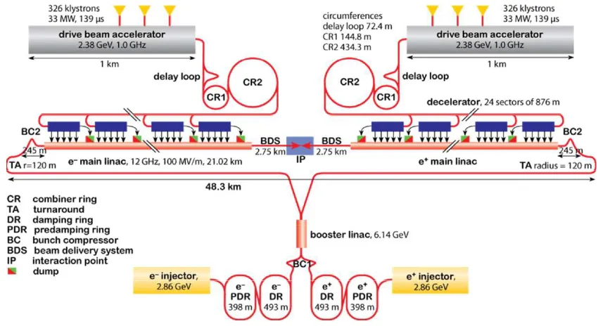
Figure 1.9: Schematic view of the Compact Linear Collider (CLIC).
Table 1.5 shows some of the main parameters of ILC and two operational stages of CLIC. Although the machines have a number of things in common, the different RF technology used to accelerate the beam in CLIC compared to ILC makes each machine unique. ILC uses a long RF pulse, with relatively low average beam current in the linacs. CLIC uses a short pulse with high current. By focusing the beams more strongly at the IP, CLIC achieves a similar luminosity to ILC with a smaller number of particles. ILC will require 2.7×10¹⁴ positrons per second, while CLIC will require 1.2×10¹⁴ (stage 1, 0.5 TeV c.o.m.) or 0.58×10¹⁴ (stage 2, 3 TeV c.o.m.). Although CLIC requires a lower positron production rate than ILC, the shorter pulse and higher repetition rate means that the positron source will not necessarily be any easier.
Table 1.5: ILC and CLIC main parameters.
ILC CLIC CLIC
stage 1 stage 2 Centre-of-mass energy (TeV) 0.5 0.5 3.0 Total luminosity (1034cm−2s−1) 2.0 2.3 5.9 Accelerating gradient (MV/m) 31.5 80 100
Total site length (km) 31 13.0 48.3
Total power consuption (MW) 216 130 415 Horizontal/vertical IP beam size (nm) 640/5.7 202/2.3 40/1.0
Repetition rate (Hz) 5 50 50
Bunch charge (109) 20 6.8 3.72
Bunch separation (ns) 369 0.5 0.5
Beam pulse duration (µs) 1000 0.177 0.156 Positron production rate (1014/s) 2.7 1.2 0.58
for large numbers of positrons. This puts stress in particular on the conversion target, and design options need to be studied carefully, to make sure that the target can survive both the peak and the average power deposition.
The baseline option for the CLIC positron source is the Compton scheme. Although this design should be able to produce enough positrons, it is still a new scheme that needs a lot of research. Other designs that have been proposed include a modified conventional design using a hybrid target, and an undulator-based scheme similar to ILC. Each option has its own advantages and disadvantages [27], which we will now consider briefly.
accelerated. There are several disadvantages in this design. Although this type of positron source is relatively simple, low cost and independent from the electron source, there is no polarisation at all, and the thermal load on target is difficult to handle.
e
-e
-e
-e+
J e
J
crystal e+ amorphous
Figure 1.10: Schematic view of the hybrid target positron source.
Another more advanced proposal is the Compton source [18]. A laser beam collides with a high energy electron beam, from which the laser photons will gain energy. The back-scattered photon beam (now with short wavelength and higher energy) will strike a target to produce electron and positron pairs. This technology is not sufficiently mature for immediate implementation, although there is much research activity on its development. The advantages of the Compton source are that it is independent from the electron source, and it has the capability for producing a polarised positron beam.
of an undulator-based positron source is that the source uses the main electron beam as the driving beam, which means that a high energy electron beam is needed before positrons can be produced, and also leads to complications for the timing scheme.
1.6
Thesis Layout
In Chapter 2 the theoretical background on synchrotron radiation is reviewed. The relevant details of undulator radiation regarding the photon spectrum and angular distribution will be discussed. The theoretical results will be compared with simulation results. Also in this chapter, the components of the undulator-based positron source will be described. In addition, the timing issues (related, for example, to the damping rings) will briefly be discussed. This chapter will provide an understanding of the detailed properties of undulator radiation, and how an undulator-based positron source will work.
Chapter 3 will consider the ILC in more detail. The theory of the undulator-based positron source will be applied, using ILC parameters. Most components of the ILC positron source have previously been studied in some detail. However, although some proposals have been made for the ILC photon collimator design, these have not so far been thoroughly considered and compared. Therefore, the photon collimator will be discussed in detail in this chapter. By using realistic distributions for the photons generated by the undulator, the energy deposition and thermal issues for the photon collimator will be investigated. How the collimator affects the photon beam, and the positron production and polarisation, will be explained. The activation and secondary particle generation from the collimator will also be discussed. This chapter will provide a more detailed understanding of the ILC positron source, and of the photon collimator in particular. By comparing two of the proposed designs for the photon collimator, we can identify the right collimator to be used for the ILC baseline.
positron production, positron polarisation, and capture efficiency.
A key issue for the positron source is the energy deposition in the target. In Chapter 5, we will discuss the target wheel experiment which has been carried out at STFC Daresbury Laboratory. We will introduce the mechanical design of the prototype. Positron capture efficiency can be improved if the target is immersed in the magnetic field of the matching device. However, to handle the energy deposition, the target wheel must spin with a rim velocity of 100 m/s, and if this rotation takes place in the magnetic field, then large eddy currents can be induced. The goal of the target wheel experiment at Daresbury is to measure the effects of the eddy currents, and validate the models that predict their effects. In order to understand the eddy currents, we will approach the problem by developing a theoretical model. Since the problem is very complicated, we also run simulations using OPERA. The results from the theoretical models and simulations will be analysed and compared with experimental data.
Components of an
Undulator-Based Positron Source
In this chapter, we introduce each of the main components of an undulator-based positron source. Section 2.1 describes the principles of the helical undulator, and the properties of the radiation that it produces. Section2.2introduces the photon collima-tor, discussing issues such as energy deposition and activation. Section 2.3 describes the pair production target. Finally, Section 2.4 introduces the capture device that is used to match the phase space of the positrons from the target, to the entrance of the first accelerating section seen by the positron beam.
Our aims in this chapter are to outline the physical principles behind each of the components of an undulator-based positron source, and to understand general features and properties. We will give examples based on parameters relevant for ILC and CLIC where such examples are helpful; but detailed discussion of undulator-based positron sources for these machines will be left to later chapters.
2.1
Undulator
the strength of the field remains constant, while the direction “rotates” with distance along the undulator [17]. Helical undulators can be used to produce polarised beams of positrons. The degree of polarisation depends not just on the undulator, but also on the components downstream of the undulator.
As high energy (tens of GeV) electrons pass through an undulator, they emit syn-chrotron radiation. The synsyn-chrotron radiation can be collimated (if necessary) before impacting the pair production target. In this section, we focus on the properties of the radiation produced by the undulator, beginning with a general description of syn-chrotron radiation.
2.1.1 Synchrotron Radiation
Synchrotron radiation is the electromagnetic radiation emitted by relativistic charged particles when they undergo acceleration. Such radiation was first observed from a General Electric synchrotron in 1947 [28]. Synchrotron radiation is produced whenever a relativistic charged particle is bent in a magnetic field, and can cover a range of the electromagnetic spectrum from infrared, through visible light and ultraviolet light to x-rays.
As a consequence of synchrotron radiation, relativistic charged particles in a mag-netic field will lose energy. As accelerator technology has developed, the ability to add energy to charged particles has improved. Synchrotron radiation can be a severe lim-itation for high energy electron accelerators [29]. The power lost through synchrotron radiation varies as:
∆E∝ 1 ρ2m4
0
, (2.1)
To understand synchrotron radiation, two key effects are Lorentz contraction and relativistic Doppler shift [30]. For example, consider an electron that travels through an undulator (period λu) at (close to) the speed of light. In the moving frame, the
period of the undulator will be contracted by a factor of γ, and so the electron will emit the radiation with wavelength λu
γ. For the relativistic Doppler shift, in the case of
the particle travelling with the speed of light towards the observer, the frequency will change to:
f =γf′(1 +β), (2.2)
where the observer will see radiation at a frequency f, the source (electron) emits radiation at frequency f′ in its own rest frame, and β = v
c where v is the velocity of
the electron. If we convert the frequency of the radiation to the wavelength, we get:
λ= λ′
γ(1 +β) ≈
λ′
2γ. (2.3)
We see that the wavelength of radiation observed in the rest frame of the undulator isλu/2γ2. Modern accelerators readily achieve energies of a few GeV; for electrons, the
relativistic factorγ can be a few thousands. For an undulator with a period of order 0.1 m, the synchrotron radiation can have a wavelength of a few nanometres. A further important property of synchrotron radiation, is that the radiation is emitted into a narrow cone of opening angle 1/γ around the instantaneous direction of motion of the particle. For an undulator, interference effects lead to a further narrowing of the cone by a factor√N, whereN is the number of periods in the undulator. This means that undulators can be used in high energy accelerators to produce beams of very intense radiation with wavelengths of a few nanometres.
2.1.2 Electric and Magnetic Fields Around a Relativistic Charged Particle
The electromagnetic potentialsφandA~ around a charged, point-like particle are given by the Li´enard-Wiechert potentials [31]:
φ(t) = e 4πǫ0
" 1
r(1−~n·β~) #
ret
, (2.4)
~
A(t) = e 4πǫ0c
"
~ β r(1−~n·β~)
#
ret
, (2.5)
whereeis the charge on the particle,r is the distance from the position of the particle to the observation point, ~n is a unit vector from the position of the particle to the observation point, and β~ is the velocity of the particle divided by the speed of light. Note that the quantities inside the brackets [·]ret must be evaluated at a timet′, where:
t=t′+r(t′)
c , (2.6)
in order to find the correct values for the potentials at timet. For a relativistic particle moving directly towards the observer (~n ·β~ ≈ 1), there is an enhancement of the electromagnetic potentials; while the potentials are reduced for a particle moving away from the observer.
The electric and magnetic fields may be obtained from the potentials using the usual relations:
~
B = ∇ ×A,~ (2.7)
~
E = −∇φ−∂ ~A
∂t. (2.8)
For a particle on an arbitrary trajectory, application of the derivatives to Eqs. (2.4) and (2.5) is complicated, because r,~n andβ~ are all functions of time; andr and~n are additionally functions of position (of the observer). However, it is possible to perform the derivatives. The result for the electric field is [17]:
~ E = e
4πǫ0 "
(1−β2)(~n−β~)
r2(1−~n·β~)3 +
~n×((~n−β~)×β~˙)
cr(1−~n·β~)3 #
ret
, (2.9)
and for the magnetic field:
~ B = 1
Note that the second term on the right hand side of Eq. (2.9) depends on the acceleration of the particle β~˙. Also, this term varies with distance from the source as ∼1/r, whereas the first term varies as ∼ r2. This means that for an accelerating particle, at a sufficient distance from the particle, the fields are dominated by the second term in Eq. (2.9). The region where this second term does dominate the fields is known as thefar field orradiation region, and is the region we shall be concerned with.
It turns out to be convenient to work with the frequency spectrum of the fields, rather than the fields expressed as functions of time. The frequency spectrum of the electric field is given by the Fourier transform ofE~(t):
˜
E(ω) = √1
2π
Z ∞
−∞
~
E(t)eiωtdt. (2.11) Working in the radiation region, we can substitute for E~(t) from Eq. (2.9), and at the same time change the variable of integration fromt tot′ using Eq. (2.6). This gives:
˜
E(ω) = e 4π√2πǫ0
Z ∞
−∞
~n×((~n−β~)×β~˙)
cr(1−~n·β~)2 e
iω(t′+r
c)dt′. (2.12)
Let us assume that the observer is sufficiently far from the particle that~n is constant: this is consistent with working in the radiation region. Then, we can integrate Eq. (2.12) by parts to give:
˜
E(ω) = iωe 4π√2πǫ0cr
Z ∞
−∞
(~n×(~n×β~))eiω(t′+rc)dt′. (2.13)
2.1.3 Electromagnetic Radiation from a Relativistic Charged Particle
The energy flux (energy crossing unit area per unit time) in an electromagnetic field is given by the Poynting vectorS~ [32]:
~
S =E~ ×H~ = 1
µ0
~
E×B.~ (2.14)
Using Eq. (2.10) this becomes:
~
S(t) = ~n
µ0c E~(t)
2
. (2.15)
The total energy per unit area crossing the observation point is given by:
Z ∞ −∞ ~ S(t)
dt= 1
µ0c Z ∞ −∞ ~ E(t)
2
Using Parseval’s theorem [33], this becomes:
Z ∞
−∞
S~(t)
dt=
1
µ0c Z ∞
−∞
E˜(ω)
2
dω. (2.17)
From Eq. (2.15), we see that the energy flow is in the direction of~n, the unit vector from the source to the observer. Therefore, using dA = r2dΩ (where dA is an area element corresponding to solid angle elementdΩ centred on the particle), we can write the spectral energy distribution (energy crossing unit area per unit frequency) as:
d2W dω dΩ =
2r2 µ0c E˜(ω)
2
. (2.18)
Note the factor of 2, that comes from the fact that the electric field E~(t) is real, so ˜
E(−ω) = ˜E(ω). Including the factor 2 allows us to consider only positive frequencies in the spectral energy distribution. Finally, substituting from Eq. (2.13), we have:
d2W
dω dΩ =
ω2e2 16π3ǫ 0c Z ∞ −∞
(~n×(~n×β~))eiω(t′+rc)dt′ 2 . (2.19)
Eq. (2.19) is a general expression for the spectral energy distribution (energy per unit frequency range per unit solid angle) emitted by a relativistic charged particle in a magnetic field. ~n is a (constant) unit vector from the magnetic field to the observer. Note that the velocityβ~ of the particle is a function of the retarded timet′. Therefore,
the spectral energy distribution depends on the Fourier transform of the particle’s velocity as a function of time.
2.1.4 Undulator Radiation
The spectral energy distribution of synchrotron radiation from a particle with a given trajectory can be calculated from Eq. (2.19). There are a number of ‘standard’ systems (e.g. a dipole magnet) for which the integral in Eq. (2.19) can be performed. We are interested in the case of a helical undulator. In this case, the trajectory of an electron is a helix, with period equal to the period of the undulator, and amplitude depending on the strength of the magnetic field and the energy of the electron. The integral in Eq. (2.19) is quite complicated in this case, but it has been performed [34]. The result is:
d2W dω dΩ =
ω2e2K2
4π3ǫ 0cω20γ2
∞
X
n=1 "
J′2
n(x) +
γθ K − n x 2
Jn2(x) #
sin2hN πωω1 −ni
ω ω1 −n
Here,γ is the relativistic factor for a particle in the undulator, θ is the angle between the undulator axis and the observation point, and N is the number of periods in the undulator. Other quantities appearing in this expression are as follows:
K = λueB 2πmec2
, (2.21)
x = Kθ
γ ω ω0
, (2.22)
ω0 =
2πβ∗c
λu
, (2.23)
ω1 = ω0
1−β∗cosθ. (2.24)
λu is the undulator period, andB is the field strength. β∗ is the average velocity of a
particle in the longitudinal direction, divided by the speed of light. It is given by [34]:
β∗ =β
" 1− λu 2πρ 2# 1 2 =β " 1− K γ 2# 1 2 , (2.25)
whereρis the radius of the helical motion of a particle in the undulator. Note that ω0 is the circular frequency of the electron’s helical orbit. The physical significance ofω1 will become clear shortly. For now, we note that for ultrarelativistic particles (β ≈1) and for small angles θ,ω1 can be approximated by:
ω1≈
2γ2ω0
1 +K2+γ2θ2. (2.26)
Some interesting properties of the radiation spectrum can be seen by looking at the radiation on the undulator axis. That is, we take the limit θ → 0. In that case, Eq. (2.20) becomes:
d2W dω dΩ
θ=0 = ω
2e2K2 16π3ǫ
0cω02γ2
sin2hN πωω1 −1i
ω ω1 −1
2 . (2.27)
If the number of undulator periodsN is large, then the radiation spectrum has a single sharp peak at ω=ω1. For ultrarelativistic particles (i.e. β ≈1):
1 1−β∗ ≈
2γ2
1 +K2. (2.28)
So we can write (forθ= 0):
ω1≈ 2γ2