2018 2nd International Conference on Applied Mathematics, Modeling and Simulation (AMMS 2018) ISBN: 978-1-60595-580-3
An Automatic Annotation Algorithm for Deep Learning Image Datasets
Based on HOG Features
Fei YE
1and Xiao-guo ZHANG
1,*1
School of Instrument Science and engineering, Southeast University, Nanjing 210096, China
*Corresponding author
Keywords: Deep learning, Data annotation, HOG features, Image clustering, Deformable part models.
Abstract. Labeled data is crucial for deep learning model training, but it is mainly based on manual annotation. This paper proposes an automatic annotation algorithm for deep learning image datasets based on HOG features. The algorithm obtains the position information of the target based on the Gaussian mixture model, and automatically obtains the target category based on the Mean Shift algorithm of HOG feature. The labeled sample obtained in the above steps is used to train the Deformable Part Model to annotate more unlabeled image data. Experimental results show that this algorithm can quickly complete the automatic annotation of image datasets, reduce the cost of acquiring labeled datasets and greatly improve the effectiveness of acquiring labeled datasets in deep learning.
Introduction
Deep learning [1] is an important breakthrough in the field of artificial intelligence in the past decade. The quality of training data directly affects the quality of the model, which demonstrates the importance of data and features in the supervised learning network. Many researchers are faced with the problem that labeled data is limited and it is very difficult and expensive to obtain new labeled data. There are already some popular datasets annotation tools, such as LabelImg[2] and BBox-Label-Tool[3] and the video-based annotation tool Vatic, which rely on manual annotation. Lior Wolf proposes a method of labeling pictures using deep learning and Fisher vectors [4], but the annotations are descriptions of the pictures. All the categories in the picture are required to be known and the method cannot be used to label training samples. In addition, researchers have also proposed an artificial dataset generation algorithm: Generative adversarial nets [5]. Although it is convenient and fast to generate labeled data, but the generated dataset is not the same distribution as the data collected in the real world. Whether it can be used for deep learning model training still needs discussion and research.
Schematic Algorithm Framework
Background-foreground separation and image denosing
Capture a video
Obtain the position of targets
Use HOG features to classify each target based on the Mean
Shift algorithm
Train Deformable Part Models with these samples
Get a few labeled samples
Get the object detection model
Use the trained deformable part model to detect object and annotate
the unlabeled image data set. Get image data set
[image:2.595.113.479.81.292.2]from network
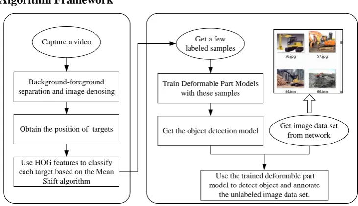
Figure 1. Schematic algorithm framework.
As shown in Figure.1, with the targets as foregrounds, this paper gets the position of the targets based on the Gaussian mixture model, then the HOG features of the targets is clustered based on the Mean Shift clustering algorithm to obtain the categories, and subsequently the labeled samples obtained in the above steps is used to train the deformable part model so as to get the detection model. Finally a large number of unlabeled images can be annotated with the trained deformable part model. In essence, this paper uses weaker classifiers to annotate samples and reinforces labeling information layer by layer, so as to find more significant structural features from a small number of samples and label more samples.
Prepared Work Video Capture
This article focuses on an automatic annotation algorithm for deep learning image datasets based on HOG features. The video is captured firstly (the video shown in Figure.2 can be downloaded from http://wordpress-jodoin.dmi.usherb.ca/dataset2014/). With the pedestrian as the target to be classified, this article selects a pedestrian mo-tion scene taken by a fixed surveillance camera and obtains a pedestrian dataset as shown in Figure.2.
Figure 2. A sample video and the frames.
Foreground Extraction and Denoising Processing
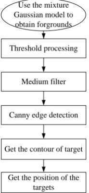
[image:2.595.199.411.564.686.2]shown in Figure.3. Furthermore, there are many cases where dynamic backgrounds are included in nature such as leaf shaking or water ripples. As shown in the video in Figure.2, the water surface in the back-ground is dynamic, and the pedestrian foreground extracted by the Gaussian mixture model still contains these noises, so the threshold processing and the median filter are used to process the foreground noise.
Use the mixture Gaussian model to
obtain forgrounds
Threshold processing
Medium filter
Canny edge detection
Get the contour of target
[image:3.595.252.345.144.344.2]Get the position of the targets
Figure 3. Foregrounds location acquisition process.
[image:3.595.186.412.367.437.2]
(a) (b) (c)
Figure 4. (a) The foreground extracted by Gaussian mixture model (b) The foreground after denoising (c) The bounding box of the foreground.
The foreground extracted by the Gaussian mixture model is shown in Figure. 4(a). The foreground after the threshold processing and the median filter is shown in Figure. 4(b). After denoising processing, the noise of the dynamic background is suppressed, a clean foreground can be obtained. As shown in Figure. 4(c), the canny algorithm is used to calculate the contour to get the minimum bounding box. The position information mainly contains four parameters: xmin, ymin, xmax, ymax. The four parameters respectively represent the x, y coordinates of the pixel points in the upper left corner and in the lower right corner of the bounding box. Then the same processing on all video frames is performed to obtain their location. The specific data is shown in Table 1.
Table 1. The position of the target.
Picture name xmin ymin xmax ymax
image17.jpg 31 13 51 113
image18.jpg 31 13 59 113
image19.jpg 33 15 60 115
image20.jpg 35 15 59 114
image21.jpg 38 14 56 106
Mean Shift Clustering Algorithm Based on HOG Feature
HOG Feature
calculating and counting histograms of gradient directions in the local area of the image. The basis is that the shape of the detected local object can be described by the gradient of the intensity of the light and the distribution of the edge direction. The essence is the statistical information of the gradient, and the gradient always exists at the edge of the image (the edge is composed of the points where the brightness changes obviously in the image.).
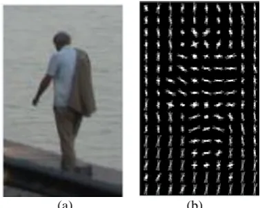
As shown in Figure. 5, Figure. 5(a) is a raw image (the picture is selected from the PASCAL VOC dataset), and Figure. 5(b) is a visual image of the HOG feature, and the gradient information of the pedestrian can be seen clearly.
(a) (b)
Figure 5. (a)The raw image (b) HOG feature visualization.
Mean Shift Clustering Algorithm
Mean Shift algorithm [10] is a non-parameter estimation algorithm or nuclear density estimation algorithm. It is an effective iterative algorithm, which makes each point in the local point move? to the direction with the highest probability density. This paper uses the Mean Shift algorithm to cluster HOG features to distinguish different kinds of objects. Consider a d-dimensional space as a sphere, then given a set of n data points in the d-dimensional space, and the basic form of the Mean Shift vector for any point x in space is expressed as Eq.1:
1
( )
i k
h i
x S
M x x
K
(1) This vector is the Mean Shift vector, where Sk represents the data point in the dataset whose
distance to x is less than the length h of the bandwidth, expressed as Eq.2:
2
( ) : ( ) (T )
h i i
S x y y x y x h
(2) Update the position of the center x by calculating the Mean Shift vector, the updated center x is expressed as Eq.3:
h
x x M
[image:4.595.203.392.199.350.2]2 1 2 1 m(x)= n i i i n i i x x x g h x x x g h
(4)Therefore, the updated spherical center coordinate is expressed as Eq.5:
2 1 2 1 ( ) ( ) n i i i n i i x x x g h x x x g h
(5) The main idea of Mean Shift is to divide the value field of data into several equal intervals. The data is divided into several groups by interval, forming a histogram of the probability distribution of the corresponding data. The algorithm is robust to initialization and has a large overhead in computation time. It is more effective for data with lower dimensions. As the dimension increases, the corresponding calculation amount of the histogram will also increase, directly affecting the real-time performance of the algorithm. Therefore, in this paper, the target to be labeled is uniformly compressed to 256*256 pixels after the position of the target is obtained by the background separation algorithm, so the dimension of the HOG features is reduced. Then the Mean Shift clustering algorithm based on the HOG feature can improve the speed of calculations. The Mean Shift algorithm in this paper has only one parameter, bandwidth parameter h, so the choice of h has a great influence on Mean Shift algorithm. In this paper, bandwidth is calculated by the bandwidth estimation method. In essence, it is the average farthest k nearest neighbor distance.Deformable Part Models
After the above steps, a few labeled image data can be obtained, which is not enough for deep learning training. In general, the quality of the sample dataset is directly related to the training effect of the deep learning model. If the sample size is not enough, the model will be overfitted, resulting in weak generalization ability. Therefore, this article firstly uses the above method to obtain a small amount of labeled image data, then uses these data as training data to train the deformable part model. After the classification model is obtained, the unlabeled pictures can be annotated so that we can get more labeled data.
The Deformable Part Model (DPM) (Felzenszwalb et al., 2008) was proposed by Felzenszwalb in 2008 [11]. It is a part-based detection method so that it is robust to the deformation of the target. At present, DPM has become a core part of many algorithms for classification, segmentation, pose estimation, etc. Because of the relatively lesssamples required, this paper applies it to the object detection of images to obtain more labeled datasets.
Experimental Design and Analysis
Experiment One: Using Mean Shift Clustering Algorithm to Classify Targets of Different Categories
A video containing categories of people and digger is used to create labeled datasets. The main design flow of the experiment is as follows:
(1) Using the Gaussian mixture model for foreground extraction; (2) Denoising processing;
(4) Calculating the HOG features of the target after getting its position; (5) Using Mean Shift algorithm to cluster targets based on HOG features.
20 frames of the video is taken for the clustering experiment, and an example frame in the video is shown in Figure 6(a). The Table 2 shows that the change of the 20 frames’ clustering results as bandwidth increases. Repeated experiments show that when the proportion of the neighbor samples is set to 0.2~0.525 in the neighborhood search which means the bandwidth is between 5.69 and 8.52, the algorithm can effectively cluster digger and pedestrian to distinguish them accurately.
Table 2. The effects of bandwidth on clustering results.
bandwidth 5.59 5.69 8.52 8.53
proportion of properly clustered objects
23/40 40/40 40/40 20/20
It can be clearly seen from the data in Table 2 that using Mean Shift clustering can quickly classify different categories according to HOG features, reducing the amount of calculationand speeding up the classification speed. This method do not need to rely on human to create labels and as a consequence, it can reduce human’s burden.
The clustering resulte of a frame is shown in Figure 6(b).
(a) (b)
Figure 6. (a) The raw frame (b) The clustering results of different categories.
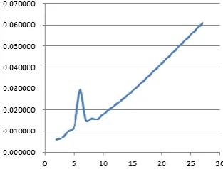
[image:6.595.124.476.313.421.2]Time-consuming curve of Meanshift algorithm as the total amount of hog features increases is shown in the Figure 7. The horizontal axis represents the number of video frames, and the vertical axis represents the time it takes for the meanshift to cluster the targets in the video frame.
Figure 7. Time-consuming curve of Meanshift algorithm as the total amount of hog features increases.
Experiment Two: Training a Deformable Part Model with a Few Samples to Obtain More Labeled Data
Experience shows that compared with pedestrian detection, digger detection is a more difficult task, so this experiment takes digger samples as an example to show the results of using DPM to obtain more labeled data. The main design flow for the experiment is as follows:
(1) Rely on experiment one to obtain a small number of labeled samples, these samples are used as training data. In this paper, the number of positive samples is 1000, and the number of negative samples is also 1000;
[image:6.595.218.375.494.613.2](3) Obtain unlabeled pictures of the digger from the network and use them as a test set;
[image:7.595.141.458.139.302.2](4) Use the digger detection model to detect digger in the test set. The detection results is shown in Figure.9, from which the annotation xmin, ymin, xmax, ymax can be obtained. In this way, more digger labeled data can be obtained.
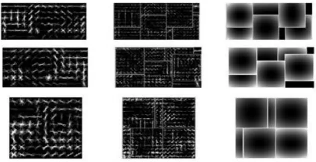
[image:7.595.157.440.329.483.2]Figure 8. The visualization of digger detection model (a) The root filter (b) The part filters (c) The anchor of part filters.
Figure 9. The detection performance of digger DPM model on the test date set.
Table 3. The precision and recall of digger detection models with different thresholds.
Threshold Precision Recall
0.5 84.2% 68.8%
0.6 89.2% 80%
0.7 93.6% 92.49%
It can be clearly seen from the data in Table 3 that setting different thresholds has a great effect on the detection of diggers. After a series of reliable experiments, the results show that when the threshold is set to 0.7, the precision and recall reach a good value, so the 93.6% of the samples which are correctly classified can be used as positive samples of the digger, and at the same time the position of digger in each image can be obtained.
Conclusion
object detection model. Thereby, we can detect more unlabeled pictures and obtain more labeled samples with the trained DPM. In essence, this paper uses weaker classifiers to annotate samples and reinforces labeling information layer by layer, so as to find more significant structural features from a small number of samples, and uses these features to label more samples. In the cases of that a small amount of misjudgment, rapid screening can be performed by human. In summary, this paper realizes the automatic annotation of image datasets in deep learning, improving the work efficiency of annotation, and reducing the cost of acquiring image data sets.
References
[1] LeCun Y, Bengio Y, Hinton G. Deep learning[J]. nature, 2015, 521(7553): 436. [2] LabelImg GitHub [2017]. URL: https://github.com/tzutalin/labelImg.
[3] puzzledqs. Bbox-label-tool. https:https://github.com/puzzledqs/BBox-Label-Tool, 2014.
[4] Klein B, Lev G, Sadeh G, et al. Associating neural word embeddings with deep image representations using fisher vectors[C]//Proceedings of the IEEE Conference on Computer Vision and Pattern Recognition. 2015: 4437-4446.
[5] Goodfellow I, Pouget-Abadie J, Mirza M, et al. Generative adversarial nets[C]//Advances in neural information processing systems. 2014: 2672-2680.
[6]Xiao L, He K, Zhou J, et al. Image noise removal on improvement adaptive medium filter [J][J]. Laser Journal, 2009, 2: 018.
[7] Green B. Canny edge detection tutorial[J]. Retrieved: March, 2002, 6: 2005.
[8] Reynolds D. Gaussian mixture models[J]. Encyclopedia of biometrics, 2015: 827-832.
[9] Dalal, Navneet, and Bill Triggs. "Histograms of oriented gradients for human detection." Computer Vision and Pattern Recognition, 2005. CVPR 2005. IEEE Computer Society Conference on. Vol. 1. IEEE, 2005.
[10]Comaniciu D, Meer P. Mean shift: A robust approach toward feature space analysis[J]. IEEE Transactions on pattern analysis and machine intelligence, 2002, 24(5): 603-619.