Volume 2008, Article ID 396126,11pages doi:10.1155/2008/396126
Research Article
Ring-Based Optimal-Level Distributed Wavelet Transform with
Arbitrary Filter Length for Wireless Sensor Networks
Siwang Zhou,1Yaping Lin,1and Yonghe Liu2
1School of Software, Hunan University, Changsha 410082, China
2Department of Computer Science and Engineering, The University of Texas at Arlington, Arlington, TX 76019, USA
Correspondence should be addressed to Yaping Lin,[email protected]
Received 1 May 2007; Revised 31 August 2007; Accepted 8 November 2007
Recommended by Huaiyu Dai
We propose an optimal-level distributed transform for wavelet-based spatiotemporal data compression in wireless sensor net-works. Although distributed wavelet processing can efficiently decrease the amount of sensory data, it introduces additional com-munication overhead as the sensory data needs to be exchanged in order to calculate the wavelet coefficients. This tradeoffis ex-plored in this paper with the optimal transforming level of wavelet transform. By employing a ring topology, our scheme is capable of supporting a broad scope of wavelets rather than specific ones, and the “border effect” generally encountered by wavelet-based schemes is also eliminated naturally. Furthermore, the scheme can simultaneously explore the spatial and temporal correlations among the sensory data. For data compression in wireless sensor networks, in addition to minimizing energy and consumption, it is also important to consider the delay and the quality of reconstructed sensory data, which is measured by the ratio of signal to noise (PSNR). We capture this withenergy×delay/PSNRmetric and using it to evaluate the performance of the proposed scheme. Theoretically and experimentally, we conclude that the proposed algorithm can effectively explore the spatial and temporal corre-lation in the sensory data and provide significant reduction in energy and delay cost while still preserving high PSNR compared to other schemes.
Copyright © 2008 Siwang Zhou et al. This is an open access article distributed under the Creative Commons Attribution License, which permits unrestricted use, distribution, and reproduction in any medium, provided the original work is properly cited.
1. INTRODUCTION
Edging toward real world deployments, wireless sensor net-works have revealed vast potentials in a plethora of appli-cations including battle field monitoring, environmental ex-ploration, and precision agriculture [1,2]. Owing to the se-vere resource constraints such as memory space, computa-tion power, and communicacomputa-tion bandwidth, gathering all the raw, original sensory data is not often feasible in wireless sen-sor networks. Motivated thereby, extensive research efforts have been focusing on wavelet data compression in wireless sensor networks, with a goal of data amount reduction and hence energy conservation. For example, the WISDEN sys-tem [3] is designed for structural monitoring. In this sys-tem, wavelet compression is first performed in a single sen-sor node and the wavelet coefficients are then sent for fur-ther processing at a central location. Aiming at time-series sampled by a single sensor node, RACE [4] proposes a rate adaptive Haar wavelet compression algorithm. The support of Haar wavelet is 1 and its structure is simple. As a result,
the algorithm can be executed efficiently. However, the above wavelet-based approaches do not exploit the fact that data originated from physically proximate sensors are often highly correlated. Consequently, energy can be wasted due to the transmission of redundant data. Dimensions [5,6] propose a hierarchical routing scheme with its wavRoute protocol. This scheme exploits the temporal data redundancy at the bottom level of the routing hierarchy firstly, and then performs spa-tial data reduction in the middle. Still, there exists the trans-mission of spatially redundant data from the bottom to the middle of the hierarchy.
the “border effect” particularly. Transforming level is another important property of wavelet transform. Although higher compression efficiency can be obtained along with increas-ing transformincreas-ing levels, additional energy and delay cost are introduced as more sensory data need to be exchanged to perform the transform. Therefore, it is important to look for the optimal transforming levels in conjunction with proper topology. Although Haar wavelet-based adaptive level mul-tiresolution representation is proposed in [10], the scheme is difficult to generalize to wavelet function with arbitrary length support. Moreover, the scheme has ignored network delay, which is crucial for certain applications. Performance evaluation of distributed WT algorithms is also an interesting problem. In [9], irregular WT is studied and its performance is evaluated using “mean square error” (MSE) and energy metrics separately. On the contrary, in [7–10], the metrics of evaluation involve many aspects, such as energy consump-tion, reconstruction quality metric, delay, and so on. How-ever, they only use those metrics unilaterally without con-sidering their relation. This, in turn, has also limited their performance and application scope.
Motivated thereby, in this paper, we propose a ring topology-based, optimal-level distributed transform for wavelet functions, whose support length can be arbitrary. Our scheme simultaneously exploits the spatial and tempo-ral correlation residing in the sensor data within clusters. The ring model will naturally eliminate the “border effects” encountered by WT and hence further strengthen its sup-port to general wavelets. Furthermore, our scheme is capa-ble of accommodating a broad range of wavelets which can be designated by different applications. Moreover, we pro-pose a scheme of optimal level of WT, which can explore the tradeoffbetween the benefit of distributed WT and the cor-responding overhead. We evaluate the performance of data compression for sensor networks withenergy×delay/PSNR
metric, which gives enough consideration in the tradeoffof energy consumption, network delay, and the quality of re-constructed sensory data. Theoretically and experimentally, we analyze the performance of our proposed algorithm and perform comparison with other schemes.
The remainder of this paper is organized as follows. In
Section 2, we first study the border effect in sensor networks, then detail the ring model and describe the optimal WT thereon. InSection 3, we present the performance evaluation model for data compression in sensor networks, and then an-alyze the performance of the proposed framework. Experi-mental study is presented in Section 4and we conclude in
Section 5.
2. SPATIAL-TEMPORAL WAVELET COMPRESSION
In this section, we first examine the potential impact of bor-der effect on sensory data reconstruction in sensor networks, and then present the network model and the construction of the virtual ring topology to eliminate the border effect. Sub-sequently, the optimal transforming-level-based algorithm for compressing spatial and temporal correlated data is de-tailed.
2.1. Border effect in sensor networks
We assume that sensory data collected are stored in each sen-sor node in a distributed fashion. While these data can be compressed employing wavelet based on one-dimensional network model [2], border effect will induce errors when re-constructing the sensing field. If the reconstructed data are different from the original data, the results are considered to be distortive.
For general wavelet functions with arbitrary supports, let their lowpass and corresponding highpass analysis filter be
Ln,−i1≤n≤ j1, i1≥0, j1>0,
Hn,−i2≤n≤ j2, i2≥0, j2>0.
(1)
Let
L=maxi1+j1+ 1,i2+j2+ 1, (2)
I=maxi1,i2, (3)
J=maxj1,j2. (4)
As a consequence of border effect, we have the following the-orem.
Theorem 1. Performing K-level distributed WT on sensory data stored inNsensor nodes, if2K((2K−
1)I/2K+(2K−
1)(J−1)/2K) + (2K−
1)(I+J−1)< N, whereis a opera-tor of bounding, then the sensor nodes whose reconstructed data are distortive amount to2K((2K −1)I/2K+(2K−1)(J−
1)/2K) + (2K−1)(I+J−1), otherwise, the reconstructed sen-sory data in allNsensor nodes will be distortive.
Proof. The sensory data stored inNsensor nodes can be re-garded as a one-dimensional array withNelements. Using wavelet function as defined by (1)–(4), we performK-level WT on the one-dimensional array. According to the decom-position steps of Mallat algorithm [11]
xi+1
k =
n
Ln−2kx(ni),
di+1
k =
n
Hn−2kxn(i),
(5)
wherei≥0,xi+1
k anddik+1is thekth approximation and detail
coefficients in the (i+1)th level WT, respectively. If the border of the array is not extended, the distortive detail coefficients in theKth level WT will amount to
2K−1i1 2K
+ 2
K
−1j1−1 2K
. (6)
The distortive approximation coefficients correspondingly are
2K−1i2 2K
+ 2
K
−1j2−1 2K
. (7)
According to the reconstruction steps of Mallat algorithm,
xi
n=
k
Ln−2kxki+1+
k
M
N
Figure1: Ring topology based on virtual grid.
Along with (3) and (4), the total number of the distortive sensory data becomes
Num=2K 2
K −1I 2K
+ 2
K
−1(J−1) 2K
+2K−1(I+J−1).
(9)
This shows that the sensory data reconstructed are dis-tortive as compared to those originally stored in the sensor nodes. For simplicity, we consider wavelet function to have the same analysis and synthetic filters. Obviously, if Num ≥N, allNreconstructed sensory data are distortive.
Here, we give a simple example to illustrate the border effect. Assume that the number of nodes in a network is 400, and a 3-level WT on the sensory data employing Daubechies 9/7 wavelet is performed. There will be 105 nodes whose re-constructed data are distortive according toTheorem 1. This accounts to around a quarter of all the sensor nodes. From
Theorem 1and this example, we conclude that the border effect can potentially have significant impact on the recon-struction of sensory data.
2.2. Ring topology based on virtual grid
Below, we describe a ring topology based on virtual grid. As we will illustrate later, ring-topology-based WT can elimi-nate border effect and can fully explore the spatial correlation among sensory data.
2.2.1. Virtual grid and data correlation model
We assume that the sensor network is divided into different clusters, each of which is controlled by a cluster head [12]. Our focus is given to energy-efficient gathering of the sen-sory data from various cluster members to the cluster head. Routing the data from the cluster head to the sink is out of the scope of this paper although it may benefit from the com-pression algorithm presented in this paper. We assume that in a cluster, nodes are distributed in a virtual grid as illustrated inFigure 1. The distance among nodes can be estimated ac-cording to the distance among the corresponding grid cells. It can also be calculated according to the factual positions of the nodes. The division of cells in a cluster relies on the net-work topology and node density. We assume that one cell at
least contains one node and in each cell, one node is selected as the reporting node (for reporting the data to the cluster head).
Without confusion, we will simply use node to refer to this reporting sensor. We remark that this model is neither restrictive nor unrealistic. In the worst case, a single node can logically reside in one grid cell and can be required to report its data corresponding to every query or during every specified interval.
There exists a certain correlation for the sensory data stored in each node, which can be described using a corre-lation model. Let correcorre-lation coefficientρrepresent the data correlation and letrsrepresent correlation scope. In
correla-tion model,ρwill be zero if the distance between two nodes exceedsrs. If the distance isd(d < rs), thenρ=1−d/rs.
2.2.2. Ring topology based on virtual grid
The key for our construction is that we form a ring topology among the reporting sensor nodes, as illustrated inFigure 1. To do this, we initially select a node randomly as the ring head, and then determine a neighboring node as its next node. This neighbor-selection procedure will be repeated un-til the ring topology is completed. In order to maximize the correlation among neighboring nodes and hence the effect of compression, the ring can be computed in a centralized man-ner by the cluster head and broadcast to all nodes. Notice that multiple rings may be available due to node density.
In this ring topology, neighboring nodes belong to spa-tial adjacent grid cells. A node on the ring receives data from one of its neighbors, fuses the data with its own, and fur-ther forward the results to the ofur-ther neighbor. As the nodes are relaying the sensory data, WT will be executed and cer-tain wavelet coefficients will be actually stored locally and some others will be forwarded. Indeed, nodes in a particu-lar grid cell can alternatively participate in the ring and hence the data-gathering procedure. This way, energy consumption can be more evenly distributed among the nodes and thus extend the network lifetime. Readers are referred to [13] for approaches of scheduling nodes within one grid, for exam-ple, power on and off, for this purpose.
Given the ring topology, in each data gathering round, a node will be chosen as the “head” of the ring and the nodes will be indexed accordingly ass0,s1,. . .,si,. . .,sN−1, whereN is the number of nodes on the ring. In addition, we assume that sensoristores datacji,j=0, 1,. . .,M−1, wherejis the
temporal index andcjirepresents the sensory data of sensor
i at time index j. Evidently, dependent onM, each sensor will window out history data. Accordingly, we can arrange the sensory data on the ring according to their spatial and temporal relationship to a matrixC0= {cji}, 0≤i < N, 0≤ j < M, where columnirepresents the data of sensor nodei. For ease of notation, we will useCito denote columni.
We remark that while extensive data-gathering struc-tures have been studied in the literature, they are usually tree-based. Undeniably, the ring construction requires care-ful study in order to best benefit from its special properties. While considering this as our future work, we provide here a brief discussion. First of all, due to the procedure of dis-tributed wavelet compression, it is desirable to have higher data correlation among neighboring nodes. This way data can be better compressed while being forwarded along the ring and hence energy can be saved. Often, this can be nat-urally satisfied by selecting physically proximate nodes to be neighbors on the ring. At the same time, the longer the ring, the more compression can possibly be achieved. However, with increasing the length of the ring, the number of wavelet coefficients will also increase which can in turn introduce ad-ditional calculation and storage cost. Adad-ditionally, network delay for data gathering will also increase as the ring length increases. Balancing the size of the ring and the number of the rings will require careful tradeoffamong all the above-mentioned factors.
2.3. VGRT-based optimal level spatial-temporal wavelet transform
2.3.1. Spatial-temporal wavelet transform
Our goal is to employ the WT for compressing sensory data on the ring so that it can be energy efficiently transmitted to the cluster head. The approach is to simultaneously ex-ploit the temporal and spatial correlation among the nodes’ data and reduce the redundancy thereby. As the data is repre-sented by matrixC0, the temporal (within a node) and spa-tial (among multiple nodes) correlations are then captured by the columns and rows, respectively. Correspondingly, in our design, we will first perform WT on each column and then perform WT on the rows. Furthermore, these column WT and row WT can be performed recursively to achieve a K-level WT. Notice that column WT is within a single node hence no communication is required although data will be buffered. On the contrary, the row WT is among the sensor nodes and hence requires additional communications.
Our first step is to perform transform on the columns of C0to exploit temporal correlation. LetL
nandHnbe lowpass
and highpass analysis filters, respectively, we have
c1,mL,i=
n
L(n−2m)Ci(n),
cm1,H,i =
n
L(n−2m)Ci(n), 0≤m≤N/2,
(10)
where C1,mL,i represents the mth approximation wavelet
co-efficient in theith column in the first level of the column WT,Cm1,H,i is the corresponding detail wavelet coefficient, and
Ci(n) denotes thenth element ofCi. Notice that this
trans-form is pertrans-formed within each node on its own sensory data and thus does not require any communication among the
nodes on the ring. Subsequently, we can realign the resultant wavelet coefficients and obtain matrix
C1= ⎧ ⎪ ⎪ ⎪ ⎪ ⎪ ⎪ ⎪ ⎪ ⎪ ⎪ ⎪ ⎪ ⎪ ⎨ ⎪ ⎪ ⎪ ⎪ ⎪ ⎪ ⎪ ⎪ ⎪ ⎪ ⎪ ⎪ ⎪ ⎩
c1,0,0L c1,
L
0,1 · · · c1,
L
0,N−1 ..
. ... . .. ... c1,M/L2−1,0 c
1,L
M/2−1,1 · · · c 1,L M/2−1,N−1
c1,0,0H c1,0,1H · · · c1,0,NH−1 ..
. ... . .. ... c1,M/H2−1,0 c1,M/H2−1,1 · · · c1,M/H2−1,N−1
⎫ ⎪ ⎪ ⎪ ⎪ ⎪ ⎪ ⎪ ⎪ ⎪ ⎪ ⎪ ⎪ ⎪ ⎬ ⎪ ⎪ ⎪ ⎪ ⎪ ⎪ ⎪ ⎪ ⎪ ⎪ ⎪ ⎪ ⎪ ⎭ . (11)
Given matricC1, our second step is to perform WT on its rows to explore the spatial correlation among the nodes. Note that the first and the last columns are adjacent on the ring topology, and this resembles a periodic extension to the sig-nal. Towards this end, for general wavelets with arbitrary supports whose lowpass analysis filter isLn,−i1 ≤ n < j1
and highpass analysis filter is Hn, −i2 ≤ n < j2, where
i1,i2,j1,j2 ≥ 0, we analyze the different cases of the row transform based on whetherj1andj2are even or odd.
Case 1. If j1is even and j2is odd, by performing WT on the rows in a similar way to the column WT, we obtain
C2= ⎧ ⎪ ⎪ ⎪ ⎪ ⎪ ⎪ ⎪ ⎪ ⎪ ⎪ ⎪ ⎪ ⎪ ⎪ ⎨ ⎪ ⎪ ⎪ ⎪ ⎪ ⎪ ⎪ ⎪ ⎪ ⎪ ⎪ ⎪ ⎪ ⎪ ⎩
c1,0,LLl0 c
1,LH
0,h0 · · · c
1,LL
0,lN/2−1 c
1,LH
0,hN/2−1
..
. ... . .. ... ... c1,M/LL2−1,l0 c
1,LH
M/2−1,h0 · · · c
1,LL
M/2−1,lN/2−1 c
1,LH M/2−1,hN/2−1
c1,0,HLl0 c
1,HH
0,h0 · · · c
1,HL
0,lN/2−1 c
1,HH
0,hN/2−1
..
. ... . .. ... ... c1,M/HL2−1,l0 c
1,HH
M/2−1,h0 · · · c
1,HL
M/2−1,lN/2−1 c
1,HH M/2−1,hN/2−1
⎫ ⎪ ⎪ ⎪ ⎪ ⎪ ⎪ ⎪ ⎪ ⎪ ⎪ ⎪ ⎪ ⎪ ⎪ ⎬ ⎪ ⎪ ⎪ ⎪ ⎪ ⎪ ⎪ ⎪ ⎪ ⎪ ⎪ ⎪ ⎪ ⎪ ⎭ , (12)
where li = ((N− j1 + 2i)/2 modN/2), hi = ((N− j2+
2i+ 1)/2 modN/2),c1,LL
m,n andc1,mHL,n represent the
approxi-mation coefficients in the first level of the row WT, andc1,LH m,n
andc1,HH
m,n represent the corresponding detail coefficients. We
remark that for a node with index i, if iis even, the node stores coefficientsc1,mLL, (N−j1+i)/2 modN/2andc1,mHL, (N−j1+i)/2 modN/2; ifiis odd, the node stores coefficientsc1,mLH, (N−j2+i)/2 modN/2and c1,mHH, (N−j2+i)/2 modN/2, 0≤m≤M/2−1. Notice that this
trans-form is pertrans-formed among the sensor nodes on the ring to harvest the spatial correlation and hence resultant wavelet coefficients cannot be realigned as in the column WT.
Based on the approximation coefficients inC2, we can obtain matrixC1as
C1= ⎧ ⎪ ⎪ ⎪ ⎪ ⎪ ⎪ ⎪ ⎨ ⎪ ⎪ ⎪ ⎪ ⎪ ⎪ ⎪ ⎩
c1,0,LLl0 c
1,LL
0,l1 · · · c
1,LL
0,lN/2−1
c1,1,LLl0 c
1,LL
1,l1 · · · c
1,LL
1,lN/2−1
..
. ... . .. ... c1,M/LL2−1,l0 c
1,LL
M/2−1,l1 · · · c
1,LL M/2−1,lN/2−1
We can perform the second-level column and row WT on matrixC1as those to matrixC0and extend to theKth level spatiotemporal WT similarly.
Once the K-level WT is performed, the original data gathered by the nodes on the ring is transformed to the wavelet domain. Since the spatial and temporal correlations are exploited, we can represent the original data using fewer bits. In lossless compression, all the wavelet coefficients will be encoded and sent to the cluster head; in lossy com-pression, according to different application-specific require-ments, the wavelet coefficients can selectively be encoded and sent to the cluster head by different nodes.
Case 2. If j1andj2are both odd, while we can perform the transform following similar procedure, the matrices will be significantly different. Due to space limitation, we omit them here but remark that those nodes whose indexes are odd will not store wavelet coefficients.
When we perform row WT, the first group of approx-imation coefficients is calculated using the data stored in the ((N−i1) modN)th node to the (j1modN)th node and are stored in the (j1modN)th node. The corresponding de-tail coefficients are calculated using the data stored in the (N−i2)th node to the (j2modN)th node and are stored in the (j2modN)th node. Whenj1is odd andj2is even, it will be similar to the first case, and whenj1andj2are both even, it will be similar to the second case discussed above.i1andi2 will not affect the distribution of wavelet coefficients.
2.3.2. Optimal transforming level of wavelet function
In this subsection, we will study how many transforming levels needed to be performed to obtain optimal network performance. We evaluate network performance with energy and delay.
From data compression’s point of view, WT is desired only if the average number of encoding bits of wavelet co-efficients can be reduced. LetBk−1andBkbe the average
en-coding bits of wavelet coefficients in the (k−1)th and thekth level, respectively, then we have
Bk−1−Bk= f(data, wavelet). (14)
Since most of energy consumption is data transmission and most of delay factor is in the transmission time for wire-less sensor networks, we measure energy and delay in terms of the size of data being transmitted. We might as well denote e(·) andd(·) are energy and delay cost function respectively. Studying the optimal transforming level of spatial-temporal WT, we have the following theorem.
Theorem 2. LetEk,INandDk,INbe the additional energy and delay cost by distributed spatial-temporal thekth-level WT, re-spectively,K1 = max (k : Ek,IN−e(Bk−1−Bk) ≤ 0),K2 =
max (k:Dk,IN−d(Bk−1−Bk)≤0), then the optimal trans-forming level of spatial-temporal WTKisK=min (K1,K2).
Proof. The energy consumption and delay of sending (Bk−1− Bk) bits data ise(Bk−1−Bk) andd(Bk−1−Bk), respectively.
If the energy and delay cost generated by thekth level WT
are all less than or equal to that of the (k−1)th level WT, then thekth level WT would be performed. So we can easily obtainTheorem 2.
The optimal transforming level of wavelet function can be calculated distributively by the nodes on the ring. With-out loss of generality, we assume that the energy function e(·) and delay functiond(·) have been loaded to nodes in advance. The energy and delay are calculated by nodes dur-ing they perform WT. Each node forwards the value of energy and delay while the data are sent to the next node to produce wavelet coefficients. So the node, which stores the last col-umn wavelet coefficients, knows the total energy and delay cost in the corresponding transforming level, and thus it can decide if the next transforming level will be performed. If the decision is “YES,” then the new level WT will be initiated by the node that stores the first column wavelet coefficients. The decision can be easily transmitted to the node thanks to the ring topology.
2.4. Discussion
In the above WT, the ring head can be alternated among dif-ferent nodes when performing the data-gathering procedure. Consequently, the wavelet coefficients will be distributed to different nodes accordingly which in turn will balance the energy consumption within the cluster. Furthermore, neigh-boring nodes on the ring belong to spatial adjacent virtual grids, so the data gathered by the neighboring nodes are more likely spatially correlated. Because the calculation of approximation and detail wavelet coefficients are for neigh-boring nodes within a support length, performing WT based on the ring can make full use of spatial correlation to remove the data redundancy and hence reduce transmission cost.
More importantly, performing WT based on ring topol-ogy naturally eliminates the “border effect” problem inher-ent in WT. It is well known that general wavelet functions are defined on the real axisRwhile the signal is always limited in a finite regionK. Therefore, the approximate spaceL2(R) will not match the signal spaceL2(K) which will result in the “border effect” and thus introduce errors during signal re-construction. One of the general methods to deal with “bor-der effect” is extending border. The ring topology resembles a periodic extension to the signal that naturally dissolves the “border effect.”
Before going forward, we remark here that our scheme aims at traditional wavelet transform and hence is not di-rectly applicable to the second-generation wavelet. Moreover, due to the strick requirement of the topology for data for-warding, the scheme lacks robustness in its current form. These are considered our future work.
3. PERFORMANCE EVALUATION
3.1. Energy consumption and delay analysis
We now briefly analyze the total energy consumption and de-lay of the proposed scheme. For this purpose, we adopt the first-order radio model described in [12]. In this model, a ra-dio dissipatesEelecamount of energy at the transmitter or re-ceiver circuitry andampamount of energy for transmit am-plifier. Signal attenuation is modeled to proportional tod2 on the channel, whereddenotes distance. Forkbits data and a distanced, the transmission energy consumptionETx and reception energy consumptionERxcan be calculated, respec-tively, as
ETx(k,d)=ETx-elec(k) +ETx-amp(k,d),
ETx(k,d)=Eelec×k+amp×k×d2,
ERx(k)=ERx-elec(k)=Eelec×k.
(15)
We further assume that the sensor nodes can transmit simultaneously and neglect the processing and propagation delay. Let the transmission time of one data unit be one unit time. Let EIN and DIN represent the energy consumption and delay resulting from communication among the nodes within the cluster for performing the proposed WT. We can derive the following theorem.
Theorem 3. For general wavelets with arbitrary supports, let the lowpass analysis filter beLn,−i1≤n < j1, and let the high-pass analysis filter beHn,−i2≤n < j2, wherei1,i2,j1,j2 ≥0. For aK-level distributed spatiotemporal WT based on the ring topology proposed above, to gather the sensory data in a cluster ofNnode,
EIN=EWAV+EOPT, (16)
DIN=
K
n=1
max 0≤l≤N/2n−1
i1+j1−1
i=0
qLinl+BL
+ max 0≤l≤N/2n−1
i2+j2−1
i=0
qHinl+BH
+N−2nBL+BH
,
(17)
where
EWAV
= K
n=1
N/2n−1
l=0
EPn,l+2Eelec
i1+j1+1
i=0
qLinl+BL
+
i2+j2+1
i=0
qinlH+BH
+amp i1+j1+1
i=0
qL
inl+BL
·dL
inl
+
i2+j2+1
i=0
qH
inl+BH
·dH
inl
,
EOPT= K
n=1
2EelecBLN−2n+BHN−2n
+amp
−i1+N+2(n−1)l+(2n−1−1)(i1+j1)+N−2n−1
j=−i1+N+2n−1l+(2n−1−1)(i1+j1)
BL·d jmodN
+
−i2+N+2(n−1)l+(2n−1−1)(i2+j2)+N−2n−1
j=−i2+N+2n−1l+(2n−1−1)(i2+j2),
BH·d jmodN
qL
inl=qLn,(−i1+N+2nl+(2n−1−1)(i1+j1)+2n−1i) modN,
qinlH =qHn,(−i2+N+2nl+(2n−1−1)(i2+j2)+2n−1i) modN,
qL
inl=
−i1+N+2nl+(2n−1−1)(i1+j1)+2n−1−1
j=−i1+N+2nl+(2n−1−1)(i1+j1)
dj mod N
2 ,
qH
inl=
−i2+N+2nl+(2n−1−1)(i2+j2)+2n−1−1
j=−i2+N+2nl+(2n−1−1)(i2+j2)
dj mod N
2 .
(18)
EWAVandEOPTare the energy consumption for producing the wavelet coefficients and forwarding the values of energy and delay, respectively. BLandBH are the bit number storing the value of energy and delay, introduced by the production of low- and high-wavelet coefficients, respectively. qLn,i and qHn,i are the data amount transmitted by the ithnode when the lthapproximation coefficient and the corresponding detail co-efficient in thenthlevel row WT are calculated, respectively, djmodN is the distance between the(jmodN)thnode and the
((j+ 1) modN)thnode,EPn,lis the processing energy of when thelthwavelet coefficients are calculated in thenthlevel WT.
Proof. When thelth approximation wavelet coefficient in the nth level row WT is calculated, the transmitting costELn,lis
ELn,l=ETx+ERx=2Eelec i1+j1
i=0 qLinl
+amp
i1+j1
i=0
qLinl·dLinl
.
(19)
When thelth detail wavelet coefficient in thenth level row WT is calculated, the transmitting costEH
n,lis
EH
n,l=2Eelec i2+j2
i=0 qH
inl+amp
i2+j2
i=0
qH
inl·dHinl
. (20)
When thenth level WT is performed, the processing costEp
is
EP= N/2n−1
l=0
EnP,l. (21)
Then, ifK-level WT are performed, the energy costEINis
EIN= K
n=1
Ep+ N/2n−1
l=0
EL n,l+EHn,l
Taking (19), (20), and (21) into (22), we can obtain (16). In the system of CDMA, the communication interference among nodes is little, so the wavelet coefficients can be cal-culated simultaneously. The network delay of thenth WT is
DIN= max
0≤l≤N/2n−1
i1+j1−1 l=0 q
L
inl
+ max 0≤l≤N/2n−1
i2+j2−1 l=0 q
H
inl
.
(23)
Hereby, it is easy to get (17).
Noting thatEPn,l includes two parts, one is the
process-ing cost when nodes perform column WT in a sprocess-ingle node, and the other is the processing cost when nodes fuse data obtained from the proceeding nodes. We can conclude from the theorem that, along with increasing levels of the WT, the energy cost also increases. However, the detail wavelet coeffi -cients stored by the nodes also increase. As a result, the data can be coded using fewer bits.
For performance comparison, we employ a nondis-tributed approachfor data gathering. In this approach, sensor nodes in the cluster will send their data to the cluster head di-rectly and thus no internodes communications are required. Comparing the energy consumption and delay between our algorithm and the nondistributed approach, we have the fol-lowing theorem.
Theorem 4. Let the average distance between nodes and the cluster head beDmeters. Let the amount of the original data that is quantized beQbits and let the amount of data beQ bits afterK-level distributed spatiotemporal WT is performed.
(1)IfQ≤Q−EIN/(Eelec+amp·D2), the energy consumption by performing our algorithm is less than that of nondistributed approach;(2)ifQ ≤ Q−DIN, the delay by performing our algorithm is smaller than that of the nondistributed approach.
Proof. Suppose that the cost of transmitting data to clus-ter head is ET, and then the total energy consumptionED
by performing our algorithm isED = EIN +ET = EIN +
Eelec·Q·D2 = EIN+Q(Eelec+
amp·D2). The total energy consumption EC for the nondistributed approach is EC =
ET =Q(Eelec+amp·D2). FromED ≤EC, we can getQ ≤
Q−EIN/(Eelec+amp·D2). Suppose thatDT is the delay of
transmitting the data to the cluster head, then the total delay for our algorithm isDD=DT+DIN=Q+DIN, and the
de-lay for the nondistributed approach isDC =DT =Q; from
DD≤DC, we can easily getQ≤Q−DIN.
Noting that the ratio of the total energy consumption of our algorithm and that of the nondistributed approach is
ED
EC =
EIN+EelecQ+ampQD2
EelecQ+ampQD2 =
EIN
EelecQ+ampQD2+ Q
Q. (24)
Evidently,ED/ECwill decrease when the distance D
in-creases. Therefore, we can conclude that with increasing the distance between the cluster members from the cluster head, the proposed algorithm will save more energy.
3.2. Performance-evaluation model
We now establish a model to evaluate the performance of data compression algorithms for sensor networks.
One important goal of designing a sensor networks is to reduce energy consumption of sensor nodes and prolong its lifetime correspondingly. However, for many applications, in addition to minimizing energy cost, it is also important to consider the delay incurred in compressing sensory data. So, it is necessary to look for the tradeoffpoint between energy consumption and network delay. We capture this withenergy ×delaymetric.
In data compression, the ratio of signal to noise (PSNR) is often used to evaluate the algorithm efficiency.PSNRhas some relations with the compression ratio. Generally, high
PSNRwill be subject to low compression ratio and vice versa. We pursues highPSNRwhen designing data compression al-gorithm for sensor networks.
Based on the above analysis, we propose the following model to evaluate the performance of data compression al-gorithm.
EP= f(energy, delay, PSNR)=energy×delay
PSNR , (25)
whereECanddelayrepresent energy consumption and net-work delay, respectively, performance evaluation functionEP
is decided byenergy, delay, andPSNR. The delay cost can be calculated as units of time, and we assume that 1 bit sensory data can be transmitted in 1 unit time.
Obviously, minimizingenergy×delay/PSNRsatisfies the requirement to energy consumption and lower network de-lay while obtaining highPSNR. So,EPis a reasonable model for evaluating data compression algorithm for sensor net-works.
4. SIMULATION AND RESULTS
In this section, using Haar wavelet, we evaluate the perfor-mance of our algorithm and in particular compare it with the nondistributed approach.
We consider a ring composed of 128–896 nodes, assum-ing the average distance among the neighborassum-ing nodes is 5 meters. We use real life data obtained from the Tropical Atmosphere Ocean Project (http://www.pmel.noaa.gov/tao), which are the ocean temperatures sampled by 896 sen-sor nodes from different moorings at different depths at 12:00 pm from 1/20/2004 to 5/26/2004. In the experiment, we employ uniform quantization and no entropy coding. Three cases are compared: optimal transforming level of wavelet, nondistributed approach, and 2-level WT. The rea-son for choosing 2-level WT is that the appropriate level of transforming 65536 (256∗256) data is 2 based on the conclu-sion from standard signal processing techniques. The results are shown in Figures2to6andTable 1.
0 5 10 15
×107
Energ
y
(nJ)
200 150
100 50
0
Distanc e (m)
30
40 50
60 70
PSNR(dB)
(a) The relation amongPSNR, distance, and energy
0 1 2 3 4 5 6
×104
Dela
y
(unit)
200 150
100 50
0
Distanc e (m)
30 40
50
60 70
PSNR(dB)
(b) The relation amongPSNR, distance, and delay
Figure2: Optimal level WT.
0 0.5 1 1.5 2 2.5
×108
Energ
y
(nJ)
200 150
100 50
0
Distanc e (m)
40 50
60 70
80
PSNR(dB)
(a) The relation amongPSNR, distance, and energy
1 2 3 4 5 6
×104
Dela
y
(unit)
200 150
100 50
0
Distanc e (m)
40 50
60 70
80
PSNR(dB)
(b) The relation amongPSNR, distance, and delay
Figure3: Distributed 2-level WT.
0 1 2 3 4 5 6
×108
Energ
y
(nJ)
200 150
100 50
0
Distanc e (m)
−50 0
50
100
PSNR(dB)
(a) The relation amongPSNR, distance, and energy
2 4 6 8 10 12 14
×104
Dela
y
(unit)
200 150
100 50
0
Distanc e (m)
−50 0
50
100
PSNR(dB)
(b) The relation amongPSNR, distance, and delay
0 1 2 3 4 5 6 7 8 9
×1011
Energ
y
×
dela
y/PSNR
20 40 60 80 100 120 140 160 180 200 Distance (m)
Nondistributed approach Distributed 2-level WT Optimal-level WT
(a) Cluster head locates in different position
0 2 4 6 8 10 12 14
×1012
Energ
y
×
dela
y/PSNR
100 200 300 400 500 600 700 800 900 Number of nodes
Nondistributed approach Distributed 2-level WT Optimal-level WT
(b) The number of nodes is different
Figure5: Comparison of performance.
−0.05 0 0.05 0.1 0.15 0.2 0.25 0.3 0.35
Pe
rc
en
t
DB1 DB2 DB3 DB4 DB5 DB6 DB7
Wavelet functions Distributed 2-level WT
Optimal-level WT
(a) Impact on number of distorted nodes
20 25 30 35 40 45 50 55 60 65 70
PSNR
(dB)
DB1 DB2 DB3 DB4 DB5 DB6 DB7
Wavelet functions Distributed 2-level WT
Optimal-level WT
(b) Impact on PSNR
Figure6: Impact of “border effect.”
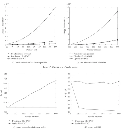
nodes, and “PSNR” indicates the data reconstruction qual-ity as detailed in the previous section. As we can see, along with the increasing of PSNR and distance, the performances of distributed algorithms are better than nondistributed ap-proach, and our proposed algorithm has the least energy con-sumption and delay. Notably, the shape ofFigure 2is not as regular as Figures3and4. This is because our algorithm can adjust the transform level adaptively according to the dis-tance, and thus the size of energy consumption, delay, and PSNR varies along with the transform level irregularly.
In Figure 5, we compare the performance of our pro-posed approach, 2-level WT, and nondistributed approach using energy × delay/PSNR metric.Figure 5(a) shows sce-nario when the cluster head is located at different positions.
Table1: The relations among optimal transforming level, distance, the reconstructed quality, energy, and delay.
Opt-level Distance (m) PSNR (dB) Energy (107nJ) Delay (104units)
1 20 61.1 0.8 5.3
2 30 58.4 1.0 3.6
3 40 56.8 1.3 3.2
3 50 56.6 1.6 3.2
4 60 55.4 2.0 3.1
4 70 55.4 2.4 3.1
4 80 55.4 2.8 3.1
4 90 55.4 3.4 3.1
4 100 55.4 3.9 3.1
4 110 55.4 4.6 3.1
4 120 55.4 5.3 3.1
4 130 55.4 6.0 3.1
5 140 55.4 6.9 3.1
5 150 55.4 7.8 3.1
5 160 55.4 8.8 3.1
5 170 55.4 9.7 3.1
5 180 55.4 11.0 3.1
5 190 55.4 11.9 3.1
5 200 55.4 13.1 3.1
when employing theenergy×delay/PSNRmetric. Our pro-posed algorithm also outperforms the general distributed al-gorithm.
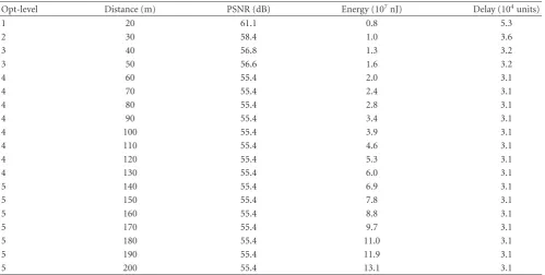
Figure 6shows the impact of border impact on data re-construction. Figure 6(a) indicates that the percentage of nodes, in which the reconstructed data is distortive out of the total 256 nodes, increases if the border effect is not removed along with the alteration of the wavelet function (From DB1 to DB7). Accordingly, the reconstructed data quality (PSNR) deteriorates as compared with our approach. InFigure 6(b), we intentionally employ threshold and quantization to form an application scenario where the compression is lossy. It shows that, even with lossy compression, in terms of data re-constructed quality, our approach far outperforms the tradi-tional distributed 2-level WT approach.
The relationship among optimal level of WT(Opt-level), distance between nodes and cluster head,PSNR, energy con-sumption, and delay is captured inTable 1. The result shows that the optimal transforming levels are different along with the variety of distance between nodes and cluster head while ensuring almost the same reconstructed quality. When the distance increases, the energy consumption increases and network delay decreases correspondingly. This is because en-ergy consumption is dependent on the distance under first-order radio model, and network delay only relies on the average number of encoding bits. In our simulation, when the proportion of the discarding detail coefficients to total wavelet coefficients in the WT reaches 73 percent, thePSNR
is still reach 49 dB. We believe that the reasons are the data used in the simulation have strong spatio-temporal correla-tions and our algorithm can move them efficiently.
As we can see from the simulation results, the optimal level of WT is 0 when the distance between nodes and
clus-ter head is less than 20 meclus-ters. This indicates that WT is not necessary under this case, and the non-distributed approach obtain good performance, for it has no additional energy consumption. However, with increasing distance between the nodes and the cluster head, the benefit of compression out-weigh the energy consumption due to inter-node commu-nication for performing the WT, and then the proposed al-gorithm will save more energy.Table 1shows that different transforming levels needed to be performed to obtain the similarPSNRwhile minimizing energy and delay cost.
5. CONCLUSION
In this paper, we have proposed a distributed optimal-level spatiotemporal compression algorithm based on the ring model for general wavelets with arbitrary supports. Our al-gorithm can accommodate a broad range of wavelet func-tions in order to effectively exploit the temporal and spa-tial correlation for data compression. Furthermore, the ring topology can effectively eliminate the “border effect” by nat-urally extending the signal space. In particular, our algorithm can choose optimal transforming levels to obtain better per-formance according to the given network circumstance. The proposedenergy×delay/PSNRmodel is capable of effectively evaluating the data compression algorithms for wireless sen-sor networks. The theoretical and experimental results show that the proposed scheme can achieve significant reduction in energy consumption and delay for data gathering in a sen-sor cluster.
ACKNOWLEDGMENT
This work is partially supported by the National High-Tech Research and Development Plan of China (863) under Grant no. 2006AA01Z227. Yonghe Liu is partially supported by US NSF Grant no. CNS-0721951 and Texas Advanced Research Program.
REFERENCES
[1] D. Estrin, R. Govindan, J. Heideman, and S. Kumar, “Next century challenges: scalable coordination in sensor networks,” inProceedings of the 5th ACM/IEEE International Conference on Mobile Computing and Networking (MOBICOM ’99), pp. 263–270, Seattle, Wash, USA, August 1999.
[2] S. Lindsey, C. Raghavendra, and K. M. Sivalingam, “Data gath-ering algorithms in sensor networks using energy metrics,”
IEEE Transactions on Parallel and Distributed Systems, vol. 13, no. 9, pp. 924–935, 2002.
[3] N. Xu, S. Rangwala, K. Chintalapudi, et al., “A wireless sen-sor network For structural monitoring,” inProceedings of the 2nd International Conference on Embedded Networked Sensor Systems, pp. 13–24, Baltimore, Md, USA, November 2004. [4] H. Chen, J. Li, and P. Mohapatra, “RACE: time series
compres-sion with rate adaptive and error bound for sensor networks,” inProceedings of the 1st IEEE International Conference on Mo-bile Ad-hoc and Sensor Systems (MASS ’0), pp. 124–133, Fort Lauderdale, Fla, USA, October 2004.
[5] D. Ganesan, D. Estrin, and J. Heidemann, “DIMENSIONS: why do we need a new data handling architecture for sensor networks?”Computer Communication Review, vol. 33, no. 1, pp. 143–148, 2003.
[6] D. Ganesan, D. Greenstein, D. Perelyubskiy, D. Estrin, and J. Heidemann, “An evaluation of multiresolution storage for sensor networks,” inProceedings of the 1st International Con-ference on Embedded Networked Sensor Systems (SenSys ’03), pp. 89–102, Los Angeles, Calif, USA, November 2003. [7] S. Servetto, “Distributed signal processing algorithms for the
sensor broadcast problem,” inProceedings of the 37th Annual Conference on Information Sciences and Systems (CISS ’03), Baltimore, Md, USA, March 2003.
[8] A. Ciancio and A. Ortega, “A dynamic programming approach to distortion-energy optimization for distributed wavelet compression with applications to data gathering in wireless sensor networks,” inProceedings of the IEEE International Con-ference on Acoustics, Speech and Signal Processing (ICASSP ’06), vol. 4, pp. 949–952, Toulouse, France, May 2006.
[9] R. S. Wagner, R. G. Baraniuk, S. Du, D. B. Johnson, and A. Co-hen, “An architecture for distributed wavelet analysis and pro-cessing in sensor networks,” inProceedings of the 5th Interna-tional Conference on Information Processing in Sensor Networks (IPSN ’06), pp. 243–250, Nashville, Tenn, USA, April 2006. [10] R. Cristescu, B. Beferull-Lozano, M. Vetterli, D. Ganesan, and
J. Acimovic, “On the interaction of data representation and routing in sensor networks,” inProceedings of IEEE Interna-tional Conference on Acoustics, Speech, and Signal Processing (ICASSP ’05), vol. 5, pp. 1109–1112, Philadelphia, Pa, USA, March 2005.
[11] I. Daubechies,Ten Lectures on Wavelets, SIAM, Philadelphia, Pa, USA, 1992.
[12] W. Heinzelman, A. Chandrakasan, and H. Balakrishnan, “Energy-efficient communication protocol for wireless mi-crosensor networks,” inProceedings of the 33rd Annual Hawaii
International Conference on System Sciences (HICSS ’00), vol. 8, p. 8020, Maui, Hawaii, USA, January 2000.