An Efficient Feature Extraction Method
with Pseudo-Zernike Moment in RBF
Neural Network-Based Human Face
Recognition System
Javad Haddadnia
Engineering Department, Tarbiat Moallem University of Sabzevar, Sabzevar, Khorasan 397, Iran Email:[email protected]
Majid Ahmadi
Electrical and Computer Engineering Department, University of Windsor, Windsor, Ontario, Canada N9B 3P4 Email:[email protected]
Karim Faez
Electrical Engineering Department, Amirkabir University of Technology, Tehran 15914, Iran Email:[email protected]
Received 17 April 2002 and in revised form 24 April 2003
This paper introduces a novel method for the recognition of human faces in digital images using a new feature extraction method that combines the global and local information in frontal view of facial images. Radial basis function (RBF) neural network with a hybrid learning algorithm (HLA) has been used as a classifier. The proposed feature extraction method includes human face localization derived from the shape information. An efficient distance measure as facial candidate threshold (FCT) is defined to distinguish between face and nonface images. Pseudo-Zernike moment invariant (PZMI) with an efficient method for selecting moment order has been used. A newly defined parameter named axis correction ratio (ACR) of images for disregarding irrelevant information of face images is introduced. In this paper, the effect of these parameters in disregarding irrelevant information in recognition rate improvement is studied. Also we evaluate the effect of orders of PZMI in recognition rate of the proposed technique as well as RBF neural network learning speed. Simulation results on the face database of Olivetti Research Laboratory (ORL) indicate that the proposed method for human face recognition yielded a recognition rate of 99.3%.
Keywords and phrases:human face recognition, face localization, moment invariant, pseudo-Zernike moment, RBF neural net-work, learning algorithm.
1. INTRODUCTION
Face recognition has been a very popular research topic in re-cent years because of wide variety of application domains in both academia and industry. This interest is motivated by ap-plications such as access control systems, model-based video coding, image and film processing, criminal identification and authentication in secure systems like computers or bank teller machines, and so forth [1]. A complete face recogni-tion system should include three stages. The first stage is de-tecting the location of the face, which is difficult because of unknown position, orientation, and scaling of the face in an arbitrary image [2,3,4]. The second stage involves extraction of pertinent features from the localized facial image obtained
in the first stage. Finally, the third stage requires classification of facial images based on the derived feature vector obtained in the previous stage.
eyes, nose, and mouth [6,7]. The structure-based approaches deal with local information instead of global information, and, therefore, they are not affected by irrelevant information in an image. However, because of the explicitness model of facial features, the structure-based approaches are sensitive to the unpredictability of face appearance and environmen-tal conditions [5]. The second method is a statistics-based approach that extracts features from the whole image and, therefore uses global information instead of local informa-tion. Since the global data of an image are used to determine the feature elements, information that is irrelevant to facial portion, such as hair, shoulders, and background, may cre-ate erroneous feature vectors that can affect the recognition results [8].
In recent years, many researchers have noticed this prob-lem and tried to exclude the irrelevant data while performing face recognition. This can be done by eliminating the irrele-vant data of a face image with a dark background [9] and constructing the face database under constrained conditions, such as asking people to wear dark jackets and to sit in front of a dark background [10]. Turk and Pentland [11] multi-plied the input image by a two-dimensional Gaussian win-dow centered on the face to diminish the effects caused by the nonface portion. Sung and Poggio [12] tried to eliminate the near-boundary pixels of a normalized face image by us-ing a fixed size mask. In [13], Liao et al. proposed a face-only database as the basis for face recognition.
In this paper, an efficient feature extraction technique is developed, based on the combination of local and global in-formation of face images. At first, face localization based on shape information [2,14] with a new definition for distance measure threshold called facial candidate threshold (FCT) for distinguishing between nonface image and facial image candidate is introduced. We present the effect of varying the FCT on the recognition rate of the proposed technique. A new parameter, called the axis correction ratio (ACR), is de-fined to eliminate irrelevant data from the face images and to create a subimage for further feature extraction. We have shown how ACR can improve the recognition rate. Once the face localization process is completed, pseudo-Zernike mo-ment invariant (PZMI) with a new method to select momo-ment orders is utilized to obtain the feature vector of the face un-der recognition. In this paper, PZMI was selected over other types of moments because of its utility in human face recog-nition approaches in [14,15]. The last step in human face recognition requires classification of the facial image into one of the known classes based on the derived feature vector ob-tained in the previous stage. The radial basis function (RBF) neural network is also used as the classifier [15, 16]. The training of the RBF neural network is done, based on the hy-brid learning algorithm (HLA) [17] and we have shown that the proposed feature extraction method with an RBF neural network classifier gives a faster training phase and yields a better recognition rate. The organization of this paper is as follows. Section 2presents the face localization method. In
Section 3, the face feature extraction is presented. Classifier
techniques are described inSection 4and finally, Sections5 and6present the experimental results and conclusions.
θ
Figure1: Face model based on ellipse model.
2. FACE LOCALIZATION METHOD
To ensure a robust and accurate feature extraction, the ex-act location of the face in an image is needed. The ultimate goal of the face localization is finding an object in an im-age as a face candidate whose shape resembles the shape of a face and, therefore, one of the key problems in building au-tomated systems that perform face recognition task is face localization. Many algorithms have been proposed for face localization and detection, which are based on using shape [2,4,14], color information [3], motion [18], and so forth. A critical survey on face localization and detection can be found in [5]. In this paper, we have used a modified version of the shape information technique for the face localization presented in [2,14].
Many researchers have concluded that an ellipse can gen-erally approximate the face of a human. The localization al-gorithm utilizes the information about the edges of the facial image or the region over which the face is located [3,14,15]. The advantage of the region-based method is its robustness in the presence of noise and changes in illumination. In the region-based method, the connected components are deter-mined by applying a region growing algorithm [3,14], then, for each connected component with a given minimum size, the best-fit ellipse is computed using the properties of the geometric moments. To find a face region, an ellipse model with five parameters is used:X0,Y0are the centers of the
el-lipse,θis the orientation, andαandβare the minor and the major axes of the ellipse, respectively, as shown inFigure 1. To calculate these parameters, first we review the geometric moments. The geometric moments of orderp+qof a digital image are defined as the digital image atxandylocation. The translation invari-ant central moments are obtained by placing origin at the center of the image
given by the center of gravity of the connected components. The orientation θ of the ellipse can be calculated by deter-mining the least moment of inertia [2,3,14]
where µpq denotes the central moment of the connected components as described in (2). The length of the major and the minor axes of the best-fit ellipse can also be computed by evaluating the moment of inertia. With the least and the greatest moments of inertia of an ellipse defined as
IMin=
the length of the major and the minor axes are calculated from [3,4,14] as
To assess how well the best-fit ellipse approximates the con-nected components, we define a distance measure between the connected components and the best-fit ellipse as follows:
φi=Pinside
µ00 , φo=
Poutside
µ00 , (6)
where thePinsideis the number of background points inside
the ellipse,Poutsideis the number of points of the connected
components that are outside the ellipse, andµ00is the size of
the connected components.
The connected components are closely approximated by their best-fit ellipses whenφiandφoare as small as possible. We have named the threshold values for φi andφo as FCT. Our experimental study indicates that when FCT is less than 0.1, the connected component is very similar to ellipse; there-fore it is a good candidate as a face region. Ifφiandφoare greater than 0.1, there is no face region in the input image, therefore, we reject it as a nonface image. An example of ap-plication of this method for locating face region candidates and rejecting nonface images has been presented inFigure 2.
3. FEATURE EXTRACTION TECHNIQUE
The aim of the feature extractor is to produce a feature vec-tor containing all pertinent information about the face while having a low dimensionality. In order to design a good face recognition system, the choice of feature extractor is very crucial. To design a system with low to moderate complex-ity, the feature vectors created from feature extraction stage should contain the most pertinent information about the face to be recognized. In the statistics-based feature extrac-tion approaches, global informaextrac-tion is used to create a set of
feature vector elements to perform recognition. A mixture of irrelevant data, which are usually part of a facial image, may result in an incorrect set of feature vector elements. There-fore, data that are irrelevant to facial portion such as hair, shoulders, and background should be disregarded in the fea-ture extraction phase.
Face recognition systems should be capable of recogniz-ing face appearances in a changrecogniz-ing environment. Therefore we use PZMI to generate the feature vector elements [14,15]. Also the feature extractor should create a feature vector with low dimensionality. The low-dimensional feature vector re-duces the computational burden of the recognition system; however, if the choice of the feature elements is not properly made, this in turn may affect the classification performance. Also, as the number of feature elements in the feature ex-traction step decreases, the neural network classifier becomes small with a simple structure. The proposed feature extractor in this paper yields a feature vector with low dimensionality, and, by disregarding irrelevant data from face portion of the image, it improves the recognition rate. The proposed feature extraction is done in two steps. In the first step, after face lo-calization, we create a subimage which contains information needed for the recognition algorithm. In the second step, the feature vector is obtained by calculating the PZMI of the de-rived subimage.
3.1. Creating a subimage
To create a subimage for feature extraction phase, all perti-nent information around the face region is enclosed in an ellipse while pixel values outside the ellipse are set to zero. Unfortunately, through creation of the subimage with the best-fit ellipse, as described inSection 2, many unwanted re-gions of the face image may still appear in this subimage, as shown inFigure 2. These include hair portion, neck, and part of the background as an example. To overcome this prob-lem, instead of using the best-fit ellipse for creating a subim-age, we have defined another ellipse. The proposed ellipse has the same orientation and center as the best-fit ellipse but the lengths of its major and minor axes are calculated from the lengths of the major and minor axes of the best-fit ellipse as follows:
A=ρ·α, B=ρ·β, (7)
whereAandBare the lengths of the major and minor axes of the proposed ellipse, andαandβare the lengths of the major and minor axes of the best-fit ellipse that have been defined in (5). The coefficientρis called ACR and varies from 0 to
1.Figure 3shows the effect of changing ACR whileFigure 4
shows the corresponding subimages.
φi=0.065 Figure2: Distinguishing between face and nonface using best-fit ellipse and FCT threshold.
ρ=1.0 ρ=0.7 ρ=0.4 Figure3: Different ellipses with respect to ACR.
Figure4: Subimage formation based on different ellipses and ACR values.
3.2. Pseudo-Zernike moment invariant
Statistics-based approaches for feature extraction are very important in pattern recognition for their computational ef-ficiency and their use of global information in an image for extracting features [15]. The advantages of considering or-thogonal moments are that they are shift, rotation, and scale invariants and are very robust in the presence of noise. The invariant properties of moments are utilized as pattern sen-sitive features in classification and recognition applications [14,19,20,21]. Pseudo-Zernike polynomials are well known and widely used in the analysis of optical systems. Pseudo-Zernike polynomials are orthogonal sets of complex-valued polynomials defined as (see [20,21])
Vnm(x, y)=Rnm(x, y) exp
The PZMI of ordernand repetitionmcan be computed us-ing the scale invariant central moments CMp,qand the radial geometric moments RMp,qas follows [21,22]:
PZMInm
3.3. Selecting feature vector elements
After face localization and subimage creation, we calculate the PZMI inside each subimage as face features. For select-ing the best order of the PZMI as face feature elements, we define a feature vector in face recognition application whose elements are based on the PZMI orders as follows:
Table1: Feature vector elements based on PZMI.
jvalue PZMI feature elements Number of feature elements nvalue Mvalue
3
3 0,1,2,3
60 4 0,1,2,3,4
5 0,1,2,3,4,5 6 0,1,2,3,4,5,6 7 0,1,2,3,4,5,6,7 8 0,1,2,3,4,5,6,7,8 9 0,1,2,3,4,5,6,7,8,9 10 0,1,2,3,4,5,6,7,8,9,10
6
6 0,1,2,3,4,5,6
45 7 0,1,2,3,4,5,6,7
8 0,1,2,3,4,5,6,7,8 9 0,1,2,3,4,5,6,7,8,9 10 0,1,2,3,4,5,6,7,8,9,10
9 9 0,1,2,3,4,5,6,7,8,9 21
10 0,1,2,3,4,5,6,7,8,9,10
jvalue
1 2 3 4 5 6 7 8 9
No.
o
f
m
o
m
en
ts
0 20 40 60 80
Figure5: Number of feature elements (PZMI) with respect toj.
4. CLASSIFIER DESIGN
Neural network is widely used as a classifier in many face recognition systems. Neural networks have been employed and compared to conventional classifiers for a number of classification problems. The results have shown that the ac-curacy of the neural network approaches is equivalent to, or slightly better than, other methods. Also, due to the simplic-ity, generalsimplic-ity, and good learning ability of the neural net-works, these types of classifiers are found to be more efficient [23].
RBF neural networks have been found to be very attrac-tive for many engineering problems because (1) they are uni-versal approximators, (2) they have a very compact topol-ogy, and (3) their learning speed is very fast because of their locally tuned neurons [16,17,23,24]. An important prop-erty of RBF neural networks is that they form a unifying link between many different research fields such as function approximation, regularization, noisy interpolation, and pat-tern recognition. Therefore, RBF neural networks serve as an
1
2
n
1
2
3
r
W11
Wrs
1
2
s
Figure6: RBF neural network structure.
excellent candidate for pattern classification where attempts have been carried out to make the learning process in this type of classification faster than normally required for the multilayer feedforward neural networks [23,25].
In this paper, an RBF neural network is used as a classifier in a face recognition system where the inputs to the neural network are feature vectors derived from the proposed fea-ture extraction technique described in the previous section.
4.1. RBF neural network structure
An RBF neural network structure is shown inFigure 6. The construction of the RBF neural network involves three dif-ferent layers with feedforward architecture. The input layer of the neural network is a set ofnunits, which accept the el-ements of ann-dimensional input feature vector. The input units are fully connected to the hidden layer withr hidden units. Connections between the input and hidden layers have unit weights and, as a result, do not have to be trained. The goal of the hidden layer is to cluster the data and reduce its di-mensionality. In this structure, the hidden units are referred to as the RBF units. The RBF units are also fully connected to the output layer. The output layer supplies the response of the neural network to the activation pattern applied to the input layer. The transformation from the input space to the RBF-unit space is nonlinear (nonlinear activation function), whereas the transformation from the RBF-unit space to the output space is linear (linear activation function). The RBF neural network is a class of neural networks where the acti-vation function of the hidden units is determined by the dis-tance between the input vector and a prototype vector. The activation function of the RBF units is expressed as follows [24,25]:
Ri(x)=Ri x−ci σi , i=
1,2, . . . , r, (14)
vectorσias follows:
Ri(x)=exp
−x−ci
2
σ2 i
. (15)
Note thatσi2represents the diagonal entries of the covariance matrix of the Gaussian function. The output units are linear and the response of the jth output unit for inputxis
yj(x)=b(j) + r
i=1
Ri(x)w2(i, j), (16)
wherew2(i, j) is the connection weight of theith RBF unit to
the jth output node andb(j) is the bias of the jth output. The bias is omitted in this network in order to reduce the neural network complexity [17,24,25]. Therefore,
yj(x)= r
i=1
Ri(x)×w2(i, j). (17)
4.2. RBF neural network classifier design
To design a classifier based on RBF neural networks, we have set the number of input nodes in the input layer of the neural network equal to the number of feature vector elements. The number of nodes in the output layer is then set to the number of image classes. The number of RBF units as well as their characteristic initialization is carried out using the following steps [17].
Step1. Initially, the RBF units are set equal to the number of outputs.
Step2. For each class k(k = 1,2, . . . , s), the center of the RBF unit is selected as the mean value of the sample features, belonging to the same class, that is,
Ck= Nk
i=1pk(n, i)
Nk , k=1,2, . . . , s, (18)
wherepk(n, i) is theith sample withnas the number of fea-tures belonging to classkandNkis the number of images in the same class.
Step3. For each classk, compute the distancedk from the meanCkto the farthest pointpk
f belonging to classk:
dk=pkf −Ck, k=1,2, . . . , s. (19)
Step4. For each classk, compute the distancedc(k, j) be-tween the mean of the class and the mean of other classes as follows:
dc(k, j)=Ck−Cj, j=1,2, . . . , s, j=k. (20)
Then, finddmin(k, l)=min(dc(k, j)) and check the
relation-ship betweendmin(k, l), dk, anddl. Ifdk+dl≤dmin(k, l), then
classkis not overlapping with other classes. Otherwise, class
kis overlapping with other classes and misclassifications may occur in this case.
Step5. If two classes are overlapped strongly, we first split one of the classes into two to remove the overlap. If the over-lap is not removed, the second class is also split. This requires addition of a new RBF unit to the hidden layer.
Step6. Repeat Steps2to5until all the training sample pat-terns are classified correctly.
Step7. The mean values of the classes are selected as the cen-ters of RBF units.
4.3. Hybrid learning algorithm
The training of the RBF neural networks can be made faster than the methods used to train multilayer neural networks. This is based on the properties of the RBF units, and can lead to a two-stage training procedure. The first stage of the train-ing involves determintrain-ing output connection weights, which requires solution of a set of linear equations which can be done fast. In the second stage, the parameters governing the basis function (corresponding to the RBF units) are deter-mined using an unsupervised learning method that requires solution of a set of nonlinear equations. The training of the RBF neural networks involves estimating output connection weights, centers, and widths of the RBF units. Dimension-ality of the input vector, and the number of classes set the number of input and output units, respectively. In this pa-per, an HLA, which combines the gradient method and the linear least square (LLS) method, is used for training the neu-ral network [17]. This is done in two steps. In the first step, the neural network connection weights in the output of the RBF units (w2(i, j)) are adjusted under the assumption that
the centers and the widths of the RBF units are known a pri-ori. In the second step, the centers and widths (candσ) of the RBF units are updated as described later.
4.3.1. Computing connection weights
Let r and s be the number of inputs and outputs, re-spectively, and assume that the number of u RBF outputs is generated for all training face patterns. For any input Pi(p1i, p2i, . . . , pri), the jth outputyjof the RBF neural net-work in (14) can be calculated in a more compact form as follows:
W2×R=Y, (21)
whereR∈ u×N is the matrix of the RBF units,W
2∈ s×u
is the output connection weight matrix, Y ∈ s×N is the output matrix, andNis the total number of sample face pat-terns. The relationship for error is defined by
E= T−Y, (22)
one nonzero element and identifies the processing pattern to which the given exemplar belongs.
Our objective is to find an optimal coefficient matrix W2∈ s×usuch thatETEis minimized. This is done by the
well-known LLS method [16] as follows:
W2×R=Y. (23)
The optimalW2is given by
W2=T×R+, (24)
whereR+is the pseudoinverse ofRand is given by
R+=RTR−1RT. (25)
We can compute the connection weights using (22) and (23) by knowing matrixRas follows:
W2=T
RTR−1RT. (26)
4.3.2. Defining the center and width of the RBF units Here, the center and width of the RBF units (Rmatrix) are adjusted by taking the negative gradient of the error function, En, for thenth sample pattern which is given by [25]
whereyknandtnkrepresent thekth real output and target out-put of thenth sample face pattern, respectively.
For the RBF units with the centerCand the widthσ, the update value for the center can be derived from (25) by the chain rule as follows:
and the update value for the width is computed as follows:
∆σn able of thenth sample face pattern, andξis the learning rate. ∆Cn(i, j) is the update value for theith variable of the center of the jth RBF unit based on thenth training pattern.∆σnj is the update value for the width of the jth RBF unit with respect to thenth training pattern.
Figure7: Samples of facial images in ORL database.
5. EXPERIMENTAL RESULTS
To check the utility of our proposed algorithm, experimental studies are carried out on the ORL database images of Cam-bridge University. This database contains 400 facial images from 40 individuals in different states, taken between April 1992 and April 1994. The total number of images for each person is 10. None of the 10 images is identical to any other. They vary in position, rotation, scale, and expression. The changes in orientation have been accomplished by each per-son rotating a maximum of 20 degrees in the same plane, as well as each person changing his/her facial expression in each of the 10 images (e.g., open/close eyes, smiling/not smil-ing). The changes in scale have been achieved by changing the distance between the person and the video camera. For some individuals, the images were taken at different times and varying facial details (glasses/no glasses). All the images were taken against a dark homogeneous background. Each image was digitized and presented by a 112×92 pixel ar-ray whose gar-ray levels ranged between 0 and 255. Samples of database used are shown inFigure 7.
jvalue
1 2 3 4 5 6 7 8 9
Er
ro
r
rat
e
(%)
1.2 1.25 1.3 1.35 1.4
Figure8: Error rate with respect toj.
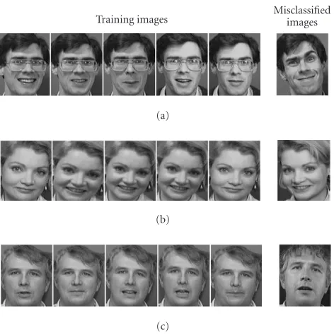
Training images Misclassifiedimages
(a)
(b)
(c)
Figure9: Misclassified images with corresponding training images.
5.1. Effect of moment orders
In this phase of the experiment, simulation has been done, based on the j value defined in (13). The ACR has been set equal to one and the RBF neural network classifier has been trained for each j value based on the training images.
Figure 8shows the error rate of the system with respect to
j. This figure shows that when jincreases, the error rate al-most remains unchanged. In contrast, asFigure 5has shown, when jincreases, the number of feature elements of the fea-ture vector in the feafea-ture extraction step decreases. This ob-servation is interesting because in spite of the decrease in the number of feature elements, the error rate has remained un-changed. Also, these results show that higher orders of the PZMI contain more and useful information for face recog-nition process.Figure 9shows the misclassified images and their corresponding training sets for the value of j =9. As indicated inFigure 9a, the misclassified image in this set is
ACR value
0
.
4
0
.
45 50. 0.55 06. 0.65 0.7 750. 0.8 0.85 0.9 0.95 1
Er
ro
r
rat
e
(%)
0 2 4 6 8 10
Figure10: Error rate variation with respect to ACR value.
substantially different from the training set in terms of its fa-cial expression, while the reason for misclassification of the images in Figures9band9ccan be explained with the effect of the irrelevant data in the test images with respect to their training sets.
5.2. Effect of ACR when disregarding irrelevant data For the purpose of evaluating how the irrelevant data of a fa-cial image such as hair, neck, shoulders, and background will influence the recognition results, we have chosen the PZMI of orders 9 and 10 (set j=9) for feature extraction. We have also selected FCT= 0.1 for the face localization algorithm and the RBF neural network with the HLA as the classifier. We varied the ACR value and evaluated the recognition rate of the proposed algorithm.Figure 10shows the effect of ACR values on the error rate.
AsFigure 10shows, the error rate varies as the ACR
val-ues change. At ACR=1, a recognition rate of 98.7% is ob-tained (Section 5.1). Now, by changing ACR and calculating the correct recognition rate, it is observed that at ACR=0.87, a recognition rate of 99.3% can be achieved. This clearly in-dicates the importance of the ACR in improving the recogni-tion performance.
5.3. Effect of FCT when distinguishing between face and nonface regions
To evaluate the effect of FCT in the face localization step and distinguishing between face and nonface images, we pre-pared 20 nonface images and applied them to the system.
Figure 2shows a sample of such images withφi =0.13 and
φo=0.191. We varied the FCT value and evaluated the num-ber of nonface images that passed through the system. Exper-imental results showed that FCT=0.1 is a good threshold for distinguishing between face and nonface images. Figure 11 shows this result.
FCT value
as feature vector elements. The number of the feature vec-tor elements in this category is 27. In the second category, n = 4,5,6,7 is chosen. All the moments of each order in-cluded in this category are summed up to create a feature vector of size 26. In the third category, n = 6,7,8 is con-sidered, and the feature vector has 24 elements. Finally, in the last category, n = 9,10 is considered with 21 feature elements. The neural network classifier was trained in each category based on the training images, and subsequently, the system was tested using the test images. The experimen-tal results are shown inTable 2. This table indicates that in the training phase of the RBF neural network classifier, the number of epochs decreases when the PZMI orders increase. On the other hand, the RBF neural network with the HLA learning method has converged faster in the training phase when higher orders of the PZMI are used in comparison with the lower orders of PZMI. Also, this table indicates that the HLA method in the training phase has a lower root mean squared error (RMSE) with a good discrimination capabil-ity.
To compare the HLA with other learning algorithms, we have developed the k-mean clustering algorithm for train-ing the RBF neural networks [17,26] and applied it to the database with the same feature extraction technique.Table 3 shows the comparison between the two learning methods. It is seen fromTable 3that the HLA method converges faster than thek-mean clustering which needs fewer epochs in the training phase. Also, the RMSE during the training phase for the HLA is smaller than that for thek-mean clustering learn-ing algorithm.
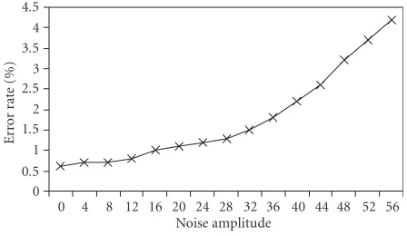
5.5. Performance evaluation in the presence of noise To evaluate the performance of the feature extraction method with ACR parameter, PZMI, and the RBF neural net-work for human face recognition in the presence of noise, a white Gaussian noise of zero mean and different amplitudes (in gray-level image) has been added to the clean images. The recognition process was then applied to the noisy images.
Figure 12shows the error rate of the recognition process with
respect to different values of the noise amplitude. This figure indicates that the proposed technique for human face
recog-Noise amplitude
Figure12: Error rate with respect to noise amplitude.
nition is very robust in the presence of noise. InFigure 13, samples of noisy images have been shown.
5.6. Comparison with other human face recognition systems
To compare the effectiveness of the proposed method with other algorithms, the PZMI of orders 9 and 10 with 21 feature elements, FCT=0.1, ACR=0.87, and the RBF neural net-work with the HLA learning algorithm have been used. This study compares the proposed technique with the methods that used the same ORL database. These include the shape information neural network (SINN) [15], convolution neu-ral network (CNN) [27], nearest feature line (NFL) [28], and the fractal transformation (FT) [29]. In this comparison, the training set and the test set were derived in the same way as was suggested in [15,27,28,29]: the 10 images from each class of the 40 persons were randomly partitioned into sets, resulting in 200 training images and 200 test images, with no overlap between the two. Also in this study, the error rate was defined, as was used in [15,27,28,29], to be the number of misclassified images in the test phase over the total number of test images. To conduct the comparison, an average error rate which has been used in [15,27,28,29] was utilized as
wheremis the number of experimental runs, each being per-formed on a random partitioning of the database into sets, Ni
mis the number of misclassified images for theith run, and Nt is the number of total test images for each run.Table 4 shows the comparison between the different techniques us-ing the same ORL database in terms of Eave. In this table,
Table2: Effect of the HLA method in learning phase.
Features vectors Training phase Testing phase
Category No. of feature flements No. of epochs RMSE No. of misclassified Error rate
n=1,2, . . . ,6 27 80∼100 0.09∼0.06 15 7.5%
n=4,5,6,7 26 60∼80 0.06∼0.04 9 4.5%
n=6,7,8 24 45∼60 0.04∼0.02 6 3%
n=9,10 21 30∼45 0.04∼0.01 3 1.3%
Table3: Comparison between the two learning techniques.
Feature category K-mean clustering HLA method
No. of epochs RMSE No. of epochs RMSE
n=1,2, . . . ,6 135∼120 0.12∼0.09 80∼100 0.09∼0.06
n=4,5,6,7 120∼95 0.09∼0.06 60∼80 0.06∼0.04
n=6,7,8 95∼70 0.06∼0.04 45∼60 0.04∼0.02
n=9,10 70∼50 0.04∼0.02 30∼45 0.04∼0.01
Noise amplitude=10
Noise amplitude=20
Noise amplitude=40
Noise amplitude=50
Figure13: Samples of noisy images with different noise value.
6. CONCLUSIONS
This paper presented an efficient method for the recognition of human faces in frontal view of facial images. The pro-posed technique utilizes a modified feature extraction tech-nique, which is based on a flexible face localization algorithm followed by PZMI. An RBF neural network with the HLA method was used as a classifier in this recognition system.
Table4: Error rates of different approaches.
Methods experimental (No. of Eave%
m)
CNN [27] 3 3.83
NFL [28] 4 3.125
FT [29] 1 1.75
SINN [15] 4 1.323
Proposed method 3 0.682
The paper introduces several parameters for efficient and ro-bust feature extraction technique as well as the RBF neural network learning algorithm. These include FCT, ACR, and selection of the PZMI orders and the HLA method. Exhaus-tive experimentation was carried out to investigate the effect of varying these parameters on the recognition rate. We have shown that high order PZMI contains very useful informa-tion about the facial images, and that the HLA method affects the learning speed. We have also indicated the optimum val-ues of the FCT and ACR corresponding to the best recogni-tion results on the ORL database. The robustness of the pro-posed algorithm in the presence of noise is also investigated. The highest recognition rate of 99.3% with ORL database was obtained using the proposed algorithm. We have imple-mented and tested some of the existing face recognition tech-niques on the same ORL database. This comparative study indicates the usefulness and the utility of the proposed tech-nique.
ACKNOWLEDGMENTS
REFERENCES
[1] M. A. Grudin, “On internal representation in face recognition systems,” Pattern Recognition, vol. 33, no. 7, pp. 1161–1177, 2000.
[2] J. Haddadnia and K. Faez, “Human face recognition using shape information and pseudo Zernike moments,” inProc. 5th International Fall Workshop Vision, Modeling and Visu-alization (VMV ’00), pp. 113–118, Saarbr¨ucken, Germany, November 2000.
[3] K. Sobottka and I. Pitas, “Face localization and facial feature extraction based on shape and color information,” inProc. IEEE International Conference on Image Processing (ICIP ’96), vol. 3, pp. 483–486, Lausanne, Switzerland, September 1996. [4] J. Wang and T. Tan, “A new face detection method based on
shape information,” Pattern Recognition Letter, vol. 21, no. 6-7, pp. 463–471, 2000.
[5] E. Hjelmas and B. K. Low, “Face detection: a survey,” Com-puter Vision And Image Understanding, vol. 83, no. 3, pp. 236– 274, 2001.
[6] M. Bichsel and A. P. Pentland, “Human face recognition and the face image sets topology,” CVGIP: Image Understanding, vol. 59, no. 2, pp. 254–261, 1994.
[7] V. Bruce, P. J. B. Hancock, and A. M. Burton, “Comparisons between human and computer recognition of faces,” inProc. 3rd International Conference On Automatic Face and Gesture Recognition (FG ’98), pp. 408–413, Nara, Japan, April 1998. [8] L.-F. Chen, H.-Y. M. Liao, J.-C. Lin, and C.-C. Han, “Why
recognition in a statistics-based face recognition system should be based on the pure face portion: a probabilistic decision-based proof,” Pattern Recognition, vol. 34, no. 7, pp. 1393–1403, 2001.
[9] P. N. Belhumeur, J. P. Hespanha, and D. J. Kriegman, “Eigen-faces vs. fisher“Eigen-faces: recognition using class specific linear pro-jection,” IEEE Trans. on Pattern Analysis and Machine Intelli-gence, vol. 19, no. 7, pp. 711–720, 1997.
[10] F. Goudail, E. Lange, T. Iwamoto, K. Kyuma, and N. Otsu, “Face recognition system using local autocorrelations and multiscale integration,” IEEE Trans. on Pattern Analysis and Machine Intelligence, vol. 18, no. 10, pp. 1024–1028, 1996. [11] M. Turk and A. Pentland, “Eigenfaces for recognition,”
Jour-nal of Cognitive Neuroscience, vol. 3, no. 1, pp. 71–86, 1991. [12] K. K. Sung and T. Poggio, Example-Based Learning for
View-Based Human Face Detection, vol. 1521 ofA.I. Memo, MIT Press, Cambridge, Mass, USA, 1994.
[13] H.-Y. M. Liao, C.-C. Han, and G.-J. Yu, “face + hair + shoulders + background = face,” inProc. Workshop on 3D Computer Vision ’97, pp. 91–96, The Chinese University of Hong Kong, Hong Kong, China, May 1997.
[14] J. Haddadnia, M. Ahmadi, and K. Faez, “An efficient method for recognition of human faces using higher orders pseudo Zernike moment invariant,” inProc. 5th International Confer-ence On Automatic Face and Gesture Recognition (FG ’02), pp. 330–335, Washington, DC, USA, May 2002.
[15] J. Haddadnia, K. Faez, and P. Moallem, “Neural network based face recognition with moments invariant,” inProc. IEEE International Conference on Image Processing (ICIP ’01), vol. 1, pp. 1018–1021, Thessaloniki, Greece, October 2001.
[16] J. Haddadnia and K. Faez, “Human face recognition using ra-dial basis function neural network,” inProc. 3rd International Conference On Human and Computer (HC ’00), pp. 137–142, Aizu, Japan, September 2000.
[17] J. Haddadnia, M. Ahmadi, and K. Faez, “A hybrid learning RBF neural network for human face recognition with pseudo Zernike moment invariant,” inIEEE International Joint
Con-ference On Neural Network (IJCNN ’02), pp. 11–16, Honolulu, Hawaii, USA, May 2002.
[18] R. Herpers, G. Verghese, K. Derpanis, et al., “Detection and tracking of faces in real environments,” in IEEE Interna-tional Workshop on Recognition, Analysis, and Tracking of Face and Gesture in Real-Time Systems, pp. 96–104, Corfu, Greece, September 1999.
[19] S. X. Liao and M. Pawlak, “On the accuracy of Zernike mo-ments for image analysis,”IEEE Trans. on Pattern Analysis and Machine Intelligence, vol. 20, no. 12, pp. 1358–1364, 1998. [20] C. H. Teh and R. T. Chin, “On image analysis by the methods
of moments,” IEEE Trans. on Pattern Analysis and Machine Intelligence, vol. 10, no. 4, pp. 496–513, 1988.
[21] S. O. Belkasim, M. Shridhar, and M. Ahmadi, “Pattern recog-nition with moment invariants: a comparative study and new results,” Pattern Recognition, vol. 24, no. 12, pp. 1117–1138, 1991.
[22] R. R. Bailey and M. Srinath, “Orthogonal moment features for use with parametric and non-parametric classifiers,”IEEE Trans. on Pattern Analysis and Machine Intelligence, vol. 18, no. 4, pp. 389–399, 1996.
[23] W. Zhou, “Verification of the nonparametric characteristics of backpropagation neural networks for image classification,”
IEEE Transactions on Geoscience and Remote Sensing, vol. 37, no. 2, pp. 771–779, 1999.
[24] L. Yingwei, N. Sundararajan, and P. Saratchandran, “Perfor-mance evaluation of a sequential minimal radial basis func-tion (RBF) neural network learning algorithm,” IEEE Trans-actions on Neural Networks, vol. 9, no. 2, pp. 308–318, 1998. [25] J.-S. R. Jang, “ANFIS: adaptive-network-based fuzzy inference
system,” IEEE Trans. Systems, Man, and Cybernetics, vol. 23, no. 3, pp. 665–685, 1993.
[26] S. Gutta, J. R. J. Huang, P. Jonathon, and H. Wechsler, “Mix-ture of experts for classification of gender, ethnic origin, and pose of human faces,”IEEE Transactions on Neural Networks, vol. 11, no. 4, pp. 948–960, 2000.
[27] S. Lawrence, C. L. Giles, A. C. Tsoi, and A. D. Back, “Face recognition: a convolutional neural network approach,”IEEE Transactions on Neural Networks, vol. 8, no. 1, pp. 98–113, 1997.
[28] S. Z. Li and J. Lu, “Face recognition using the nearest feature line method,” IEEE Transactions on Neural Networks, vol. 10, no. 2, pp. 439–443, 1999.
[29] T. Tan and H. Yan, “Face recognition by fractal transforma-tions,” inProc. IEEE Int. Conf. Acoustics, Speech, Signal Pro-cessing (ICASSP ’99), vol. 6, pp. 3537–3540, Phoenix, Ariz, USA, March 1999.
Javad Haddadniareceived his B.S. and M.S. degrees in electrical and electronic engi-neering with the first rank from Amirk-abir University of Technology, Tehran, Iran, in 1993 and 1995, respectively. He received his Ph.D. degree in electrical engineering from Amirkabir University of Technology, Tehran, Iran in 2002. He joined Tarbiat Moallem University of Sabzevar in Iran. His research interests include neural network,
Majid Ahmadireceived his B.S. in electri-cal engineering from Arya-Mehr University and Ph.D. degree in electrical engineering from Imperial College of London Univer-sity in 1971 and 1977, respectively. Dr. Ah-madi has been a Professor in the Depart-ment of Electrical and Computer Engineer-ing, University of Windsor since 1980. Dr. Ahmadi has conducted research in the areas of 2D signal processing, image processing
and computer vision, pattern recognition, neural network archi-tectures, applications and VLSI realization, computer arithmetic, and MEMS. He has published over 300 papers in these areas. He is a Fellow of the IEEE (USA) and a Fellow of the IEE (UK).
Karim Faezwas born in Semnan, Iran. He received his B.S. degree in electrical engi-neering from Tehran Polytechnic University with the first rank in June 1973, and his M.S. and Ph.D. degrees in computer science from University of California at Los Ange-les (UCLA) in 1977 and 1980, respectively. Professor Faez was with Iran Telecommuni-cation Research Center (1981–1983) before joining Amirkabir University of Technology