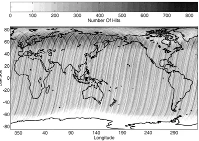
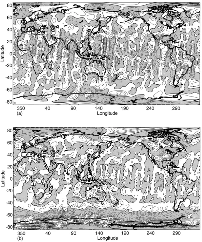
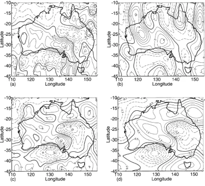
Ørsted and Magsat scalar anomaly fields

Earth Planets Space, 52, 1207?1211, 2000 An estimate of the errors of the IGRF/DGRF fields 1945?2000 F J Lowes Physics Department, University of Newcastle, Newcastle upon Tyne, NE1 7RU, U

Earth Planets Space, 54, 231?237, 2002 Self potential anomaly of Satsuma Iwojima volcano Wataru Kanda and Sin?yo Mori Sakurajima Volcano Research Center, Disaster Prevention

Earth Planets Space, 54, 907?916, 2002 Unusual ionospheric absorption characterizing energetic electron precipitation into the South Atlantic Magnetic Anomaly Masanori Nishino1,

Sato et al Earth, Planets and Space 2014, 66 68 http //www earth planets space com/content/66/1/68 LETTER Open Access Detailed bathymetry and magnetic anomaly in the Central Ryukyu Arc,

Earth Planets Space, 57, 385?392, 2005 Simultaneous ground and satellite based airglow observations of geomagnetic conjugate plasma bubbles in the equatorial anomaly Tadahiko Ogawa1,

Earth Planets Space, 58, 607?616, 2006 Energetic particle precipitation in the Brazilian geomagnetic anomaly during the ?Bastille Day storm? of July 2000 Masanori Nishino1?, Kazuo

Earth Planets Space, 63, 371?375, 2011 Weakening of the mid latitude summer nighttime anomaly during geomagnetic storms Huixin Liu1,2 and Mamoru Yamamoto3 1Earth and Planetary

Earth Planets Space, 59, 401?405, 2007 Variations in the equatorial ionization anomaly peaks in the Western Pacific region during the geomagnetic storms of April 6 and July 15, 2000