Open Access
Proceedings
Efficient detection of QTL with large effects in a simulated pig-type
pedigree using selective genotyping
Henri CM Heuven*
1,2, John WM Bastiaansen
2and Stéphanie M van
den Berg
1Address: 1Clinical Sciences of Companion Animals, Faculty of Veterinary Medicine, Utrecht University. P.O. box 80163, 3508 TD Utrecht, The
Netherlands and 2Animal Breeding and Genomics Centre, Wageningen University, P.O.-box 338, 6700AH Wageningen, the Netherlands
Email: Henri CM Heuven* - [email protected]; John WM Bastiaansen - [email protected]; Stéphanie M van den Berg - [email protected]
* Corresponding author
Abstract
Background: The ultimate goal of QTL studies is to find causative mutations, which requires additional expression studies. Given the limited amount of time and funds, the smart option is to identify the most important QTL with minimal effort. A cost-effective solution is to genotype only those animals with high or low phenotypic values or DNA-pools of these individuals. A two-stage genotyping strategy was applied on samples in the tails of the distribution of breeding values.
Results: The tail-analysis approach identified eight out of the 19 QTL in the first stage, explaining about half of 98% of the genetic variance. Four additional QTL with small effects were found in the second stage.
Conclusion: The two-stage genotyping strategy with selective genotyping detected regions with highly significant QTL useful for further fine-mapping. The large reduction in costs allows for follow-up expression and functional studies.
Background
Discovery and subsequent validation of causative muta-tions affecting complex traits require identification and fine-mapping of QTL followed by expression and func-tional studies. Given the limited amount of time and funds, the challenge is to identify the most important QTL with minimal effort.
A cost-effective strategy is to reduce genotyping costs by only genotyping individuals with high and low pheno-typic values, or to genotype pools of these individuals. Tail analysis, bulked segregant analysis and selective DNA pooling have been advocated by Hillel et al. [1], Michel-more et al. [2] and Darvasi and Soller [3]. More recently Korol et al. [4] improved on the latter method by studying fractioned DNA pooling. Disadvantages to genotyping tails or pools are the number of traits that can be studied
from 12th European workshop on QTL mapping and marker assisted selection Uppsala, Sweden. 15–16 May 2008
Published: 23 February 2009
BMC Proceedings 2009, 3(Suppl 1):S8
<supplement> <title> <p>Proceedings of the 12th European workshop on QTL mapping and marker assisted selection</p> </title> <sponsor> <note>Publication of this supplement was supported by EADGENE (European Animal Disease Genomics Network of Excellence).</note> </sponsor> <note>Proceedings</note> <url>http://www.biomedcentral.com/content/pdf/1753-6561-3-S1-info.pdf</url> </supplement> This article is available from: http://www.biomedcentral.com/1753-6561/3/S1/S8
© 2009 Heuven et al; licensee BioMed Central Ltd.
with the selected genotypes, separate high/low tails or pools have to be made for each trait, and non-optimal use of haplotype information. Wang et al. [5] improved on statistical methods developed by Dekkers [6] for interpre-tation of results obtained by DNA pooling.
Commercial breeding pedigrees present a situation where phenotypes are abundant, across many generations. In such a situation, selective genotyping is an important step in setting up a cost effective QTL study. This study imple-ments a two-stage strategy. First, genotypes on a large SNP panel are obtained for highly informative individuals, that is, individuals with extreme breeding values. High and low phenotype animals are selected within each sire-dam pairing in order to control for stratification.
The objective is to identify major segregating QTL in a simulated pig-type pedigree with minimal effort both in terms of genotyping and analysis.
Methods
In a four generation pedigree, 45 sires produced 100 off-spring each. Each sire was mated to 10 dams with 10 prog-eny each. Sires and dams of the base generation were unknown. All 4665 animals were phenotyped for a quan-titative trait (TRT). Six thousand equally distributed (0.1 cM) SNPs were available for genotyping, located on 6 chromosomes of 100 cM each. A full description of the dataset can be found at the website of XIIth QTLmas work-shop [7].
Genotyping strategy
Stage 1
For each sire, the offspring with the highest and the lowest EBV within a set of full sibs (i.e. per dam) were included into the high tail (H-tail) and the low tail (L-tail) respec-tively. Since there were 10 dams per sire there were 10 ani-mals in either tail for each sire. Only sires with progeny that have phenotype records were used.
For each SNP and for each sire, the frequencies of the '1' and '2'-alleles in the high and low tail were determined and submitted to a χ2 (1) test. SNPs with a Pearson statis-tic exceeding 10 (nominal p-value < 0.0016) were consid-ered putative. A Pearson χ2 value exceeding 10 required that the counts of the allele in either tail differed by at least 10. A difference of 10 alleles suggested linkage between a QTL and this SNP in the sire, assuming equal contribu-tions of the dam's alleles to both tails. A Chi-square test was appropriate under the null hypothesis of no associa-tion and the assumpassocia-tion that both sires and dams were sampled randomly from the population with respect to their SNP genotypes.
Stage 2
When multiple segregating SNPs occur in a small region then this region was considered likely to contain a QTL. Genotypes of all putative SNPs were subsequently obtained for all animals with phenotype records and an association was determined by applying the following model:
TRT = μ + Zu + SNP + e (1)
Where:
TRT = trait value
μ = overall mean
Z = incidence matrix linking polygenic effects to individu-als
u = polygenic effect ~N(0, Aσa2) with A as the additive genetic relationship matrix
SNP = effect of single SNP (four classes: 11, 12, 21, 22)
e = residual effects ~N(0, Iσe2); with I as the Identity matrix
Model selection, i.e. which SNP(s) needs be included in the model, was determined by region. Forward stepwise regression was applied to identify markers with a large effect.
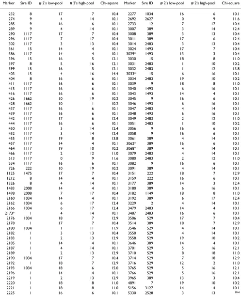
Table 1: Putative markers identified using Chi-square tests on high and low tails for each sire.
Marker Sire ID # 2's low-pool # 2's high-pool Chi-square Marker Sire ID # 2's low-pool # 2's high-pool Chi-square
232 8 17 7 10.4 2277 1034 16 6 10.1
274 9 4 14 10.1 2692 2627 0 9 11.6
285 9 16 6 10.1 2733 12 7 17 10.4
289 9 4 14 10.1 3007 389 3 14 12.4
290 1117 17 7 10.4 3008 389 3 13 10.4
296 1117 7 17 10.4 3011 389 17 6 12.4
302 1117 3 13 10.4 3014 2483 3 13 10.4
361 15 14 4 10.1 3024 1493 17 7 10.4
386 1117 14 4 10.1 3029* 1493 13 3 10.4
396 15 16 5 12.1 3030 15 18 8 11.0
397 8 5 16 12.1 3031 2483 1 10 10.2
399 15 16 5 12.1 3032 2483 1 12 13.8
403 15 4 16 14.4 3033* 15 6 16 10.1
404 8 16 6 10.1 3034 2483 19 10 10.2
411 1117 16 6 10.1 3039 9 18 8 11.0
415 1117 16 6 10.1 3040 1493 6 16 10.1
416 1117 16 6 10.1 3043 1493 14 4 10.1
426 1662 10 19 10.2 3045 9 16 6 10.1
428 1662 10 1 10.2 3046 1493 6 16 10.1
437 1117 16 6 10.1 3047 2483 4 14 10.1
439 1117 16 6 10.1 3048 1493 6 16 10.1
442 1117 17 6 12.4 3049 2483 2 12 11.0
444 1117 16 6 10.1 3051 2483 1 10 10.2
450 1117 3 14 12.4 3056 9 16 6 10.1
452 1117 3 14 12.4 3058 9 16 6 10.1
455 1117 19 8 13.8 3061 389 4 14 10.1
457 1117 14 4 10.1 3062* 389 16 6 10.1
464 1117 19 10 10.2 3068* 389 4 14 10.1
466 1117 2 12 11.0 3079 2483 4 14 10.1
513 1117 0 9 11.6 3080 2483 2 12 11.0
534 1117 16 6 10.1 3082 9 16 6 10.1
726 222 10 19 10.2 3091 389 4 14 10.1
1125 1475 17 7 10.4 3151 222 18 7 12.9
1212 8 14 4 10.1 3159 222 16 6 10.1
1326 8 4 14 10.1 3177 389 14 3 12.4
1483 2008 14 4 10.1 3180 389 6 16 10.1
1498 2008 7 17 10.4 3182 1149 18 8 11.0
2160 1034 14 4 10.1 3192 389 6 17 12.4
2162 1034 6 17 12.4 3229 2 4 14 10.1
2166 1034 6 17 12.4 3479 2483 14 4 10.1
2173* 1 4 14 10.1 3487 2483 16 6 10.1
2176 1034 18 7 12.9 3506 529 17 7 10.4
2178 1 17 7 10.4 3514 389 18 7 12.9
2180 1034 1 11 11.9 3546 529 4 14 10.1
2182 1 3 13 10.4 3550 529 4 14 10.1
2183 1 2 13 12.9 3558 529 19 10 10.2
2185 1 14 4 10.1 3646 389 14 4 10.1
2187 1 4 14 10.1 3701 529 5 16 12.1
2189 1 2 13 12.9 3710 529 8 18 11.0
2190 1034 17 7 10.4 3714 529 7 18 12.9
2192 1 18 7 12.9 3716 529 12 2 11.0
2193 1034 18 6 15.0 3765 529 5 16 12.1
2196 1 14 4 10.1 3766 529 5 16 12.1
2219 1 2 13 12.9 3965 389 13 3 10.4
2220 1 18 8 11.0 4891 7 19 10 10.2
2221 1 18 8 11.0 5156 3127 14 4 10.1
2225 1 16 6 10.1 5330 2528 3 13 10.4
Results
Stage 1114 putative markers significantly (p < 0.0016) differed in frequency between the high and low tail in at least one sire family (Table 1). Five markers were significantly different between tails in 2 sire families, but all other putative markers were discovered from the difference between pools in only a single sire family. The putative markers were identified in tails from 21 sires of which 8 sires seg-regated only for one putative marker. In 24 sire families no SNPs were identified as putative. Most of the 114 puta-tive markers occurred in groups of positions, indicating regions where QTL might be segregating.
Stage 2
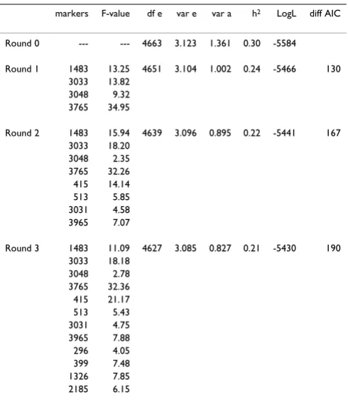
The next step was to obtain genotypes for all phenotyped animals for the putative markers identified in stage 1, in order to distinguish between truly associated markers and false positives. Individual marker association with the trait was calculated using model 1 (i.e. a model including each marker in turn as well as a polygenic effect). Table 2 summarizes these results. Table 3 shows the results of for-ward stepwise regression. In each subsequent analysis four SNPs with the most significant associations (F-statis-tics obtained after correcting for the previous entered SNPs) were added. The polygenic variance decreased indi-cating that 12 markers accounted for close to 30% of the genetic variance. The results of the third round indicate that on each of chromosomes 1, 2 and 4 there were regions with QTL. The size of the QTL can be deduced from the effects of the genotypes in round three (Table 4). With 100 progeny per sire, haplotypes could easily be determined and genotypes 12 and 21 could be distin-guished in most cases. QTL with the largest effects are expected near SNP 415, 3033 and 3765. Except for SNP 513, heterozygous genotype effects were intermediate to the effects of the homozygous genotypes indicating that the QTL were additive.
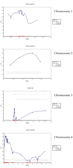
Subsequently LDLA was applied to these 114 markers and the profiles of the likelihood ratio test are shown in Figure 1 for chromosomes 1, 2, 3, and 4. Given these graphs and results from Table 3, two QTL are expected on chromo-some 1, one QTL on chromochromo-some 2, three or four QTL on chromosome 4 and none on chromosomes 3, 5, and 6.
Two very obvious candidates for further study were the regions between SNP 403 and SNP 466 on chromosome 1 and between SNP 3007 and SNP 3091 on chromosome 4. Both regions had a maximum log likelihood ratio greater than 80. QTLs with smaller effects are expected on chromosome 1 (to the left of SNP 232), on chromosome 2 (between SNP 1326 and 1483) and on chromosome 4 (between SNP 3646 and 3766 and around 3965).
Table 2: Significance of individual markers with all animals genotyped, corrected for polygenic effects.
SNP F-statistic σ2
e σ2a SNP F-statistic σ2e σ2a
232 3.59 3.13 1.34 2277 1.64 3.11 1.38
274 2.21 3.13 1.34 2692 2.57 3.12 1.36
285 3.93 3.11 1.37 2733 1.14 3.13 1.36
289 4.40 3.14 1.32 3007 0.96 3.13 1.36
290 2.83 3.11 1.38 3008 1.52 3.13 1.35
296 4.72 3.12 1.36 3011 0.85 3.13 1.36
302 2.95 3.10 1.39 3014 2.86 3.12 1.36
361 2.14 3.13 1.35 3024 6.30 3.12 1.35
386 2.39 3.12 1.35 3029 3.25 3.12 1.36
396 4.65 3.11 1.37 3030 22.97 3.10 1.31
397 10.33 3.13 1.31 3031 9.57 3.10 1.37
399 3.52 3.11 1.37 3032 15.25 3.10 1.34
403 3.79 3.11 1.38 3033 42.24 3.10 1.22
404 11.66 3.14 1.29 3034 0.49 3.12 1.38
411 2.56 3.11 1.38 3039 4.36 3.12 1.35
415 16.50 3.12 1.31 3040 4.60 3.12 1.35
416 8.79 3.13 1.31 3043 3.82 3.12 1.35
426 2.24 3.14 1.33 3045 16.26 3.12 1.29
428 0.94 3.13 1.35 3046 0.76 3.13 1.36
437 2.97 3.13 1.35 3047 23.68 3.09 1.32
439 3.56 3.13 1.35 3048 38.52 3.09 1.27
442 3.07 3.13 1.35 3049 10.23 3.11 1.35
444 4.61 3.11 1.37 3051 7.44 3.10 1.37
450 1.27 3.13 1.35 3056 7.92 3.11 1.35
452 2.73 3.12 1.37 3058 18.18 3.10 1.33
455 1.06 3.13 1.35 3061 7.42 3.10 1.37
457 0.62 3.13 1.36 3062 19.81 3.08 1.36
464 2.15 3.13 1.34 3068 11.19 3.10 1.36
466 6.12 3.14 1.31 3079 17.56 3.08 1.37
513 6.08 3.13 1.32 3080 6.71 3.11 1.36
534 5.01 3.13 1.34 3082 6.10 3.10 1.38
726 0.98 3.13 1.36 3091 5.96 3.10 1.38
1125 0.73 3.13 1.35 3151 3.74 3.13 1.34
1212 4.85 3.12 1.34 3159 3.75 3.12 1.35
1326 8.79 3.13 1.32 3177 0.40 3.12 1.36
1483 23.68 3.10 1.31 3180 0.45 3.12 1.37
1498 14.27 3.11 1.32 3182 3.81 3.12 1.35
2160 2.24 3.12 1.36 3192 0.77 3.13 1.36
2162 2.55 3.12 1.36 3229 2.80 3.11 1.37
2166 2.42 3.12 1.36 3479 4.62 3.13 1.33
2173 0.60 3.12 1.36 3487 0.97 3.12 1.37
2176 0.67 3.12 1.37 3506 2.20 3.13 1.35
2178 2.40 3.13 1.34 3514 1.58 3.13 1.36
2180 2.06 3.12 1.37 3546 4.37 3.12 1.35
2182 2.08 3.12 1.37 3550 4.68 3.12 1.35
2183 2.90 3.12 1.36 3558 0.77 3.13 1.35
2185 5.09 3.13 1.34 3646 3.04 3.12 1.35
2187 2.93 3.12 1.35 3701 5.87 3.14 1.32
2189 4.55 3.12 1.35 3710 13.93 3.15 1.27
2190 0.76 3.12 1.36 3714 11.53 3.15 1.27
2192 3.71 3.12 1.36 3716 11.03 3.12 1.32
2193 0.49 3.12 1.37 3765 37.63 3.16 1.15
2196 2.72 3.12 1.35 3766 32.27 3.14 1.19
2219 0.84 3.12 1.37 3965 7.95 3.14 1.30
2220 2.77 3.11 1.37 4891 0.97 3.12 1.37
2221 2.45 3.11 1.38 5156 0.40 3.12 1.37
The region on chromosome 3 around SNP 2185 did not show a peak in the LDLA-analysis. In this region sire 1 and 1034 were segregating (Table 1). Unlike the other regions, analysis on all sire families combined indicated that a QTL did not segregate in this region. Although the 2 sires segregated for 21 putative markers in a small region, the data did not support the presence of a QTL in this region. This is a clear example of a false positive putative QTL.
Discussion
The most critical part in selective genotyping strategies is to decide which animals should be included in high and low tails, as well as the number of tails that will be screened. In this data set there were marginal differences if the choice of animals was based on absolute value or on estimated breeding value. Under practical circumstances however the latter would be preferred. In this balanced data set the 10 best progeny (one per dam) were included in the high tail and the 10 worst (one per dam) were in the low tail. By choosing high/low within dam instead of across dams within sires, the chances of picking up false putative markers are reduced. Many more were found choosing across dams (data not shown). An illustration is the box-plot of estimated breeding values of progeny of sire 389 shown in Figure 2.
The data allowed for 45 high/low tails to be made because there were 45 sires with 100 progeny each. All tails were analyzed but only 21 sires showed segregation of at least one marker, nine of which were segregating for one marker only. A relevant question is whether the segregat-ing sires could have been identified beforehand. It would decrease the work load for preparation and testing consid-erably. An analysis of higher moment statistics in the dis-tribution of the phenotypes in the offspring might prove useful.
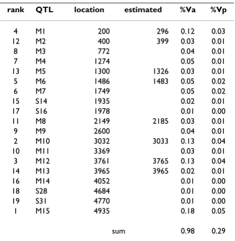
True positions of QTL were revealed after the workshop had taken place [7]. In Table 5 the estimated and true positions were compared. Eight of the 19 QTL (explaining 98% of the genetic variation) were found using our two-stage selective genotyping approach. About 54% of the genetic variance associated with these 19 QTL was covered by these eight QTL. Four additional QTL with smaller effects were also identified: S1 at 296 cM, S3/S4 at 513 cM, S21 at 3033 cM and S22 at 3048 cM. Additive QTL effects were not very well estimated, which might explain that Table 4: Genotypic effects of markers included in round 3 of the forward regression analysis (Standard errors of effects are given in italics).
genotype marker 11 12 21 22
296 0.000 0.050 0.134 0.307
0.000 0.118 0.122 0.121
399 0.000 -0.316 -0.393 -0.551
0.000 0.118 0.123 0.122
415 0.000 0.501 0.555 0.815
0.000 0.084 0.097 0.113
513 0.000 -0.331 0.102 -0.008
0.000 0.094 0.099 0.146
1326 0.000 0.223 0.164 0.449
0.000 0.095 0.097 0.099
1483 0.000 -0.214 -0.442 -0.570
0.000 0.107 0.104 0.107
2185 0.000 -0.198 -0.244 -0.472
0.000 0.078 0.092 0.115
3031 0.000 0.212 0.363 0.616
0.000 0.105 0.119 0.226
3033 0.000 0.400 0.574 0.980
0.000 0.098 0.118 0.133
3048 0.000 0.234 0.152 0.299
0.000 0.100 0.116 0.141
3765 0.000 0.490 0.556 1.004
0.000 0.091 0.094 0.102
3965 0.000 -0.164 -0.286 -0.630
0.000 0.083 0.093 0.135
Table 3: Significance of combined putative markers using forward regression, corrected for polygenic effects.
markers F-value df e var e var a h2 LogL diff AIC
Round 0 --- --- 4663 3.123 1.361 0.30 -5584
Round 1 1483 13.25 4651 3.104 1.002 0.24 -5466 130
3033 13.82
3048 9.32
3765 34.95
Round 2 1483 15.94 4639 3.096 0.895 0.22 -5441 167
3033 18.20
Round 3 1483 11.09 4627 3.085 0.827 0.21 -5430 190
Likelihood ratio profiles for chromosomes 1, 2, 3 and 4 with adjusted threshold
Figure 1
Likelihood ratio profiles for chromosomes 1, 2, 3 and 4 with adjusted threshold.
LRT for Tait Chr 1
LRT for Tait Chr4
some of the QTL with a smaller effect were not identified. The QTL at the beginning of chromosome 3 (SNP 2185), which was considered to be a false positive because it did not reach the significance level in the LDLA analysis, was in fact a QTL (M8) with a small effect.
The 2 stage approach reduced the number of genotypes from 28 million in the whole data set to 5.4 million in stage 1 plus 0.43 million in stage 2; a reduction of almost 80%. If SNP-genotyping allows for sufficient accurate esti-mation of allele frequency in pooled DNA, then only 540.000 genotypes have to be determined in the first stage, reducing the genotyping effort with another order of magnitude. The number of individuals to put into a pool depends on the accuracy of determining the allele frequency, which in turn depends on the method applied. With AFLP-markers the typical choice is to put 10 individ-uals in each pool [11].
Conclusion
The two-stage genotyping strategy with selective genotyp-ing detected regions with highly significant QTL useful for further fine-mapping. Large reduction of genotyping efforts saves costs which could be used for subsequent expression and functional analyses.
Competing interests
The authors declare that they have no competing interests.
Authors' contributions
HH and JB conceived the project. HH and SvdB analyzed the data. All took part in writing the paper.
Acknowledgements
This article has been published as part of BMC Proceedings Volume 3 Sup-plement 1, 2009: Proceedings of the 12th European workshop on QTL mapping and marker assisted selection. The full contents of the supplement are available online at http://www.biomedcentral.com/1753-6561/ 3?issue=S1.
References
1. Hillel J, Avner R, Baxter-Jones C, Dunnington EA, Cahaner A, Siegel PB: DNA fingerprints from blood mixes in chickens and tur-keys. Anim Biotechnol 1990, 2:201-204.
2. Michelmore RW, Paran I, Kesseli RV: Identification of markers linked to disease-resistance genes by bulked segregant anal-ysis: a rapid method to detect markers in specific genomic regions by using segregating populations. Proc Natl Acad Sci USA
1991, 88:9828-9832.
3. Darvasi A, Soller M: Selective DNA pooling for determination of linkage between a molecular marker and a quantitative trait locus. Genetics 1994, 138:1365-1373.
4. Korol A, Frenkel Z, Cohen L, Lipkin E, Soller M: Fractioned DNA pooling: a new cost-effective strategy for fine mapping of quantitative trait loci. Genetics 2007, 176:2611-2623.
5. Wang J, Koehler KJ, Dekkers JCM: Interval mapping of quantita-tive trait loci with selecquantita-tive DNA pooling data. Genet Sel Evol
2007, 39:685-709.
6. Dekkers JCM: Quantitative trait locus mapping based on selective DNA pooling. Anim Breed Genet 2000, 117:1-16. 7. [Http://www.computationalgenetics.se/QTLMAS08/QTLMAS/
DATA.html].
8. Janss LLG, Heuven HCM: LDLA, a package to compute IBD matrices for QTL fine mapping by variance components. Book of abstracts EAAP, Uppsala, Sweden; 2005:11.
9. Meuwissen THE, Goddard ME: Prediction of identity by descent probabilities from marker haplotypes. Genet Sel Evol 2001,
33:605-634.
Table 5: Simulated QTLs explaining more than 1% of the genetic variance and their true and estimated position and percentage of genetic (Va) and phenotypic (Vp) variance explained.
rank QTL location estimated %Va %Vp
4 M1 200 296 0.12 0.03
12 M2 400 399 0.03 0.01
8 M3 772 0.04 0.01
7 M4 1274 0.05 0.01
13 M5 1300 1326 0.03 0.01
5 M6 1486 1483 0.05 0.02
6 M7 1749 0.05 0.02
15 S14 1935 0.02 0.01
17 S16 1978 0.01 0.00
11 M8 2149 2185 0.03 0.01
9 M9 2600 0.04 0.01
2 M10 3032 3033 0.13 0.04
10 M11 3369 0.03 0.01
3 M12 3761 3765 0.13 0.04
14 M13 3965 3965 0.02 0.01
16 M14 4052 0.01 0.00
18 S28 4684 0.01 0.00
19 S31 4770 0.01 0.00
1 M15 4935 0.18 0.05
sum 0.98 0.29
Box-plot of estimated breeding values (EBV) of progeny of sire 389 by dam
Figure 2
Box-plot of estimated breeding values (EBV) of prog-eny of sire 389 by dam.
270 275 601 698 893 1186 1205
Publish with BioMed Central and every scientist can read your work free of charge "BioMed Central will be the most significant development for disseminating the results of biomedical researc h in our lifetime."
Sir Paul Nurse, Cancer Research UK
Your research papers will be:
available free of charge to the entire biomedical community
peer reviewed and published immediately upon acceptance
cited in PubMed and archived on PubMed Central
yours — you keep the copyright
Submit your manuscript here:
http://www.biomedcentral.com/info/publishing_adv.asp
BioMedcentral
10. Phiepo HP: A quick method for computing approximate thresholds for quantitative trait loci detection. Genetics 2001,
157:425-432.