Abstract
HEHR, BRIAN DOUGLAS. Development of the Thermal Neutron Scattering Cross
Sections of Graphitic Systems using Classical Molecular Dynamics Simulations. (Under the direction of Prof. Ayman I. Hawari.)
Proposed next-generation nuclear reactor concepts such as the High Temperature Gas Reactor (HTGR) and Very High Temperature Reactor (VHTR) incorporate graphite as a structural material and neutron moderator. The details of neutron slowing-down and thermalization in graphite impact the reactor energy spectrum, which, in turn, influences core design and fuel loading calculations. Of particular interest is the behavior of the graphite scattering cross section at thermal energies (below about 1 eV) where the interatomic binding environment of carbon atoms in the system determines the form of the differential cross section. In the absence of material-specific thermal cross sections, neutronics codes will, by default, utilize the free-gas approximation, which is commonly a drastic overestimation of the true cross section.
importance are detailed balance and atomic recoil, and a correction scheme has been developed herein to account for both. This correction takes the form of a transformation between the real and imaginary parts of the intermediate scattering function, established on the basis of a fluctuation-dissipation type relation. The transformed intermediate function is shown to produce consistent differential cross sections that are in agreement with ab-initio
based calculations. Furthermore, the transformation procedure is proven to reduce to the appropriate semiclassical limits at the extremes of small and large momentum transfers.
Correlations among the positions of distinct atomic pairs are also computed for the purpose of ascertaining the coherent inelastic cross section. These are validated against experimental measurements of the total scattering law and cross section of graphite. The Van Hove approach is markedly advantageous in this respect because the coherent inelastic component, which accounts for as much as 20-25% of the total graphite cross section, is inaccessible in
the LEAPR / NJOY formalism used to generate the standard ENDF/B-VII graphite libraries.
Total amorphization was also studied by melting and rapidly quenching the system at different densities.
For the purpose of studying the effect of damage on the cross section and frequency distribution, collision cascade concentrations were accumulated in an 8000-atom crystalline MD system. A transition from the crystalline frequency distribution towards the amorphous distribution was confirmed in the damaged region of the cell, associated with a dampening of the high-frequency in-plane optical modes of the vibrational spectrum, an enhancement of the out-of-plane modes, and a flattening of overall distribution. The total cross section was found to increase by as much at 48%, with the most significant change occurring in the 0.01-0.03 eV range.
Development of the Thermal Neutron Scattering Cross Sections of Graphitic Systems using Classical Molecular Dynamics Simulations
by
Brian Douglas Hehr
A dissertation submitted to the Graduate Faculty of North Carolina State University
in partial fulfillment of the requirements for the Degree of
Doctor of Philosophy
Nuclear Engineering
Raleigh, North Carolina
2010
APPROVED BY:
___________________ ___________________ Dr. Ayman I. Hawari, Dr. Mohamed A. Bourham Chair of Advisory Committee
Biography
Brian Douglas Hehr was born in Reading, Pennsylvania to parents Steven and Brenda Hehr. At the age of 3, Brian and his family moved to the vicinity of Charlotte, NC. Brian graduated from Sun Valley High School in 2000 and subsequently enrolled at North Carolina State University, where he graduated summa cum laude with dual B.S. degrees in physics and nuclear engineering. During his undergraduate studies, Brian participated in four summer internships – two at the Clariant Corporation headquarters in Charlotte and two at Los Alamos National Laboratory in New Mexico.
Acknowledgements
I would like to offer my heartfelt gratitude to Dr. Ayman Hawari for guiding my endeavors in this project and providing advice on both my Ph.D. work and future career. His ideas formed the foundation upon which the developments of this dissertation have matured. Dr. Hawari’s patience and motivation have been inspirational during my studies, and I aspire to emulate his dedication throughout my own career. I would also like to thank him for supporting my attendance at professional conferences, which has afforded me a valuable opportunity to communicate with others in my field.
The remaining members of my dissertation committee – Dr. Mohamed Bourham, Dr. Bernard Wehring, and Dr. Albert Young – deserve recognition as well for setting aside their valuable time to serve in this role.
Many thanks to Dr. Iyad Al-Qasir for always taking the time to talk with me, no matter how busy. I have learned much from his extensive knowledge of physics. I would also like to extend my appreciation to Dr. Victor Gillette for sharing his considerable programming experience as well as his expertise in a variety of topics.
Table of Contents
List of Tables ... vii
List of Figures ... viii
Chapter 1 Introduction ... 1
1.1 Overview ... 1
1.2 Forms of Graphite ... 4
1.2.1 Perfect Graphite ... 4
1.2.2 Reactor-Grade Graphite ... 6
1.3 Nuclear Cross Sections ... 8
1.4 Thermal Scattering Cross Section of Graphite ... 10
1.4.1 Overview of Thermal Scattering ... 10
1.4.2 Graphite Cross Section Calculations ... 12
1.5 Motivation and objective ... 15
Chapter 2 Molecular Dynamics ... 18
2.1 Overview ... 18
2.2 Potential Function ... 20
2.2.1 Introduction ... 20
2.2.2 REBO Potential ... 22
2.3 REBO corrections ... 23
2.3.1 Long Range Interactions ... 24
2.3.2 REBO pairwise adjustments ... 27
2.4 Correlation Functions ... 30
2.4.1 MD implementation ... 30
2.4.2 Cross-Correlation Theorem ... 33
Chapter 3 Thermal Neutron Scattering ... 35
3.1 Theory ... 35
3.1.1 Derivation from First Principles ... 35
3.1.2 Thermal Scattering Correlation Functions ... 41
3.1.3 Symmetry Relations ... 44
3.1.4 Moment Rules ... 46
3.1.5 Differential Cross Section from S(κ,ω) ... 47
3.2 Computational Methods ... 49
3.2.1 S(κ,ω) from ρ(ω) ... 51
3.2.1.1 Dynamical Matrix ... 53
3.4 Failure of Classical Formulation ... 65
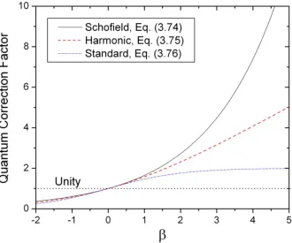
3.4.1 Semiclassical Corrections ... 69
3.4.2 Imaginary part of I(κ,t) ... 72
Chapter 4 Results for Perfect Graphite ... 78
4.1 ρ(ω) from MD ... 78
4.1.1 Dynamical matrix vs. velocity autocorrelation ... 78
4.1.2 Mismatch at Low Frequency ... 82
4.2 Heat Capacity ... 84
4.3 Dynamic Pair Correlation Function ... 86
4.4 Incoherent Thermal Scattering in Graphite ... 89
4.4.1 ρ(ω) from S(α,β) ... 92
4.4.2 Effect of Semiclassical Corrections ... 94
4.4.3 Classical / Quantum I(κ,t) Relation ... 101
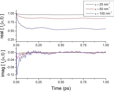
4.4.3.1 Intermediate Function ... 105
4.4.3.2 Scattering Law ... 108
4.4.3.3 Cross Section ... 110
4.4.4 Moment Analysis ... 111
4.4.5 Relaxing the Gaussian Approximation ... 113
4.4.6 Effect of Temperature ... 117
4.5 Coherent Scattering ... 121
Chapter 5 Results for Damaged Graphite ... 127
5.1 Introduction ... 127
5.2 Defect Formations ... 128
5.2.1 Simple Vacancy and Interstitial Defects ... 130
5.2.2 Heavily Damaged Systems ... 134
5.3 Stored Energy ... 138
5.4 Amorphous Carbon ... 140
5.5 Cross Section Impact ... 143
5.5.1 Cascade buildup at 300K ... 145
5.5.2 Cascade buildup at 800K ... 154
5.5.3 Impact of damage on ρ(ω) ... 156
Chapter 6 Conclusions and Future Work ... 160
References ... 166
Appendices ... 172
Appendix A ... 173
Appendix B ... 177
B.1 ρ(ω) from the Classical Scattering Law ... 177
B.2 ρ(ω) from the Quantum Harmonic Scattering Law ... 179
Appendix C ... 182
List of Tables
Table 1.1. Atomic number and moderating ratio of select moderators………..2 Table 2.1. Principal force constants of graphite………28 Table 2.2. Parameters for sigmoidal fit to C(T) ………...29 Table 5.1. Fractions of sp, sp2, and sp3 binding in the amorphous MD systems…………143
List of Figures
Fig. 1-1. Diagram of the Very High Temperature Reactor (VHTR) concept [1] . ... 1
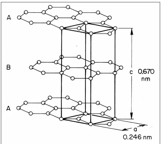
Fig. 1-2. Graphite structure and lattice parameters (at 0 K). The hexagonal unit cell of graphite is demarcated in bold lines... 4
Fig. 1-3. The hexagonal lattice. Elements of rotational symmetry are indicated by blue triangles. ... 5
Fig. 1-4. Schematic of a neutron scattering event ... 8
Fig. 1-5. The neutron scattering cross section at thermal energies. ... 10
Fig. 1-6. Comparison of the calculated thermal inelastic scattering cross section of pyrolytic graphite at 300 K, including 1-phonon coherent effects [14], versus measured data from Steyrel [16], Egelstaff [17], BNL [18], and Zhou [19],[20]. Triangles correspond to reactor-grade graphite while diamonds indicate pyrolytic graphite. ... 14
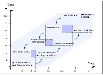
Fig. 2-1. Overview of multi-scale modeling ... 19
Fig. 2-2. Snapshots of an MD graphite supercell under the short-ranged REBO potential model. Distortion of the graphite planar structure occurs in the absence of long-range atomic interactions. ... 24
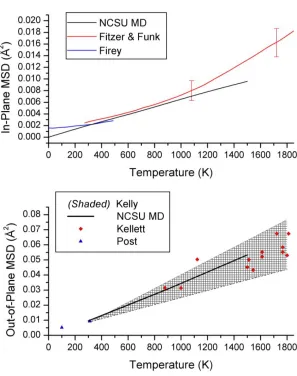
Fig. 2-3. In-plane (top panel) and out-of-plane (bottom panel) mean squared displacement in graphite. The in-plane MSD is compared against the x-ray diffraction measurements of Fitzer & Funk [30] and lattice dynamical calculations from Firey [31]. Out-of-plane MSD is shown alongside theoretical upper and lower bounds proposed by Kelly [32] as well as measurements performed by Kellet [33] and Post [34]. ... 27
Fig. 2-4. Impact of pairwise REBO adjustment factors on thermal expansion. The shaded region represents the total span of measured data reported by Billings [37], Steward [38] and Bailey [39]. ... 30
Fig. 3-1. Two approaches to computing S(κ,ω) from basic MD data ... 50
Fig. 3-2. Incoherent scattering law of Argon-40 at T = 85.5 K and ρ = 1.374 g/cm3 ... 63
Fig. 3-3. Coherent scattering law of Argon-36 at T = 120 K and ρ = 1.043 g/cm3. ... 64
Fig. 3-4. Zeroth moment of the liquid Argon-36 coherent scattering law at 120 K. ... 65
Fig. 3-5. The inelastic incoherent cross section of graphite versus its classical MD counterpart ... 66
Fig. 3-6. Differential energy spectrum of graphite at Einc = 1E-5 eV ... 67
Fig. 3-7. Differential energy spectrum of graphite at Einc = 5.1 eV ... 69
Fig. 3-8. Profiles of the Schofield, harmonic, and standard correction factors ... 71
Fig. 4-3. In-plane (top panel) and out-of-plane (bottom panel) partial frequency spectra of the MD graphite system. Out-of-plane motion is restricted only through the anisotropic cutoff function. ... 82 Fig. 4-4. Impact of the long-range force term on the graphite density of states ... 83 Fig. 4-5. Heat capacity of graphite, evaluated from the MD ρ(ω) ... 85 Fig. 4-6. Long-time limit of the classical dynamic pair correlation function of perfect
graphite ... 87 Fig. 4-7. Time dependence of the self part of G(r,t) at 300K. The displacement bin interval, Δr, is 0.01 Å. ... 89 Fig. 4-8. Classical moments of the MD-derived Scl(κ,ω) at 300 K... 91 Fig. 4-9. Phonon density of states as the low alpha limit of S(κ,ω) before collapsing the frequency domain (top panel) and after collapsing by a factor of 32 (bottom panel). ... 93 Fig. 4-10. Inelastic incoherent cross section at 300 K, with and without semiclassical
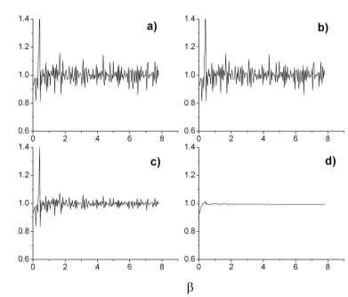
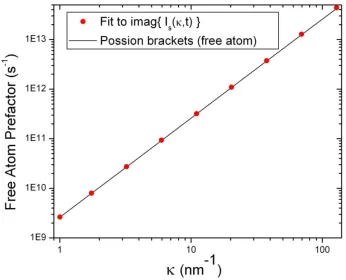
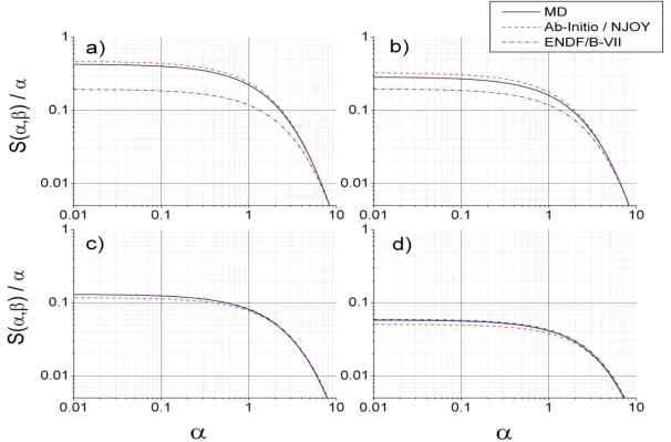
corrections to Scl(α,β). ... 95 Fig. 4-11. First moment of Ss(α,β), normalized to the theoretical value. ... 96 Fig. 4-12. Asymmetric scattering law as a function of positive beta, at select values of alpha. The harmonic semiclassical correction has been applied to Ss(α,β). ... 100 Fig. 4-13. Detailed balance ratio at a) α = 1E-4; b) α = 1E-3 ; c) α = 1 ; and d) α = 10. A ratio of unity indicates agreement with the detailed balance relation. ... 104 Fig. 4-14. Time dependence of the real and imaginary parts of Is(κ,t), Eq. (4.30), at 300 K. ... 105 Fig. 4-15. Time dependence of the real and imaginary parts of Is(κ,t), Eq. (4.30), at κ=500 nm-1 (in the free atom response regime of κ). ... 106 Fig. 4-16. Imaginary part of Is(κ,t), Eq. (4.30), in the short time limit ... 107 Fig. 4-17. Slope of the imaginary part of Is(κ,t), Eq. (4.30), in the short time limit vs. the predicted slope from the free atom Poisson bracket expression. ... 108 Fig. 4-18. Symmetric scattering law at 300 K and a) β = 0.2 ; b) β = 0.4 ; c) β = 0.8 ; and d) β = 1. ... 109 Fig. 4-19. Comparison of the total cross section generated under the proposed harmonic semiclassical and I(κ,t) transform schemes. ... 110 Fig. 4-20. Comparison of the differential cross sections generated under the proposed
harmonic semiclassical and I(κ,t) transform schemes at a) 1E-5 eV, b) 0.0253 eV, c) 0.184 eV and d) 5.1 eV. ... 111 Fig. 4-21. Computed moments of the MD scattering law. The first-order moment has been normalized by its theoretical value. ... 113 Fig. 4-22. Incoherent inelastic scattering cross section at 300 K, with and without the
Gaussian approximation... 115 Fig. 4-23. Incoherent inelastic cross section at 300 K, with and without the Gaussian
Fig. 4-26. Temperature dependence of the MD incoherent inelastic differential cross section
at a) 1E-5 eV, b) 0.0253 eV, c) 0.184 eV and d) 5.1 eV... 119
Fig. 4-27. Effect of temperature on the total inelastic incoherent cross section. ... 120
Fig. 4-28. Total inelastic cross section of graphite at 300 K. The experimental measurements of Steyrel [16] and Zhou [19] are shown as diamonds. ... 123
Fig. 4-29. Distinct differential cross section at a) 1E-5 eV, b) 1E-4 eV, c) 3E-3 eV and d) 0.025 eV. ... 124
Fig. 4-30. Total scattering law of graphite at 300 K, including coherent effects. ... 125
Fig. 4-31. Total scattering law of graphite at 533 K, including coherent effects. ... 126
Fig. 5-1. Accepted model of defect aggregations in graphite [74]. ... 129
Fig. 5-2. Steady-state structure of graphite following a 1 keV cascade. Only those atoms significantly affected by the cascade are included; the supercell itself extends far beyond the displayed region. ... 131
Fig. 5-3. Close-up view of a Stone-Wales defect from MD (left) and from ab-intio [76] (right). ... 131
Fig. 5-4. Stone-Wales defect in the context of a damaged basal plane. The heptagonal rings are marked with an “SW”. ... 132
Fig. 5-5. Defects within the graphite layer, from [77]. ... 132
Fig. 5-6. Interplanar divacancy defect: from ab-initio simulation [78] (left) and from MD simulation (right). ... 133
Fig. 5-7. Top view of the MD interplanar divacancy defect. Atoms colored in cyan form the top layer while atoms colored in grey comprise the bottom layer. The divacancy defect is evident near the center of the image. Other imperfections are also present such as the pentagonal rings in the top-left corner. ... 134
Fig. 5-8. A 24x24x4 graphite system before (left panel) and after (right panel) a series of 25 1-keV cascades initiated at random locations within the cell. Only the most heavily damaged region is shown here. ... 135
Fig. 5-9. Side view of one segment of a damaged MD graphite system. Extensive crosslinking has occurred between the planes ... 136
Fig. 5-10. Top view of the damaged segment. A line of vacancies cuts diagonally across the cell, forming a boundary between two continuous regions of the basal plane. ... 136
Fig. 5-11. Cross-linking of two planes, with the accompanying formation of vacancy lines (from [79]). ... 137
Fig. 5-12. Buildup of stored energy in a 300K MD graphite supercell ... 140
Fig. 5-13. Phase diagram of amorphous carbon, from [88]. The abbreviation ta-C refers to tetrahedral amorphous carbon. ... 141
Fig. 5-14. Snapshot of an MD amorphous carbon system at T = 300 K and ρ = 1.7 g/cm3. 142 Fig. 5-15. MD amorphous ρ(ω) versus the measured distributions of sputtered and glassy carbon. ... 142
Fig. 5-17. Damage effect on the total and differential cross section following (3) 1.5 keV cascades initiated at 300K………..147 Fig. 5-18. Damage effect on the total and differential cross section following (7) 1.5 keV cascades initiated at 300K………...148 Fig. 5-19. Damage effect on the total and differential cross section following (13) 1.5 keV cascades initiated at 300K………..149 Fig. 5-20. Effect of cascade buildup on the self part of the thermal scattering law following a) 1 cascade; b) 3 cascades; c) 7 cascades; and d) 13 cascades ... 150 Fig. 5-21. Effect of damage on the self part of Gcl(r,t). The displacement bin width, Δr, is 0.01 Å. ... 151 Fig. 5-22. Damage effect on the total and differential cross section following (3) 1.5 keV cascades initiated at 800K………..155 Fig. 5-23. Effect of cascade buildup on the self part of the thermal scattering law following (3) successive cascades at 800K. ... 156 Fig. 5-24. Effect of cascade buildup on the frequency distribution of graphite ... 157 Fig. 5-25. Ab-initio based calculation of the ρ(β) impact of adding an interplanar
Chapter 1
Introduction
1.1 Overview
At present, the majority of commercial power reactors are water-moderated. The resurgence of graphite has been driven by certain advantageous physical properties that include excellent mechanical strength, low density, high melting temperature, large heat capacity, and a low neutron absorption cross section. The standard metric for rating the effectiveness of a moderator is the moderating ratio, given by the formula:
s M
a
(1.1)
where Σs is the scattering cross section, Σa is the absorption cross section, and ξ, the average lethargy gain, is defined as:
2
1 1
1 ln
2 1
A A
A A
(1.2) in which A is the atomic mass number of the moderator. Essentially, ξ is a measure of the average energy lost by the neutron in a collision with a moderator atom. The purpose of the moderator is to deliver low-energy neutrons to the fuel; therefore, the moderating ratio is directly proportional to the lethargy gain and scattering cross section, and inversely proportional to the absorption cross section, which represents a neutron removal mechanism. The moderating ratio of several common moderator materials is tabulated in Table 1.1.
Table 1.1. Atomic number and moderating ratio of select moderators [2]
Moderator A ξΣs / Σa
H2O 1 (H),16 (O) 71 D2O 2 (D),16 (O) 5670
C 12 192
Deuterium oxide (heavy water) far outshines other moderators in terms ofM , chiefly
because of its tiny absorption cross section. This advantage is offset by the hefty price of manufacturing heavy water, as well as the requirement of a high pressure environment to prevent vaporization. The pressure constraint is particularly detrimental in new reactor designs such as the VHTR which emphasize high temperature operation as a means of increasing thermodynamic efficiency. Graphite, the second most effective moderator in Table 1.1, retains its structural integrity even at temperatures approaching the melting point of 3650˚C [3] – well above the expected accident temperature in a VHTR, for instance.
1.2 Forms of Graphite
1.2.1 Perfect Graphite
The graphite structure is illustrated in Fig. 1-2. In its perfectly crystalline state, graphite exhibits a hexagonal, planar configuration with ABAB type stacking. A rhombohedral form also exists with ABC stacking yet identical in-plane properties. Whereas neighboring layers of atoms are weakly bound through Van der Waals forces, the characteristic honeycomb structure of each plane is held together by strong covalent bonds, resulting in a high degree of anisotropy in the system properties. Two distinct atomic sites exist in graphite: one is distinguished by the presence of atoms directly above and below in neighboring planes (at
c/2) and the other by honeycomb gaps above and below.
To define the system mathematically, a grid of lattice points is constructed wherein the displacement between any two points is given by:
r AaBbCc (1.3) in which A,B, and C are integers and a, b , and c are the primitive translation vectors. Defining α, β, and γ as the angles between vectors b- c, a - c, and a- brespectively, the hexagonal lattice corresponds to the conditionsa b c, 0
90
and 0
120
. An example of a hexagonal lattice is shown in Fig. 1-3.
Fig. 1-3. The hexagonal lattice. Elements of rotational symmetry are indicated by blue triangles.
visualized as the product of infinite repetitions of the basis atoms. For graphite, there are four basis sites, which, specified as fractions of a unit cell, are:
C1: [0 , 0 , 1/4] C2: [0 , 0 , 3/4] C3: [1/3 , 2/3 , 1/4] C4: [2/3 , 1/3 , 3/4]
Since the basis positions and primitive vector angles are rigidly fixed in the hexagonal symmetry group associated with graphite, all that remains is to establish the lattice parameters, i.e. the unit cell scaling factors that generate the minimum-energy crystal structure at a given temperature. As depicted in Fig. 1-2, these are a = 2.46 Å (in-plane) and
c = 6.7 Å (out-of-plane) in 0 K graphite, resulting in a nearest-neighbor interatomic spacing of 1.42 Å. The phenomenon of thermal expansion (or contraction) arises from a temperature-dependent shift in the lattice parameters due to anharmonicity in the interatomic potential energy.
1.2.2 Reactor-Grade Graphite
to 2.25 g/cm3) [5]. Third, impurities that adversely affect reactor performance, such as boron, are largely removed in the production of reactor-grade graphite.
In addition to randomization in the orientation of crystallites, disorder is also observable in the interlayer spacing and stacking. Whereas perfect graphite exhibits a single, characteristic interlayer spacing in hexagonal form and a different, but still constant, spacing in rhombohedral form, the spacings in reactor-grade graphite are subject to variability. Deviations from the nominal spacing have been represented, in past work [6], using a Gaussian distribution. Moreover, the graphitic layers are turbostratic in reactor-grade such that adjacent layers may be translated or rotated randomly in relation to each other [7]. A consequence of this disorder is that the ABAB stacking sequence is broken, and, in fact, many of the characteristic powder diffraction peaks of graphite are broadened or lost entirely [8].
Bearing in mind the lower density of reactor-grade graphite as well as its coexistent phases, one would expect the properties of the reactor-grade and crystalline variants to diverge significantly. Indeed, the properties of reactor-grade graphite are much more isotropic due to the lack of a collective orientation (although some anisotropy still exists because of the
1.3 Nuclear Cross Sections
Consider a monoenergetic beam of neutrons incident on a thin slab of known composition. Assuming that attenuation is negligible within the slab, the neutron-nuclear reaction rate will be uniform and a cross section proportional to the probability of reaction can be defined as:
D
R N
(1.4)
where R is the reaction rate density, is the incident flux (# of neutrons per unit area per unit time) and ND is the atomic number density of the slab. Dimensionally, the nuclear cross section therefore represents an area, consistent with its original conceptualization as the effective “target area” presented to an incoming particle. While the cross section is a simple constant in this hypothetical example, a more constructive approach is to assign separate cross sections to different modes of interaction. The focus of this study is on scattering interactions in which the relevant neutron variables are the incident energy, scattered energy, and the scattering angle. A diagram of a neutron scattering event is shown in Fig. 1-4.
Fig. 1-4. Schematic of a neutron scattering event. The scattering element could be a single atom or a finite piece of a many-atom system. For the purpose of defining the cross section, it is assumed
The quantity of interest is the probability that a neutron of incident energy E will scatter into a solid angle dΩ about Ω with a final energy of dE’ about E’, where, in the notation of Fig. 1-4:
d sin d d (1.5) This probability is contained in the double differential scattering cross section, defined as:
' '
s N d
d dE d dE
(1.6) where Ns is the number of neutrons scattered per unit time into dΩ about Ω with a final
energy of dE’ about E’. From the definition, it follows that:
' '
d d
d
dE d dE
probability of scattering into dE’ about E’, regardless of Ω'
'
d d
dE
d d dE
probability of scattering into dΩ about Ω, regardless of E’' ' d d dE d dE
probability of scatteringIf the scattering event causes no change in the total kinetic energy, the scattering is labeled
1.4 Thermal Scattering Cross Section of Graphite
1.4.1 Overview of Thermal Scattering
When the incident energy of a neutron falls below approximately 1 eV, the atomic structure of a material exerts an appreciable influence on the scattering properties of the neutron. The reason is twofold: first, the neutron energy coincides with vibrational (phonon) energies of atoms in the crystal structure; second, the wavelength of the neutron is on the same order as the interatomic distances of the constituent atoms. Therefore, the neutron can be viewed as scattering from the collective structure rather than from any individual atom. The typical behavior of the cross section in the thermal scattering regime is illustrated in Fig. 1-5.
The underlying mechanisms of thermal scattering fall into two broad categories. Elastic
scattering can occur when the wavelength of the incident neutron satisfies Bragg’s diffraction law, given by:
n2 sind (1.7) where n is an integer, λ is the neutron wavelength, d is the spacing between atomic planes, and θ is the angle between the neutron and the scattering plane. Clearly, Bragg’s law yields a meaningful solution only in the case thatsin 1, thereby putting a lower bound on the neutron energy at which coherent elastic scattering is possible. For graphite, this minimum energy is about 2 meV and coincides with an abrupt spike in the cross section, apparent in Fig. 1-5 near the minimum point of the inelastic cross section curve. Coherent elastic scattering is not directly relevant to the thermalization process because only the direction of neutron propagation is affected. Therefore, this component of the cross section will be disregarded in the present work. Incoherent elastic scattering is important only for hydrogenous solids and will likewise be disregarded.
atoms. The scattering length of carbon-12 is overwhelmingly coherent and, consequentially, both mechanisms are important in graphite.
In the high energy limit – where the neutron wavelength becomes much smaller than the interatomic spacings – scattering interactions are well described by an elastic “billiard ball” model and the specific distribution of phonons is no longer important. Hence, the scattering cross section of any material approaches the free atom cross section in this limit, which demarcates the boundary between the thermal and epithermal regimes.
1.4.2 Graphite Cross Section Calculations
Presently, the standard approach to thermal cross section generation is to invoke approximations such that the double differential scattering cross section is reduced to an analytic function of the vibrational (phonon) density of states, ρ(ω). The LEAPR module of the NJOY code [9], for example, follows this methodology. If one chooses to work within the LEAPR framework, the main issue becomes the accurate determination of the density of states.
second, the fitting method is not predictive because the quantity of interest is forcibly conformed to measured data, rather than being constituted independently and then validated against measured data.
With improvements in computational power, it is now feasible to evaluate thermal cross sections through atomistic simulation. Recently, ρ(ω) has been calculated to high fidelity using the interatomic force constants obtained from ab-initio simulation. Because the details of interatomic interaction are treated quantum mechanically in ab-initio, no specific analytical model is needed to discern the force constants. Consequently, the empiricism of the earlier methods is avoided to a large extent.
Fig. 1-6. Comparison of the calculated thermal inelastic scattering cross section of graphite at 300 K, including 1-phonon coherent effects [14], versus measured data from Steyrel [16], Egelstaff [17], BNL [18], and Zhou [19],[20]. Triangles correspond to reactor-grade graphite while diamonds indicate pyrolytic graphite.
To summarize, the current state of knowledge regarding inelastic thermal neutron scattering in graphite is as follows:
Coherent and incoherent effects are both significant, with coherent inelastic scattering comprising as much as 20–25 % of the room-temperature cross section between 1E-5 and 5 eV.
The total inelastic scattering cross section of reactor-grade graphite is about 70% larger than that of pyrolytic graphite at 1E-3 eV. Differences are expected in the differential energy spectra as well.
1.5 Motivation and objective
presence of defects can result in a many-fold increase in the cost of evaluating the cross section, particularly when the simulated system is large. Size limitations are especially detrimental to irradiation studies since a large supercell is typically needed to observe properly the defect formation processes that arise during high-energy displacement cascades. In the case of time-independent ab-initio simulation, an initial guess of the defect structure would be required as input because the simulation technique does not allow for dynamical evolution of the system.
In contrast to the static ab-initio approach, classical molecular dynamics (MD) simulations run just as efficiently with imperfections as without, and are also suitable for dynamically modeling the defect accumulation processes responsible for lattice damage in a reactor environment. Classical MD, based on a well established interatomic potential function, therefore presents a more predictive (and computationally less intensive) approach for analyzing changes in the material structure and properties due to cascade buildup. Furthermore, Fourier transform techniques can be utilized to evaluate the thermal neutron scattering cross section directly from the atomic positions, without necessarily invoking the approximations embedded in codes such as LEAPR. This is possible through the use of statistical time correlation functions, which serve as a link between fundamental microscopic variables and measurable material properties.
impact of cascade-induced damage on the cross section. As will be demonstrated in Chapter 3, achieving these objectives also entails the development of quantum corrections to the classical Van Hove functions.
Chapter 2
Molecular Dynamics
2.1 Overview
Molecular dynamics (MD) is a simulation technique in which an interacting atomic system is evolved for a specified period of time under the laws of classical physics. Two preconditions are necessary in order to operate in the classical framework, namely that:
(1) Atoms can be treated as point masses, the motions of which are governed by Newtonian mechanics.
(2) Electrons are instantaneously in equilibrium with nuclei.
Item (1) is valid when the thermal de Broglie wavelength is much smaller than interatomic spacings in the material. The thermal wavelength is inversely related to both mass and temperature, and so an increase in either quantity will improve the appropriateness of this condition. Item (2) is an excellent approximation due to the vast mass difference between electrons and atomic nuclei.
the smallest scale that is currently practicable, quantum methods and approximations such as density function theory (DFT) can be used to investigate the electronic structure in addition to the atomic motions.
Fig. 2-1. Overview of multi-scale modeling
Some overlap exists between contiguous methods on the scale. For instance, the ab-initio
holistic perspective on multi-scale modeling, it is apparent that macroscopic phenomena could, in principle, be modeled from the most basic equations of quantum mechanics with few intermediate approximations. Limitations in computational power severely restrict the viability of this ideal at present. Much of the cost lies in evaluating the potential energy function (or Hamiltonian) of the system, along with its associated derivatives.
2.2 Potential Function
2.2.1 Introduction
Atomic interactions are modeled in MD using an empirically fitted potential energy function, the form of which is grounded in the specific nature of the system. In general, the potential function may be written as an expansion over 1,2,3, … N-body terms as:
1
2
,
3
, ,
... i i j
k j i k j i i i j
j i i
i V r r V r r r
r V
U (2.1)
where the potential is labeled an N-body potential when the expansion is carried out to VN.
Atomic interactions in graphite cannot be condensed into a simple 2-body potential. This is because the covalent interactions of graphite depend not only on the interatomic distances, but also on bond angles, torsional angles, and the coordination number. In other words, the potential energy is contingent upon the binding environment, and, for a given atom, the number of neighbor atoms affects the strength of each bond. It was this realization that led Abell [24] and later workers to develop the class of potentials known as bond order potentials. The theoretical basis for the bond order potentials lies in the derivation, from quantum mechanical equations, that:
k
Ak k Rk k qV p V Z
E (2.2)
2.2.2 REBO Potential
The 2nd generation reactive empirical bond order (REBO) potential [25] is presently one of the most sophisticated potential functions available for hydrocarbons. As with the Abell [24] and Tersoff [26] potentials, interatomic interactions in REBO are modeled as a sum of attractive and repulsive terms where the attractive part is modified by a bond order function. Mathematically:
i j i
ij A ij ij R ij
C r V r bV r
f
E (2.3)
where VR and VA are pairwise repulsive and attractive functions, bij is the bond order term,
ij
r is the scalar distance between atoms i and j, and fC
rij is a cutoff function that smoothly attenuates the potential energy to zero beyond the first neighbor shell. The repulsive and attractive components are given by:R 1 exp
ij
ij
Q
V A r
r
(2.4)
1,3
exp
A n n ij
n
V B r
(2.5)in which A, Q, , Bn, andn are empirical fitting constants. The exponential form of these functions is derivable from quantum formulae, but the
Q/rij
prefactor in VR was includedwith the specific intent of preventing atoms from approaching each other too closely during a high-energy collision (noting that the exponential terms saturate to a constant as rij 0).
bij
bij bji
ijRC bijDH2 1
(2.6)
where bij and b ji account for bond angles, ijRC is the bond conjugation term, and bijDH
represents the dihedral (torsional) contribution. The explicit forms of these functions are more intricate than the pairwise terms and are described in detail in the original paper [25]. The individual components of Eq. (2.6) share a common theme, however, in that each varies with the local atomic coordination number.
2.3 REBO corrections
Short-ranged empirical potentials are known to suffer from deficiencies that particularly impact anisotropic materials such as graphite. First and foremost is the absence of the long-ranged, interplanar Van der Waals interactions binding together graphite layers. Without an additional potential energy term to at least approximate the effects of these interactions, the graphite structure will be unstable.
Fig. 2-2. Snapshots of an MD graphite supercell under the short-ranged REBO potential model. Distortion of the graphite planar structure occurs in the absence of long-range atomic interactions.
The REBO potential, being a generalized hydrocarbon potential, was fitted to the static (zero temperature) properties of a range of hydrocarbon systems. Because the fitting procedure was performed at 0 K, there is no guarantee that temperature-dependent properties of the MD system will conform to experimental data, and adjustments may be needed to achieve agreement. Adjustments to the REBO potential, as applied to graphite, are expected to include the implementation of a Van der Waals potential as well as corrections to the empirical fitting parameters.
2.3.1 Long Range Interactions
12 6 4 LJ ij ij ij V r r (2.7)
in which ε and σ are empirical parameters that specify the depth and position of the potential energy well. Stuart, Tutein, and Harrison have recommended values of ε = 0.00284 eV and σ = 3.4 Å for graphite [27], where σ is approximately equal to the interlayer spacing. This parameterization is used in the present work.
At short distances (e.g. between 1st or 2nd neighbor shells), the Lennard-Jones potential interferes with the covalent terms of REBO by generating a strong repulsive force between atoms. Thus, the L-J potential is modified by a smooth, “reverse” cutoff function that tapers off the long-ranged potential between 3.40 Å and 3.00 Å, with no long range component present below 3.00 Å. These limits were chosen so as to be inclusive of nearest- neighbor interplanar interactions at (0,0,+c/2) or (0,0,-c/2).
As in prior versions of the modified REBO potential [28] , the standard cutoff function is replaced with an anisotropic function, defined by:
fc
rijz,T
fc rij fc
z,T' , ' (2.8) where:
2 2 cos 1 , ' d z K T z fc (2.9)structure, enables regulation of the c-axis mean-squared displacement independently of the in-plane displacements. For small displacements along the c-axis, fc'
z T, brings about a parabolic increase in energy with respect to the displacement.The parameter K was fitted to the out-of-plane mean squared displacement (MSD) for graphite, where the components of MSD are defined by:
2 0 1
2 2 2 o
T N t n n t T n
xy z
o r r
MSD MSD MSD r
N T T
(2.10)in which rnt refers to the instantaneous displacement of particle n at time t, N is the total
number of particles, To is the initial time step, T is the final time step, and (T-To) is the total number of time steps over which MSD is calculated.
Multiplying fc'
z T, through the pairwise attractive and repulsive terms gives a number with units of energy, and one would expect, on physical grounds, that:fc d T
VR
rij bijVA
rij
Ed ~ , 2 ' (2.11)
Fig. 2-3. In-plane (top panel) and out-of-plane (bottom panel) mean squared displacement in graphite. The in-plane MSD is compared against the x-ray diffraction measurements of Fitzer & Funk [30] and lattice dynamical calculations from Firey [31]. Out-of-plane MSD is shown alongside theoretical upper and lower bounds proposed by Kelly [32] as well as measurements performed by Kellet [33] and Post [34].
2.3.2 REBO pairwise adjustments
energy, bond distance, etc.) as determined for various hydrocarbon configurations. Notably, the fitting routine was limited to the static (0 K) properties of perfect lattices such that considerations of thermal motion were absent.
In the REBO formulation (and many others), a cutoff function limits interatomic interactions to the 1st neighbor shell. It is known, however, that 2nd neighbor atoms contribute significantly to the graphite potential. For example, Nicholson and Bacon [35] provide values for the principal force constants of the first two neighbor shells of graphite as listed in Table 2.1.
Table 2.1. Principal force constants of graphite in N/m, from Nicholson and Bacon
1st shell 2nd shell K11 323.36 -33.533
K22 279.95 91.44
K33 231.95 -38.533
At nonzero temperatures, it is expected that thermal vibrations and lattice expansion would perturb the longer-ranged interactions. These perturbations can be addressed by introducing a temperature-dependent adjustment factor that is fitted to the thermal expansion coefficient. Essentially, an adjustment factor is applied to the pairwise coefficients as:
A
T Aoexp
C
T T
(2.12) Bn
T Bn,oexp
nC
T T
(2.13) which accounts for deficiencies in the ability of the nearest-neighbor potential to accuratelymodel the true many-shell potential. Here, Ao and Bn,o are the standard REBO pairwise
coefficients and C(T) is a temperature-dependent adjustment factor, fitted to a sigmoidal function of the form:
d T T b c T C o o exp 1 )( (2.14)
in which co, b, d, and To are adjustable parameters. Using nonlinear least-squares regression (see [36] for more details), the parameter values shown in Table 2.2 were obtained, which correspondingly alter the thermal expansion behavior of the MD system to reflect the true expansion coefficient of graphite, as demonstrated in Fig. 2-4.
Table 2.2. Parameters for Sigmoidal Fit to C(T).
Fig. 2-4. Impact of pairwise REBO adjustment factors on thermal expansion. The shaded region represents the total span of measured data reported by Billings [37], Steward [38] and Bailey [39].
2.4 Correlation Functions
2.4.1 MD implementation
Correlation functions serve as the principal means by which material properties of relevance to engineering design can be related to the microscopic details of atomic motion. Aside from the thermal scattering correlation functions proposed by Van Hove, which constitute the foremost subject of development in the present work, there exists a class of Green-Kubo
relations are discussed further in Appendix A, in conjunction with their application to the specific property of the in-plane thermal conductivity of graphite.
The correlation of two stochastic random variables x and y is defined, in general terms, by a phase space integral of the form [40]:
Cxy
t t
E
t t
xy f
x y t t
dxdy
1 2
* 2
* 1 2
1
* , x y , ; , (2.15)
where x and y are construed as ensembles of possible outcomes, E{} is the expectation value,
x and y represent trial outcomes, and f
x,y;t1,t2
is the probability density of outcomes xand y occurring at timest1 and t2respectively. The implementation of this somewhat abstract formula in the context of an MD simulation is elucidated by considering the statistical mechanical interpretation of MD. From that perspective, the state of the MD system at time t
corresponds to a single point within the phase space of atomic positions
r and momenta
p . As the system evolves in time, transitions continually occur from one state to another, and the system history forms an increasingly long path in phase space that stretches from the initial state to the final state. While the system may pass through any accessible phase space point, certain states are more probable than others and so the calculation of averaged quantities must be weighted appropriately (as by the density function, f
x,y;t1,t2
, of Eq. (2.15)).
x
t y t
dt tC
t
t
xy
0 * *
1
lim
(2.16)
where is referred to as the delay time. Technically, the upper integration limit must approach infinity to ensure that the time evolution of the MD system encompasses all possible phase space configurations. Because real simulations cannot be infinite in duration, the system is taken to be adequately sampled after some finite time interval that depends on the initial state and intrinsic material properties. MD simulations also progress in discrete time steps and Eq. (2.16) therefore reduces to:
* * 1 1 Lxy k k
k
C x t y t
L
(2.17)in whichL
-- the number of steps available for averaging -- varies with the delay time. The relevant relationship is given by:
tot kL L
t
(2.18)
where Ltot is the total number of steps and must be an integer multiple of tk. A corollary of Eq. (2.18) is that the statistical uncertainty inCxy*
increases as a function of due to the linear drop in sample size. Hence, the time scale of the MD simulation may need to greatly exceed the characteristic time scale of the phenomenon under investigation, depending upon the desired degree of certainty.Cxy f
x
0 y t
(2.19)where f
x
0 y t
is defined as some function of the thermal average of the product x(0)y(t). Two distinct features of Eq. (2.19) are noteworthy:1. The time origin, t = 0, is arbitrary given that the system is in thermal equilibrium. Therefore, t actually refers to the delay time.
2. If the ergodic hypothesis holds, then the system is assumed to sample all accessible thermal states in its time evolution, and the thermal average, x
0 y t , is wholly identical to the time average of Eq. (2.17).2.4.2 Cross-Correlation Theorem
The calculation of correlation functions from Eq. (2.17) ordinarily entails on the order of N2
operations. When the signal size is large (more than, say, 104 – 105 points), this represents a significant computational burden, especially when multiple evaluations of the correlation function are required. Through implementation of the cross-correlation theorem, the number of operations can be reduced to NlogN with no loss in generality. As will be demonstrated later, cross section calculations can involve the computation of many thousands of correlation functions, and so the efficiency gain can be tremendous.
x y X
exp
2 i t d
Y*
' exp 2
i '
t
d' dt
(2.20)where x*y is the cross correlation of x and y, and X and Y are their Fourier conjugate variables. Combining the integrals on the RHS of Eq. (2.20),
x y X
Y* ' exp
2 i t
exp 2
i '
t
d d 'dt
X
Y* ' exp 2
i '
exp 2
it
'
dt d d '
X
Y* ' exp 2
i '
'
d d '
X
Y* exp 2
i
d
(2.21)which is simply the inverse Fourier transform of the product of the individual transforms of x
and y. If x = y, then Eq. (2.21) is equivalent to the Wiener-Khinchin theorem:
x x X
2exp 2
i
d
(2.22)which yields the autocorrelation of x.
Chapter 3
Thermal Neutron Scattering
3.1 Theory
3.1.1 Derivation from First Principles
In the thermal scattering regime, the neutron and scattering system both must be treated quantum mechanically. This is true because the wave properties of the neutron influence the scattering phenomenon (as is most obvious in coherent scattering), and also because the phonon energy exchange between the neutron and lattice is discretized in accordance with the energy levels of a network of quantum harmonic oscillators.
The state of the neutron is given by the Schrödinger equation [42]:
, 2
, , ,
2
r t
i r t V r t r t
t M
(3.1)
where V r t
, is the potential and
r t, is the wave function, the square of which is proportion to the probability of finding the particle at location r at time t. It can be shown that the wave function of a free particle (such as a traveling neutron), for which V r t
, = 0, is given by:
3/ 2
1, exp
2
free r t ik r i t
where k is the wave vector. The state of the scattering system,
r t, , is also governed by the Schrödinger equation; in the time-independent case this becomes a partial differential eigenvalue equation over 3(N+Ne) variables, where N and Ne and the number of nuclei and electrons respectively. Solving
r for a system of interacting atoms is the subject of theab-initio technique and density functional theory, in which the dimensionality of the problem is reduced considerably through a series of approximations. In general, however, the evaluation of
r t, is an intractable endeavor that, for the purposes of the present work, shall be deemed surmountable only in principle.Interaction between the neutron and scattering system alters the physical state of both entities, and the neutron scattering process can be conceptualized in terms of a differential cross section [43]:
, ', '
' '
1
k k k
d
W
d d
(3.3)that is proportional to the probability of transitioning from state k, to the set of
states k', ' , where k' is constrained to lie within the solid angle dΩ. If the transition
2 '
, ', ' '
2
' '
k k k
k
W k V k
(3.4)
k*' *V k drdR dR1 2...dRNwhere V is the nuclear potential acting on the neutron and ρk’ is the density of momentum states at k’ about dΩ. To proceed further, an explicit expression for the neutron-nucleus
potential is needed. The neutron, being an uncharged particle, interacts with the nucleus through the strong nuclear force, which is negligible beyond femtometer-scale separations. It is reasonable, therefore, to represent the potential as a delta function centered about the position of the nucleus as:
V r
a
r (3.5) where, for a single fixed nucleus, the constant a is given by the exact expression:
2
2 b
V r r
m
(3.6)
Combining the results of Eqs. (3.3)- (3.6), the differential cross section becomes:
2 ' ' ' exp j j j d kb i R
d k
(3.7)where κ = k’ – k is the change in the neutron wave vector due to scattering. Extension of this formula to the double differential cross section is straightforward – the energy of the scattering system plus neutron must be conserved during the scattering process; that is, E Ek E'Ek' (3.8) and the conservation of energy condition may be introduced as a delta function:
2 2 ' ' ' ' ' exp' j j j k k
d k
b i R E E E E
d dE k
(3.9)which is automatically normalized over energy. Now, at any given time, a realistic scattering system exists in one of many possible states (i.e. assumes one of an ensemble of states that are all consistent with the relevant conservation conditions). A well-known result of statistical mechanics [44] is that, at a constant temperature T, the probability of finding the system at energy Eλ is:
exp exp exp B B BE k T E k T
p
Z E k T
(3.10)where Z is the partition function. Converting the delta function of Eq. (3.9) to integral form through the relation:
' '
1 exp
'
exp
2
k k
i E E t
E E E E i t dt
(3.11)expiE t expiHtˆ
(3.12)
where ˆHis the Hamiltonian of the scattering system, the double differential cross section may be condensed into the following useful form:
2
' '
, ' '
exp 0 exp exp
' 2 j j j j j j
d k
b b i R i R t i t dt
d dE k
(3.13)with the atomic positions now defined as Heisenberg operators of the form:
j
exp ˆ jexp ˆiHt iHt
R t R
(3.14)
in which the details of the scattering system are confined to the position operator and scattering lengths. Significantly, the nuclear component of the differential cross section has been separated completely from the lattice dynamical component. This consequence of the Fermi pseudopotential approximation enables one to speak of thermal neutron scattering in terms of the dynamics of the scattering system.
Assuming that the system of interest contains a large number of nuclei, which is nearly always true in practice, the scattering length product may be substituted with a corresponding averaged value:
b bj j' b bj j'
and, if no correlations exist among the scattering lengths of different nuclei, then:
b bj j' bj bj' b 2 if 'j j (3.15)
b bj j' b2 if j' j (3.16) thereby causing Eq. (3.13) to split into two terms:
2 2 ' , ' 'exp 0 exp exp
' 2 j j j j
d k
b i R i R t i t dt
d dE k
(3.17)'
2 2
exp
0 exp
exp
2 j j j
k
b b i R i R t i t dt
k
Now, defining coh 4 b 2 and
2 24
inc b b
, the two terms on the RHS are seen
to correspond to the coherent and incoherent cross section respectively:
2
' , '
'
exp 0 exp exp
' 2 coh j j j j coh k d
i R i R t i t dt
d dE k
(3.18)
2
'
exp 0 exp exp
' 2 inc j j j inc k d
i R i R t i t dt
d dE k
(3.19)self correlations in addition to correlations among all of the distinct atomic pairs in the system.
3.1.2 Thermal Scattering Correlation Functions
Defining the intermediate scattering function as:
'
, ' 1
, exp j 0 exp j
j j
I t i R i R t
N
(3.20)and further defining the scattering law, or dynamic structure factor, as the time Fourier transform of the intermediate function:
,
1
, exp
2S I t i t dt
(3.21)Eqs. (3.18) and (3.19)can be expressed as:
2 ' , ' coh coh k d Sd dE k
(3.22)
2 ' , ' inc s inc k d Sd dE k
(3.23) with the total cross section equal to:
2
'
, ,
' coh inc s
d k
S S
d dE k
(3.24)
where the scattering law has been divided into a self and distinct part as:
![Fig. 1-6. Comparison of the calculated thermal inelastic scattering cross section of graphite at 300 K, including 1-phonon coherent effects [14], versus measured data from Steyrel [16], Egelstaff [17], BNL [18], and Zhou [19],[20]](https://thumb-us.123doks.com/thumbv2/123dok_us/1350701.1167948/28.612.122.515.88.405/comparison-calculated-inelastic-scattering-including-measured-steyrel-egelstaff.webp)