| INVESTIGATION
Signi
fi
cance Testing for Allelic Heterogeneity
Yangqing Deng and Wei Pan1 Division of Biostatistics, University of Minnesota, Minneapolis, Minnesota 55455
ABSTRACTIt is useful to detect allelic heterogeneity (AH),i.e., the presence of multiple causal SNPs in a locus, which, for example, may guide the development of new methods for fine mapping and determine how to interpret an appearing epistasis. In contrast to Mendelian traits, the existence and extent of AH for complex traits had been largely unknown until Hormozdiariet al.proposed a Bayesian method, called causal variants identification in associated regions (CAVIAR), and uncovered widespread AH in complex traits. However, there are several limitations with CAVIAR. First, it assumes a maximum number of causal SNPs in a locus, typically up to six, to save computing time; this assumption, as will be shown, may influence the outcome. Second, its computational time can be too demanding to be feasible since it examines all possible combinations of causal SNPs (under the assumed upper bound). Finally, it outputs a posterior probability of AH, which may be difficult to calibrate with a commonly used nominal significance level. Here, we introduce an intersection-union test (IUT) based on a joint/conditional regression model with all the SNPs in a locus to infer AH. We also propose two sequential IUT-based testing procedures to estimate the number of causal SNPs. Our proposed methods are applicable to not only individual-level genotypic and phenotypic data, but also genome-wide association study (GWAS) summary statistics. We provide numerical examples based on both simulated and real data, including large-scale schizophrenia (SCZ) and high-density lipoprotein (HDL) GWAS summary data sets, to demonstrate the effectiveness of the new methods. In particular, for both the SCZ and HDL data, our proposed IUT not only was faster, but also detected more AH loci than CAVIAR. Our proposed methods are expected to be useful in further uncovering the extent of AH in complex traits.
KEYWORDSCAVIAR; intersection-union test; statistical power; GWAS; conditional/joint modeling
T
HERE has been growing interest in detecting causal var-iants infine mapping for a disease or complex trait of interest, which can tell us about the biological mechanisms of the disease or trait. The most challenging part is to distinguish the true causal variants that biologically influence the trait and the variants that are only statistically associated due to link-age disequilibrium (LD) with the causal variants. A common approach is to use colocalization tests to infer whether a variant is causal for both the trait and a molecular intermediate trait like gene expression, through which the causal variant influences the trait. Many methods have been proposed for testing colo-colization, but most of them assume there is no more than one causal variant in each locus. When multiple causal variants exist, those methods may lose their effectiveness. As a result, it is important to know whether multiple causal variants are in alocus and, if so, how many they are. The presence of multiple causal variants in a locus is called allelic heterogeneity (AH). AH is known to be common for Mendelian traits, and it may also happen to common diseases and complex traits. In particular, its presence may influence the interpretation of some biological phenomena. For example, a previous study seemed to show that multiple epistatic effects affect gene expression (Hemaniet al.2014), which means that the effect of a variant on a trait is influenced by other variants else-where in the genome. However, according to Wood et al. (2014), most of those effects may be explained by a single third variant in that locus. This shows that the existence of AH or lack of it will critically determine whether there is an epistasis in a locus, and thus it is important to study AH.
One common approach to test AH is to use a so-called standard conditional analysis, in which one tests each SNP conditioning on the already detected significant SNPs (Yang et al.2012). This conditional analysis operates as a sequential forward variable/SNP selection procedure, which is known to be unstable and nonoptimal in general. Hormozdiariet al. (2017) proposed an alternative method called CAVIAR (causal variants identification in associated regions) that Copyright © 2018 by the Genetics Society of America
doi:https://doi.org/10.1534/genetics.118.301111
Manuscript received May 4, 2018; accepted for publication June 25, 2018; published Early Online June 29, 2018.
Supplemental material available at Figshare:https://doi.org/10.6084/m9.figshare. 6463292.
1Corresponding author: Division of Biostatistics, University of Minnesota, A460 Mayo
was proven to outperform the standard conditional analysis in most cases. However, since CAVIAR calculates the poste-rior probabilities for all possible subsets of causal SNPs, its computing time can be very long when the number of SNPs is huge. Accordingly, it imposes an assumption on the maxi-mum number of causal SNPs in a locus, say six, to save com-puting time. However, as will be shown, the assumed maximum number of causal SNPs will not only determine the computing time, but also influence thefinal result. Fi-nally, as a Bayesian method, CAVIAR gives the posterior prob-ability of AH; albeit useful, it may be difficult to calibrate a posterior probability with a commonly used statistical signif-icance level. For example, as will be shown, CAVIAR’s recom-mended significance cut-off of a posterior probability at$0.9 (to declare AH) may be too conservative when compared to a usual nominal family-wise type I error rate.
Technically, testing AH is similar to testing pleiotropy, which means that a SNP influences more than one trait. A direct way to test pleiotropy is to conduct the intersection-union test (IUT), which wasfirst mentioned by Schaidet al.(2016) and used by Deng and Pan (2017b). We propose a new hypothesis testing ap-proach to test for AH, based on the IUT with a joint/conditional model and the Wald tests. Note that our conditional model is based on the full set of the SNPs in a locus, differing from the standard conditional analysis of Yanget al.(2012) that is based on sequential forward variable/SNP selection, which is known to be unstable and nonoptimal with the cost of multiple testing/ selection. In contrast, our IUT is based on a full joint/conditional model on all SNPs, on which we test the null hypothesis of no AH directly, which is expected to be more powerful and stable than the sequential selection of SNPs. In particular, in the context of fine mapping, Benneret al.(2017) pointed out that the sequen-tial approach to conditional analysis is inferior to that based on the full joint/conditional model as adopted in FINEMAP (a soft-ware package for efficient variable selection using summary data from genome-wide association studies) (Benner et al. 2016). After determining the presence of AH, we also propose two se-quential testing procedures with IUT (Seq IUT) to infer the num-ber of causal SNPs. We will demonstrate the effectiveness of our new approaches with simulated and real data, including large-scale schizophrenia (SCZ) and high-density lipoprotein (HDL) genome-wide association study (GWAS) summary data sets.
Methods
Testing AH
Suppose we have the summary statistics of qSNPs on one trait, including the effect sizes, SE, and sample sizes. We can build a joint linear model of the traitvs.SNPs using the “jointsum” package provided by Deng and Pan (2017a). Denote the estimated coefficients and covariance matrix by
b
b¼ ðbb1:::bbqÞ9 and V. To testb H0: no more than one SNP
has a significant effect, we can use an idea similar to testing pleiotropy with the IUT, which was developed by Deng and Pan (2017b). We decomposeH0intoðqþ1Þparts:
H00: b1¼:::¼bq¼0;
H0j: b1¼:::bj21¼bjþ1:::¼bq¼0:ðj¼1; :::;qÞ:
For each individual test, we can use the Wald test statistic. The test statistic forH00isbb9Vb21bb, which followsx2ðqÞunder the null. The test statistic forH0jisbb2j9bV2j21bb2j, wherebb2jisbb
without thejth element, andVb2jis obtained by deleting the
jth row and column of V.b bb2j9bV2j21bb2j follows x2ðq21Þ
under the null. Then we can get theP-values for the
individ-ual tests, denoted by Pj ðj¼0; :::;qÞ. Since H0¼ [ q
j¼0H0j, we
can construct the IUT by taking P¼ max
j¼0;:::;qPj as the final
P-value. It is known that if each individual test is at level a, the overall test will also be at levela(Berger 1997).
Our above formulation follows that of Schaidet al.(2016) in the context of testing pleiotropy. As a reviewer points out,
since we haveH0 ¼ [q
j¼1H0j, we can construct the IUT by tak-ingP¼ max
j¼1;:::;qPjas itsfinalP-value; that is, we do not have to
useP0forH00. In theory, it is possible to have each H0j, but
notH00, rejected forj¼1; :::;q, we feel that conceptually it is better to includeH00to construct H0and thus the IUT, which might be slightly more conservative than otherwise.
Sequential testing
We propose a Seq IUT procedure to estimate the number of causal SNPs in the presence of AH, following the idea of Schaid et al.(2016). We can testHs*: onlyselements ofbare
non-zero using the same IUT approach. Hs* consists of HJ (J4ð1; :::;qÞ;jJj ¼s): the SNPs in J are causal, while the others are not. To test HJ, the Wald test statistic is
WJ¼bb2J9Vb2J21bb2J, wherebb2J,bV2J are obtained frombb, b
V after deleting the SNPs in J. Under the null,WJ follows x2ðq2sÞ. Then, we can calculate theP-value for each smaller test and compare the minimum witha. This IUT forHs* looks
at all the possible combinations of scausal SNPs and tests whether the remaining SNPs are all noncausal. If every com-bination is rejected, we can conclude that the number of causal SNPs is not equal tos. Since the number of possibilities may become too huge assgoes up, we also suggest setting a maximum number of causal SNPsk. The sequential testing procedure is:
1. TestH0* (no causal SNPs) at levelaby comparingbb9Vb21bb withx2ðqÞ. If we rejectH0
*, go to the next step; otherwise stop and conclude the number of causal SNPs is 0. 2. TestH1*,H2*, ...,Hk* one by one with IUT until thefirst
time that one of them is not rejected at level a. If Hm*
(m#k) is thefirst one that is not rejected, conclude the number of causal SNPs ism. IfH1*,H2*, ...,Hk* are all
rejected, conclude that the number of causal SNPs is big-ger thank.
sequential test is controlled at level aas well. Suppose the true number of causal SNPs ism. If we only testHm* at levela
with its IUT, the rejection probability isa. In the sequential procedure, we need to testH0*; H1*; :::; Hm* and reject all
of them to rejectHm*, so the probability of rejectingHm* is no
greater thana, the rejection probability of only testingHm*.
Since we need to consider all possibilities in each step of Seq IUT, it can be very slow when the number of SNPs is big. We propose a faster version of the procedure, called Seq IUT 2:
1. TestH0* andH1* in the same way as Seq IUT does. If both of them are rejected, test each SNP separately in the joint model andfind the most significant one, denoted byi1. 2. TestH2* with IUT; however, instead of considering all the
possible combinations of two causal SNPs, only consider the ones including SNPi1, which is assumed to be signif-icant already. There are onlyðq21Þcases left. IfH2* is rejected by IUT, test each possible combination of causal SNPs in the joint model andfind the most significant set, which isfi1;i2g.
3. Test H3*, assuming that i1 and i2 are significant and should always be included in the combinations of causal SNPs. This process is repeated until an insignificant result is obtained.
The difference between Seq IUT 2 and Seq IUT is that Seq IUT 2 keeps adding significant SNPs and thus is able to de-crease the number of combinations that we need to consider. In this way, not only is Seq IUT 2 faster, but it can also tell us which SNPs are significant. The two sequential procedures are conceptually similar to usual sequential procedures used in variable selection except that here we are testing AH, instead of testing the significance of individual parameters or being based on a model selection criterion like AIC (Akaike infor-mation criterion)/BIC (Bayesian inforinfor-mation criterion).
Data availability
The subset of the SCZ GWAS summary statistics (Schizophre-nia Working Group of the Psychiatric Genomics Consortium 2014) with the 103 loci after SNP pruning as used in this paper is available at https://doi.org/10.6084/m9.figshare.
6615461, while that of the HDL imputed GWAS summary
statistics (Pasaniucet al.2014) with the loci being used in this paper is available at https://doi.org/10.6084/m9.
figshare.6463292. The R packages“jointsum”and“AHIUT”
can be downloaded fromhttps://doi.org/10.6084/m9.figshare.
6615482andhttps://doi.org/10.6084/m9.figshare.6615470.
Results
Simulations
We conducted simulation studies that were similar to that of Hormozdiariet al.(2017). We looked at the 1000G (1000 Ge-nomes) CEU (Northern Europeans from Utah) population (1000 Genomes Project Consortiumet al.2015) with 503 sub-jects and chose some genes on chromosome 1 that had at least one SNP associated with some trait in the National Hu-man Genome Research Institute GWAS Catalog. For each gene, we deleted some SNPs to control all of the SNP pairwise correlations within 0.9. After excluding the loci with only one SNP, we ended up with 237 loci (genes) with eight SNPs on average in each locus. The range of the number of SNPs in a locus was 2–40.
Then, we simulated GWAS summary statistics with no epistasis interaction using the same approach as in Hormozdiari et al. (2017). Since we only needed the LD structure and effect sizes to simulate summary statistics in this scenario, we directly used the LD structureSestimated from the 1000G data and assumed that was the correlation structure for n¼1000 simulated subjects. In each locus, there were one or two causal SNPs, which were randomly decided. The normalized effect sizelof a causal SNP, defined aspffiffiffinb=swherebis the effect size andsis the SD of the error term, was chosen to be close to those in Hormozdiari et al.(2017). Denote the normalized effect size in a locus by L¼ ðl1:::lqÞ9. For a locus with one causal SNP, we assumed
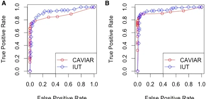
that the normalized effect size wasafor that SNP and 0 for the others. For a locus with two causal SNPs, the normalized effect size wasaandbfor those SNPs and 0 for the others. For instance, if thefirst and second SNPs in a locus are causal, the normalized effect size isL¼ ða;b;0; :::;0Þ9. If thefirst and Figure 1ROC curves for CAVIAR and IUT. (A)
last SNPs are causal, L¼ ða;0; :::;0;bÞ9, and so on. The summary statistics Z for that locus were simulated from MVNðSL;SÞ.
After obtaining the summary statistics and the LD structure for each locus, we carried out CAVIAR and IUT to get the posterior probabilities and P-values, respectively. Then, we compared the true positive rates (power) and false positive rates (type I error) using receiver operating characteristic (ROC) curves. Note that for the IUT, when we estimated the joint model, we tookZ as the marginal effect size and assumed that the SE was 1 and the sample size was 1000. We also directly used the LD structure estimated from the 1000G data. For CAVIAR, we set the maximum number of causal SNPs to six.
As shown in Figure 1, the performances of CAVIAR and IUT were close, though CAVIAR performed slightly better at extremely low false positive rates. Nevertheless, CAVIAR took much longer (at90 sec per data set) to run than IUT (at1 sec per data set). We can expect that if the number of SNPs is further increased, CAVIAR’s computation time will go up dra-matically because it compares Cðq;6Þ models per locus. Meanwhile, IUT will still be fast, since it only involves one model andðqþ1ÞWald tests per locus. We also repeated the process to generate multiple data sets and applied the meth-ods to all of them. The ROC curves did not change much.
In another simulation, we compared the IUT and CAVIAR in terms of detecting the number of causal SNPs. For each locus containing.12 SNPs, we assumed that there were one to three causal SNPs with the same effect size. We generated 10 data sets and applied the two approaches to calculate the true positive rates for different numbers of causal SNPs, de-fined as the proportion of the loci that were predicted cor-rectly. We chosek, the maximum number of causal SNPs, to be six for the methods.
The result is shown in Table 1. For Seq IUT, the number of causal SNPs was determined by when the sequential process stopped. For CAVIAR, the number of causal SNPs was the one
with the highest posterior probability; (*) determined the number of causal SNPs by requiring its posterior probability to be$0.8.
When the true number of causal SNPs was small, Seq IUT was much faster than CAVIAR, since it could come to an early stop instead of having to enumerate all possible combinations of causal SNPs. However, if the number of causal SNPs is larger, Seq IUT may lose its advantage, since it also needs to assess many possible combinations before it can stop. For instance, detecting 6 causal SNPs out of 40 SNPs using theforloop in R may take 8 min. Seq IUT 2 was faster than Seq IUT, and the speed advantage would be much larger as the number of SNPs went up. The result of Seq IUT 2 was also not much worse than that of Seq IUT.
SCZ data
To compare the performance of the methods on real data, we examined the reported 108 independent and significant loci in a SCZ GWAS (Schizophrenia Working Group of the Psychi-atric Genomics Consortium 2014), which gives the GWAS summary statistics based on 150,000 subjects. We chose the SNPs in the exact range of each genomic region that was reported by the Schizophrenia Working Group of the Psychiatric Genomics Consortium (2014), and then removed some SNPs in each region to ensure that none of the pairwise absolute correlations between any two SNPs was.0.9. Note that this procedure might be different from what was done by Hormozdiariet al. (2017), in which the data preprocessing procedure or definition of the significant loci was not pro-vided. We ended up with 103 loci containing multiple SNPs. We calculated the Z-scores using the reported odds ratio es-timates and the SE of log odds ratios, and then carried out the methods using the 1000G data as the reference panel (1000 Genomes Project Consortium et al.2015). For CAVIAR, we chose k based on q, the number of SNPs in a locus. The number of SNPs in a locus ranged from 3 to 407, with an average of 86. While the cut-off for the posterior probability Table 1 True positive rates for predicting the number of causal SNPs (k¼6)
CAVIAR (*) Seq IUT (Seq IUT 2)
No. causal SNPs 1 2 3 1 2 3
True positive rate 0.92 (0.008) 0.56 (0.016) 0.25 (0.057) 0.81 (0.81) 0.49 (0.39) 0.31 (0.30)
True negative rate 0.58 0.39 0.26 0.59 (0.65) 0.42 (0.43) 0.35 (0.41)
Computation time (seconds) 813 14 (13)
The computation time is for all loci. Normalized effect size = 4.89 or 0. CAVIAR, causal variants identification in associated regions; No., number of; Seq IUT, sequential intersection-union testing procedure.
Table 2 Numbers of significant loci with AH for SCZ
CAVIAR
IUT
a¼0:05=103 a¼531028
No. significant loci (overlap with CAVIAR) 28/32 60 (27/31) 49 (27/31)
Computation time (min) 9.9/2022 6.5
for AH was set to 0.8, as suggested by Hormozdiari et al. (2017), we tried two nominal significance levels for the IUT: one was based on a Bonferroni correction for testing the 103 loci, and the other was based on the usual genome-wide significance level (with a genome-wide scan).
As shown in Table 2, regardless of the significance level used, the IUT detected more significant loci than CAVIAIR, which was perhaps mostly due to the noncompatible signif-icance cutoffs between the two approaches. For the 18 AH loci detected by IUT (a¼531028) but missed by CAVIAR (with largerk’s), the mean posterior probabilities of having one and two causal SNPs were 0.364 (with range: 0.211– 0.608) and 0.369 (with range: 0.267–0.475), respectively; the mean posterior probability of AH was 0.635 (with range 0.387–0.789). For 10 out of the 18 loci, the number of causal SNPs being two yielded the highest posterior probability.
While CAVIAR became much slower askwent up, using a larger kled to more discoveries, demonstrating the impor-tance of specifying a largek at the expense of possibly too
long a computing time. The 32 significant AH loci identified by CAVIAR using larger kvalues covered the 28 identified with smaller k values. The one AH locus that IUT did not cover was the same as shown in Figure 4, which will be dis-cussed later. Note that our results from CAVIAR covered only some of the 25 loci reported in Hormozdiari et al.(2017), possibly due to different SNPs included in the loci. We also tried to define the loci by expanding from the lead SNPs and obtained similar results.
In Figure 2, for a locus with 38 SNPs, marginal analysis detected no significant SNPs among them, which means that the significant lead SNP was deleted in the pruning process. Meanwhile, the conditional analysis found multiple significant SNPs, three of which were highly significant. The IUT detected AH in this case (P-value = 2.7e214) and the Seq IUT method inferred the number of causal SNPs asfive. However, CAVIAR did not detect AH in this case (with a posterior probability of AH = 0.63 , 0.8). However, the posterior probabilities of having 0–2 causal SNPs were 0.0006, 0.37, and 0.47, respec-tively, with 0.47 being the highest among posterior probabilities Figure 2 Allelic heterogeneity in one locus associated with
schizophre-nia. (A) LocusZoom plot of 38 SNPs’P-values in marginal analysis. (B) LocusZoom plot of the same SNPs’P-values in conditional analysis. Hor-izontal line: significance cut-off 5e28. chr1, chromosome 1.
of having 0–6 causal SNPs, so CAVIAR would infer that the number of causal SNPs was two. This may indicate that, for CAVIAR, the results of testing AH andfinding the number of causal SNPs could be contradictory to each other.
As shown in Figure 3, in another locus with 31 SNPs, the marginal analysis found three significant SNPs, while the con-ditional analysis did not detect any. IUT concluded that there was no AH, and Seq IUT inferred the number of causal SNPs as zero, which agreed with the conditional analysis result. With the posterior probability of AH being 0.56, CAVIAR did not declare AH either. However, like the previous case, CAVIAR
suggested that the number of causal SNPs should be predicted as two, since its posterior probability was the highest (0.46).
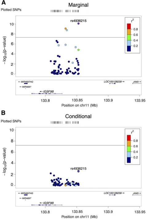
Figure 4 shows the only AH locus identified by CAVIAR but missed by IUT. The eigenvalues of the LD matrix for the SNPs in the locus ranged from 0.0018 to 10, suggesting that the LD matrix was not singular. CAVIAR inferred the number of causal SNPs as two, which were SNPs rs4936215 and rs695134; however, the conditional analysis said otherwise. The posterior probability of AH was 0.849, which was above the threshold of 0.8. The posterior probabilities of having 0–6 causal SNPs were 5.0e27, 0.15, 0.46, 0.28, 0.087, 0.017, and 0.0025, respectively. In contrast, the P-value of the IUT for testing AH was 0.019. Note that when we used 0.05 as the cut-off for IUT and Seq IUT, they detected AH and found two causal SNPs (rs12294011 and rs145205826). TheP-values of having one or less causal and two or less causal SNPs were 0.019 and 0.100, respectively. When we used the faster se-quential approach with a cut-off of 0.05, it detected three causal SNPs (rs12294011, rs145205826, and rs79071988); theP-values of having one or less, two or less, and three or less causal SNPs were 0.019, 0.027, and 0.061, respectively. The P-values for rs4936215, rs695134, and rs10894771 in the full conditional model were 0.003, 0.08, and 0.91, re-spectively, with the P-value of their joint test being 0.0063, while that of testing rs4936215 and rs695134 was 0.0069. Furthermore, we also tried forward sequential selection of significant SNPs one by one, which was the conditional method mentioned in Hormozdiariet al.(2017): in thefirst six steps, the six most significant SNPs (and theirP-value) were: rs4936215 (8.2e211), rs695134 (1.3e23), rs12294011 (8.3e23), rs4936214 (3.8e23), rs35261319 (0.014), and rs145205826 (0.0502). Hence, we conclude no strong evidence to support AH as reported by IUT.
HDL data
We also applied the methods to the summary statistics for HDL, imputed and provided by Pasaniuc et al.(2014). We focused on the 43 genes reported to contain SNPs associated with HDL in Teslovich et al. (2010) and used the 1000G reference again. The procedure was almost the same as that in the previous section for SCZ data. Each locus included the SNPs within 500 kb of the lead SNP. If any of the included significant SNPs (P-value,5e28) were 500 kbp upstream or downstream and correlated to the lead SNP (r2.0:1), they were expanded by 500 kbp in both directions as well. Before conducting the analyses, we deleted some SNPs to make sure Figure 4 One locus associated with schizophrenia. (A) LocusZoom plot of
68 SNPs’P-values in marginal analysis. (B) LocusZoom plot of the same SNPs’P-values in conditional analysis. Horizontal lines: significance cut-off 5e28. chr11, chromosome 11.
Table 3 Numbers of significant AH loci for HDL
CAVIAR
IUT
a¼0:05=43 a¼531028
No. significant loci (overlap with CAVIAR) 30/34 35 (28/32) 34 (28/32)
Computation time (hr) 0.3/42.4 9.4
that none of the correlations were.0.9 or, 20.9, while keeping the lead SNPs. When the LD matrix was nearly singular even after pruning, we took the generalized inverse of a matrix when needed, instead of the (ordinary) inverse, to avoid the numerical issue. However, when the number of SNPs was high, it was still possible to end up with a poor covariance matrix estimate for the regression coefficient es-timates with some negative diagonal elements. In this case, we applied a simple regularization method by adding a small constant (0.01) to the diagonal of the LD matrix and then dividing the whole matrix by 1.01 (to ensure its positivity).
In this case, IUT again detected no fewer significant AH loci than CAVIAR did, as shown in Table 3. The significant loci detected by CAVIAR covered 12 of the 13 significant loci reported by Hormozdiariet al.(2017). The difference was most likely due to different definitions of the loci. IUT be-came much slower as the number of SNPs bebe-came too high, because of its implementation in R (with its inefficiency of forloops and of inverting large matrices). For instance, with q¼1463 SNPs, the computation time of IUT was 4.3 hr, which could be improved by a implementation in a high-level language like C, as for CAVIAR. The two loci detected by CAVIAR but not IUT were the same for different choices ofk.
Discussion
Here, we have presented IUT for testing for AH, as well as Seq IUT and Seq IUT 2, two sequential testing procedures to infer the number of causal SNPs in the presence of AH. Our simulation results showed that the performance of IUT in terms of ROC was similar to that of CAVIAR, while the speed of IUT could be much faster, especially when the number of SNPs was not too small and not too big. After applying the methods to the large-scale SCZ and HDL GWAS summary data, we found more significant loci with AH using IUT than using CAVIAR with much less computational time. In addition, to save computing time in CAVIAR, one has to specify a relatively small number, k, of maximum causal SNPs for each locus; when applied to the SCZ and HLD data, we found that spec-ifying too large akcould take too much time, but at the same time, using a smallerkled to the detection of a smaller num-ber of AH loci by CAVIAR. We note that our statistical model for the joint distribution of the summary statistics in a locus is the essentially the same as that of CAVIAR. For predicting the number of causal SNPs, our proposed Seq IUT performed similarly to CAVIAR in the simulations, but it is expected to be faster, more so when the true number of causal SNPs is much smaller than the assumed maximum number of causal SNPs. The faster version, Seq IUT 2, further saves time, and its performance was no worse than that of Seq IUT in the simulations. The current speed advantage of our IUT-based methods over CAVIAR is expected to be more dramatic if we implement them in Rcpp (or a high-level language like C as for CAVIAR). Finally, we note that our statistical model for
the joint distribution of the summary statistics in a locus (as a multivariate normal distribution) is the essentially the same as that of CAVIAR. The main difference is that we separate the problem of testing AH from that of estimating the number of causal SNPs; the former is much faster than the latter, which requires some time-consuming exhaustive or sequen-tial searching.
Acknowledgments
This research was supported by National Institutes of Health grants R01 GM-113250, R01 GM-126002, R01 HL-105397, R01 HL-116720, and R21 AG-057038, by National Science Foundation grant DMS 1711226, and by the Minnesota Supercomputing Institute at the University of Minnesota.
Literature Cited
1000 Genomes Project ConsortiumAuton, A., L. D. Brooks, R. M. Durbin, E. P. Garrison et al., 2015 A global reference for hu-man genetic variation. Nature 526: 68–74. https://doi.org/ 10.1038/nature15393
Benner, C., C. C. Spencer, A. S. Havulinna, V. Salomaa, S. Ripatti
et al., 2016 Efficient variable selection using summary data from genome-wide association studies. Bioinformatics 32: 1493–1501.https://doi.org/10.1093/bioinformatics/btw018
Benner, C., A. S. Havulinna, M. R. Järvelin, V. Salomaa, S. Ripatti
et al., 2017 Prospects offine-mapping trait-associated genomic regions by using summary statistics from genome-wide associa-tion studies. Am. J. Hum. Genet. 101: 539–551. https://doi. org/10.1016/j.ajhg.2017.08.012
Berger, R. L., 1997 Likelihood ratio tests and intersection-union tests, pp. 225–237 inAdvances in Statistical Decision Theory and Applications, edited by S. Panchapakesan and N. Balakrishnan. Birkhäuser, Boston.
Deng, Y., and W. Pan, 2017a Conditional analysis of multiple quantitative traits based on marginal GWAS summary statistics. Genet. Epidemiol. 41: 427–436. https://doi.org/10.1002/gepi. 22046
Deng, Y., and W. Pan, 2017b Testing genetic pleiotropy with GWAS summary statistics for marginal and conditional analyses. Genetics 207: 1285–1299.https://doi.org/10.1534/genetics.117. 300347
Hemani, G., K. Shakhbazov, H.-J. Westra, T. Esko, A. K. Henders
et al., 2014 Detection and replication of epistasis influencing transcription in humans. Nature 508: 249–253.https://doi.org/ 10.1038/nature13005
Hormozdiari, F., A. Zhu, G. Kichaev, C. J.-T. Ju, A. V. Segrè
et al., 2017 Widespread allelic heterogeneity in complex traits. Am. J. Hum. Genet. 100: 789–802. https://doi.org/10.1016/ j.ajhg.2017.04.005
Pasaniuc, B., N. Zaitlen, H. Shi, G. Bhatia, A. Gusev et al., 2014 Fast and accurate imputation of summary statistics en-hances evidence of functional enrichment. Bioinformatics 30: 2906–2914.https://doi.org/10.1093/bioinformatics/btu416
Schaid, D. J., X. Tong, B. Larrabee, R. B. Kennedy, G. A. Poland
et al., 2016 Statistical methods for testing genetic pleiotropy. Genetics 204: 483–497.https://doi.org/10.1534/genetics.116. 189308
Teslovich, T. M., K. Musunuru, A. V. Smith, A. C. Edmondson, I. M. Stylianouet al., 2010 Biological, clinical and population rele-vance of 95 loci for blood lipids. Nature 466: 707–713.https:// doi.org/10.1038/nature09270
Wood, A. R., M. A. Tuke, M. A. Nalls, D. G. Hernandez, S. Bandinelli
et al., 2014 Another explanation for apparent epistasis. Nature 514: E3–E5.https://doi.org/10.1038/nature13691
Yang, J., T. Ferreira, A. P. Morris, S. E. Medland, P. A. F. Madden
et al., 2012 Conditional and joint multiple-SNP analysis of GWAS summary statistics identifies additional variants infl uenc-ing complex traits. Nat. Genet. 44: 369–375.https://doi.org/ 10.1038/ng.2213