DOI: 10.1534/genetics.107.071779
A Covariance Structure Model for the Admixture of Binary
Genetic Variation
Mark N. Grote
1Department of Anthropology, University of California, Davis California 95616 Manuscript received February 5, 2007
Accepted for publication May 25, 2007
ABSTRACT
I derive a covariance structure model for pairwise linkage disequilibrium (LD) between binary markers in a recently admixed population and use a generalized least-squares method to fit the model to two different data sets. Both linked and unlinked marker pairs are incorporated in the model. Under the model, a pairwise LD matrix is decomposed into two component matrices, one containing LD attributable to admixture, and another containing, in an aggregate form, LD specific to the populations forming the mixture. I use population genetics theory to show that the latter matrix has block-diagonal structure. For the data sets considered here, I show that the number of source populations can be determined by statistical inference on the canonical correlations of the sample LD matrix.
A
DMIXTURE, the mixing of genetically differenti-ated populations via migration and subsequent intermating, can create linkage disequilibrium (LD) between genes, even when the genes are not physically linked (see,e.g., Cavalli-Sforzaand Bodmer1971, p. 69; Prout1973). In this work, I show that admixture contributions to LD can be statistically quantified and distinguished from LD attributable to the shared ancestry of linked alleles. Ohta (1982) used Wright’s island model to decompose a squared coefficient of LD into within- and between-population terms, in analogy with Wright’s (1940) decomposition of the inbreeding coefficient. These decompositions assume that popu-lations connected by migration can be identified and sampled for genetic variation. The method I propose uses a pairwise LD matrix sampled from an admixed population of unknown composition; the number of source populations and the components of LD are in-ferred by use of a multivariate statistical model.The data: blocks of binary markers:It is convenient
to develop the model using gametes as the basic units of observation. The data are thennrandom binary vectors of the formx¼(x1,. . .xL)9, withxl2{0, 1};l¼1,. . .,L.
Each vector represents the single nucleotide polymor-phism (SNP) variation on one sampled gamete, under an arbitrary binary coding scheme, withxlindicating the
allele on gametexat thelth marker locus. The markers are assumed to be selectively neutral and variable in the sample.
Before statistical analysis begins, the markers inxare to be grouped intoblocksby the investigator, based on
physical criteria (e.g., the markers in a block share a localized region on a physical map), along with empir-ical evidence (e.g., the markers in a block are known by a previous linkage-mapping study to form a linkage group) independent of the sample under consider-ation. Each marker belongs to exactly one block; how-ever, a particular marker may be the only member of a block. Any two markers l, m within the same block are assumed to be linked, with recombination fraction clm>12. In contrast, markersl,jfromdifferentblocks are
assumed to be unlinked, with recombination fraction clj12.
In the development below, block structure derives from physical and linkage relationships between mark-ers, with blocks analogous to linkage groups; this is to be distinguished from empirical descriptions of ‘‘haplo-type block structure’’ (see, e.g., Gabriel et al. 2002; Phillipset al.2003). Recent work of the International HapMapConsortium(2005) and Myerset al.(2005) suggests that haplotype block structure results from variation in recombination rates over small physical dis-tances. The fine-scale rate estimates obtained by Myers et al. (2005) demonstrate new tools for constructing blocks of tightly linked markers. In the data examples to follow, I form two blocks of markers on the arms of the human X chromosome, using simple physical criteria.
To fix notation, I assume thatxcan be partitioned into Bblocks, labeled 1,. . .,Bin any convenient order (though the same partitioning and labeling scheme is used for all gametes). Forb¼1,. . .B, thebth block containsLb$1
marker loci, withPbLb ¼L. I order the vector elements
x1,. . ., xL so that the indices
P
a,bLa11;. . .;
P
a,bLa1Lb are assigned to the loci of thebth block.
However, markerswithina block need not be ordered in any particular way.
1Address for correspondence:Department of Anthropology, University of California, 1 Shields Ave., Davis, CA 95616. E-mail: [email protected]
For binary loci, linkage disequilibrium is covariance:
For binary loci, a familiar pairwise LD parameter (Lewontinand Kojima1960) is a covariance between locus-specific indicator variables. Letplbe the
popula-tion frequency of the ‘‘1’’ allele at locusl, letplmbe the
population frequency of gametes carrying the ‘‘1’’ allele at both locilandm, and letEbe the expectation operator for the distribution on (xl,xm)2{0, 1}3{0, 1}
parame-trized bypl,pm, andplm. The LD parameter for lociland
mis then
Dlm¼plmplpm¼EðxlxmÞ EðxlÞEðxmÞ ¼slm; l6¼m:
ð1Þ
For consistent definitions, I takeDllto be the variance of
the locus-specific indicator:
Dll ¼plpl2¼Eðx
2
lÞ ðEðxlÞÞ2 ¼s2l: ð2Þ Given a random sample of binary gametesx1,. . .,xn, withx¼n1Pn
1xi, I treat thel,mentry of the sample
covariance matrix
SL3L¼n1X
n
1
ðxixÞðxixÞ9 ð3Þ
as an estimate of Dlm. I use the denominator n in (3),
rather than the denominator n 1 typically used for unbiased estimation, for consistency with sample allele frequency calculations. The components of linkage dis-equilibrium under the admixture model are determined by the structure ofSand the sample allele frequencies. Other sample-based estimates of the population covari-ance matrix may provide suitable alternatives to S; the composite LD estimates described by Cockerham and Weir(1977; see also Weir1979) are particularly attrac-tive, as they do not require direct observation of gametes. A complete description of the associations among L binary markers requires the use of third- and higher-order moments, along with the second-order moments consid-ered here (see,e.g., Ekholm et al. 1995). Nonetheless, relevant structure in the data induced by admixture can be detected by an analysis limited to covariances.
In a recent article, Pattersonet al.(2006) also use a sample covariance matrix to make inferences about ad-mixture. Although the locus-specific variables defined by Pattersonet al.refer to diploid genotypes and take values in {0, 1, 2}, it is useful to establish a relationship between the matrix they analyze andS. In the notation above (up to differences in variable definitions, and omitting a normalization step), then3nmatrix of inter-individual covariances analyzed by Patterson et al. (2006) could be written as
L1ðx1x;. . .;xnxÞ9ðx1x;. . .;xnxÞ: ð4Þ Thus the implicit expectation is over loci rather than over individuals in the population, and covariances are
between multilocus genotypes rather than between locus-specific indicators. Wickens(1995) uses the terms vari-able spaceandsubject spaceto distinguish the multivariate spaces that give rise toS and (4), respectively. Gower (1966) and Jolliffe(2002, Sect. 5.2) compare and con-trast the two approaches, although a comparison in the context of admixture inference is beyond the scope of this work.
THE PULSE-DECAY MODEL OF ADMIXTURE AND A MATRIX DECOMPOSITION
The ‘‘pulse-decay’’ model (shown schematically in Figure 1) is a highly simplified admixture model that, somewhat unexpectedly, shares mathematical proper-ties with traditional covariance structure models. It is a variation of the ‘‘immediate admixture’’ model of Ewensand Spielman(1995), emphasizing different sta-tistical properties. I give a detailed derivation to show that the statistical model used later for data analysis is implied by the pulse-decay model.
Under the pulse-decay model, generation 1 of the admixed population consists of N diploid genotypes sampled at random with replacement fromK$2 source populations. The probability that a genotype is chosen from thekth source population isq(k).0;k¼1,. . .,K, with PK1 qðkÞ ¼1. The mixing proportions q(1),. . . q(K) are unknown. In practice,Kmay be an unknown parameter requiring estimation. A genotype contrib-uted by the kth source population consists of two gametes chosen at random with replacement from the 2N(k) gametes present at generation zero in the kth source population. At generation zero, the frequency of the ‘‘1’’ allele at locuslin source populationkispl(k),
k¼1,. . .,K, and the covariance between locilandmin source populationkisDlm(k). I call the vector of allele
frequenciesðp1ðkÞ;. . .;pLðkÞÞ9from source population kp(k), and I assume that the source population allele frequency vectorsp(1),. . .,p(K) are linearly indepen-dent. The latter assumption implies that the number of markersLis at least as large as the number of source populationsK. Linear independence ofp(1),. . .,p(K) also implies that no source population is an admixture of the other source populations. I describe the effect of weakening the assumption of linear independence briefly in a later section. Under the pulse-decay model, the source populations make no further contributions to the sampled population after generation 1. Mating is at random in the admixed population from generation 1 onward.
By straightforward calculation, the expected fre-quency of the ‘‘1’’ allele at locus l, at generation 1 in the admixed population, is p1;l ¼pl ¼
PK
D1;lm¼
PK
1
qðkÞðplðkÞ plÞðpmðkÞ pm Þ1PK 1
qðkÞDlmðkÞ;
m6¼l; PK
1
qðkÞðplðkÞ plÞ21PK 1
qðkÞDllðkÞ;
m¼l; 8
> > > > > > > < > > > > > > >
: ð5Þ
where Dll(k) is the locus-specific variance in the kth
source population.
The expected covariance in generation t 1 1, over realizations of the Wright–Fisher process in the ad-mixed population, is
EðDt11;lmÞ ¼ ðð1clmÞð1 ð2NÞ
1ÞÞtD
1;lm; m6¼l;
ð1 ð2NÞ1ÞtD
1;ll; m¼l;
ð6Þ
where clm¼ cml 2(0, 12 is the recombination fraction
between locilandm(see,e.g., Karlinand McGregor 1968, Equation 7). Weirand Cockerham (1974) pro-vide related expressions for ‘‘genotypic’’ disequilibria (see Weir1996, Chap. 3), which completely specify two-locus dynamics in diploid organisms. WhereasD1,lmof
Equation 5 is a population parameter, Dt11,lm of
Equation 6 is a random variable. In Equation 6, the valueclm¼0, corresponding to complete linkage of l
andm, is reserved for the varianceDll, where it gives the formula for the decay of heterozygosity in a finite popu-lation (seee.g., Crowand Kimura1970, Section 3.11). Examining Equation 6 with statistical modeling in mind, it is attractive to write therealized covariance in generationt11 as
Dt11;lm ¼rt;lmD1;lm; ð7Þ
where rt,lm¼rt,mlis an unknown parameter giving the
proportion of initial covariance (or variance) remaining after t transitions of the Wright–Fisher process. A sample from the admixed population in generationt1
1 produces an estimate ofDt11,lm, via thel,melement
of the sample covariance matrix. Although rt,lm is an
important structural component of the model, it will not be an object of estimation. To establish later math-ematical results, I assume that there existeandusuch that
0,e # rt;lm# u,‘; for alll;m: ð8Þ
This assumption places uniform upper and lower bounds on the extent to which covariances (or varian-ces) have decayed since the admixture ‘‘pulse,’’ for the loci included in the study. Covariances betweenunlinked loci (with clm ¼ 12) are expected to decay much more
quickly than covariances between linked loci: for un-linked loci, rt,lmis on the order of 2t. In light of this
observation, (8) significantly limits the number of generations that could have occurred since the admix-ture pulse. Assumption (8) also rules out changes in the signs of covariances, up to and including generationt1
1. The pulse-decay model is thus revealed to be pri-marily suited for recent admixture. Accordingly, any ad-ditional changes in allele frequencies and covariances due to mutation are assumed to be small enough to ig-nore, within the time-scale of the model.
Under the pulse-decay model, the realized covariance matrix in the admixed population at generation t11 can be written as
SLt131L¼Rt1GG9 1Rt1D[A1C; ð9Þ Figure 1.—Schematic of the pulse-decay model of admixture, showing representative pop-ulation parameters. Diagonal arrows indicate the transfer of randomly chosen genotypes, contrib-uted to the admixed population in the propor-tions q(1),. . ., q(K). Vertical arrows indicate transitions of the Wright–Fisher process in the admixed population. 2N(k) is the number of ga-metes present in source populationkat genera-tion 0, pl(k) and pm(k) are the frequencies of
the ‘‘1’’ allele at locil and m, and Dlm(k) is the
whereRL3L
t is the symmetric matrix havingl,melement rt,lm,1is the Hadamard (elementwise) product,
GL3K ¼pffiffiffiffiffiffiffiffiffiqð1Þdð1Þ;. . .;pffiffiffiffiffiffiffiffiffiffiqðKÞdðKÞ;
dðkÞL31 ¼pðkÞ p; k¼1;. . .;K;
p¼PK
1 qðkÞpðkÞ, and D
L3L is the symmetric matrix
havingl,melementPK1 qðkÞDlmðkÞ. The columns ofG are weighted vectors of source-population allele fre-quency deviations. The number of generations elapsed since the admixture pulse is assumed to be unknown. I do not propose to explicitly model time-dependent properties, but rather to model the effect of recent ad-mixture on observed covariances. Hence, the depen-dence ontis dropped in the final expression of (9).
The properties of A and C: The theory of
pop-ulation genetics predicts that covariances between un-linked loci will be negligible in the source populations, if the source populations are not very small. Here, I address the consequences of this prediction for C, along with other properties ofAandC.
In terms of understanding and specifying the model, much is gained by making clear how model parameters are derived from stochastically varying quantities. To de-scribe the association between alleles at locilandmin the kth
source population, I imagine a 2 3 2 table, formed from the set of gamete counts
NxlxmðkÞ : xl;xm2 f0;1g;NxlxmðkÞ$0;
X
xl;xm
NxlxmðkÞ ¼2NðkÞ
:
ð10Þ
The counts are arranged in the table in some natural way,e.g., by assigning rows to the alleles at locusland columns to the alleles at locus m. The following dis-cussion parallels Weir (1996, pp. 112–114), with the important exception that here the entire kth source population at generation zero plays the role of the ‘‘sample’’ in Weir’s development. Under the Wright– Fisher model, the gamete counts in (10) are random variables, having a multinomial distribution with param-eters 2N(k) andpðkÞ ¼ ðp11ðkÞ;p10ðkÞ;p01ðkÞ;p00ðkÞÞ; I specify the probabilitiespxlxmðkÞin more detail below for
the case of unlinked loci. I view thel,m-locus gamete counts in thekth source population at generation zero as a particular realization of (10), and the allele fre-quenciespl(k), pm(k) appearing in Figure 1 and
Equa-tion 5 as marginal frequencies of the realized 2 3 2 table. The covariance between xl and xm in the kth
source population, written as a function of the random gamete counts, is
DlmðkÞ ¼N11ðkÞ=2NðkÞ ðN11ðkÞ1N10ðkÞÞ
3ðN11ðkÞ1N01ðkÞÞ=ð2NðkÞÞ2: ð11Þ
I view the parameterDlm(k), appearing in Figure 1 and on
the right-hand side of Equation 5, as a realization ofDlm(k).
For unlinked loci l, m and 2N(k) sufficiently large, gamete frequencies follow the ‘‘independent loci’’ model (Ethier1979); under this model, the probability distribution on 232 tables has the property of row-by-column independence. Let pl(k) (respectively,pm(k))
be the probability that a randomly chosen gamete of the kth source population carries the ‘‘1’’ allele at locus l (m). Under the independent loci model, the multino-mial probabilities pxlxmðkÞ are p11(k) ¼ pl(k)pm(k),
p10ðkÞ ¼plðkÞð1pmðkÞÞ, p01ðkÞ ¼ ð1plðkÞÞpmðkÞ, andp00ðkÞ ¼ ð1plðkÞÞð1pmðkÞÞ. It is worth noting that the Wright–Fisher process in the kth source population need not be stationary in order for unlinked l, m to follow the independent loci model (Ethier 1979). Further, for large source populations, even weakly linked loci (those withclm, 12, but clmnot very
small) can be treated as independent (Ethier1979). By straightforward calculation, under the indepen-dent loci model,E(Dlm(k))¼0, where the expectation is over multinomial samples forming the kth source population at generation zero. For 2N(k) sufficiently large, a calculation using the ‘‘delta method’’ gives
VarðDlmðkÞÞ ¼EðD2lmðkÞÞ plðkÞð1plðkÞÞ
3pmðkÞð1pmðkÞÞ=2NðkÞ ð12Þ
(see Weir1996, Equations 2.17, 3.10), again assuming the independent loci model. As a consequence of the above, whenl,mare unlinked and 2N(k) is sufficiently large, the parameter Dlm(k) in Equation 5 can be
approximated by a normal deviate having mean zero and variance Q(k)/2N(k), where 0 , Q(k) , 1. Pro-vided that all of the source populations are sufficiently large, the parametersDlm(1),. . .Dlm(K) for unlinkedl,
m may then be viewed as a set of small, independent fluctuations about zero. I assume that the weighted average of these fluctuations, PkqðkÞDlmðkÞ, can be equated to zero for unlinked l, m. The fact that unlinked locil,mare assigned to different blocks leads to the observation that
clm¼rt;lmX
k
qðkÞDlmðkÞ ¼0;forl;min different blocks:
Consequently,Cis of block-diagonal form:
CL3L ¼
C1 0
1
0 CB
0 @
1
A; ð13Þ
whereCbis of dimensionsLb3Lb;b¼1,. . .,B.
The sub-matricesCb, formed by locus pairsl,min the
sameblock, contain covariances attributable to the shared ancestry of linked loci. Calculations of Ohtaand Kimura (1969) suggest the approximation VarðDlmðkÞÞ Q˜ðkÞ=
ð114NðkÞclmÞ, for linked loci with recombination frac-tionclm, where 0,Q˜ðkÞ,1. This variance characterizes
linked. For clm>12, Var(Dlm(k)) is nonnegligible,
com-pared to the scale of a sample covarianceslm. In the
pulse-decay model, theDlm(k) for linkedl,mare averaged over
source populations in order to form the elements of C1,. . ., CB. In contrast to the elements of the
off-diagonal-blocks, I do not equate the elements of C1,. . .,CB, to zero; yet, some elements ofC1,. . .,CB
may indeed be close to zero, if the covariancesDlm(k) for
linked loci tend to be of opposite signs in different source populations, and if the weightsq(1),. . .,q(K) are nearly equal. A scenario in which one source population has a relatively large mixing proportionqleads to a straightfor-ward interpretation of the elements ofC1,. . .,CB: here,
the elementclmmainly reflects the covariance between l,min the dominant source population.
The matrix A contains components of covariance resulting only from differences in allele frequencies be-tween source populations. These components are inde-pendent of any notion of physical linkage between loci, and could be considered entirely artifacts of admixture. A and C are symmetric by definition, and the following proposition establishes that both have the other essential property of covariance matrices. A proof is given in theappendix.
Proposition1.AandCare nonnegative definite.
In the remaining sections, I writeM$0 to indicate that a symmetric matrixMis nonnegative definite, andM.
0 to indicate thatMis positive definite.
The multiple battery factor analysis model: The
matrix A containing admixture covariances has a factorization given by the following proposition; the covariance structure model is then an immediate consequence. A proof is given in theappendix.
Proposition 2. There exists a matrix LL3(K–1) of full column rank such thatA¼LL9.
Proposition 2 establishes that the rank ofLis one less than the number of linearly independent source pop-ulation vectors p(1),. . ., p(K). Linear dependencies amongp(1),. . .,p(K), which could arise if the source populations are related by recent descent from an ancestral population, or are themselves connected by migration, will reduce the rank ofLaccordingly.
The matrix equation
S¼LL9 1C; ð14Þ
withCblock-diagonal, is a covariance structure model associated with the ‘‘inter-battery’’ (for B ¼ 2 blocks,
Tucker 1958) and ‘‘multiple battery’’ (for B $ 3,
Browne1980, Browneand Tateneni 1997) factor anal-ysis models of psychometrics. The preceding develop-ment has shown that the covariance structure Equation 14 is implied by the pulse-decay model. In psychometrics,
(14) is the covariance structure implied by the linear latent variable model
x¼m1Lf1z; ð15Þ
wheremL31andLL3(K–1)are unknown parameter matri-ces, f2 RK1 is a vector of unobserved ‘‘inter-battery’’ factors withE(f)¼0and Var(f)¼I, andz2RL
is a vector of unobserved ‘‘battery-specific’’ factors, independent of
f, withE(z)¼0and Var(z)¼C(see Browne1980). In ordinary factor analysis,Cis a diagonal matrix contain-ing the ‘‘unique variances’’ of the elements ofx(Lawley and Maxwell1971). The present statistical problem is to estimateLandCgiven an observationSofS.
Psychometric studies of ‘‘difficulty factors’’ (see,e.g.,
McDonald and Ahlawat 1974) caution against the
naı¨ve application of models (14) and (15) to binary data. However, alternative models for binary observations, including latent class and response function models (see e.g., Lazarsfeldand Henry1968; Bartholomewand Knott1999; Sattenet al.2001), assume that all pairs of observed variables are conditionally independent given the latent variables, and thus do not allow for the within-block covariances encoded in C. The block-diagonal structure ofCis an essential aspect of both the genetic model and the statistical methods described here.
ESTIMATION OF MODEL PARAMETERS
I first describe the basic model-fitting problem for an arbitrary number of blocks B; then in subsequent sections I discuss the cases B¼2 andB$ 3, and give two data examples.
ForLwith a given column rankK– 1, the parameters of the model (14) are said to beidentifiedif the map from (L,C) toSis one-to-one,i.e.,, if
ðL˜;C˜Þ 6¼ ðLˆ;CˆÞ0L˜L˜9 1C˜ 6¼LˆLˆ9 1Cˆ
( Jo¨ reskog1981). In practical terms, the identifiability of a model (or lack thereof) determines whether or not unique estimates of model parameters can be found, given the sample. When parameters of (14) are not identified, the strategy I adopt below is to obtain esti-mates which satisfy a generalized least-squares criterion. In particular situations I will describe, the parametriza-tionS¼A1Cis partly or wholly identified.
We know from population genetics that sample allele frequencies impose constraints on observed LD values, so it is natural to ensure that the same constraints apply to model estimates. As the diagonal element s2
l is the
sample variance of a binary variable, clearly
0#s2l #1
4: ð16Þ
For distinct locil,m, letalm ¼maxfˆplˆpm;ð1ˆplÞ ð1ˆpmÞgandblm ¼minfð1ˆplÞˆpm; ˆplð1ˆpmÞg, where
ˆpl,ˆpmare the sample frequencies of the ‘‘1’’ allele at loci
alm#slm# blm ð17Þ
(Lewontin 1964) derive from the fact that two-locus gamete frequenciesˆplmare nonnegative. Thomsonand
Baur(1984) described an additional set of inequality constraints on the elements ofS, deriving from the fact that three-locus gamete frequencies ˆplmj are
nonnega-tive. For the triplet of distinct locil,m,j, the constraints can be written as
slm1slj1smj$ ˆplˆpmˆpj ð1ˆplÞð1ˆpmÞð1ˆpjÞ;
ð18Þ
slmslj smj$ ˆplˆpmð1ˆpjÞ ð1ˆplÞð1ˆpmÞˆpj;
ð19Þ
slmslj1smj#ˆplð1ˆpmÞˆpj1ð1ˆplÞˆpmð1ˆpjÞ; ð20Þ slm1sljsmj#ˆplð1ˆpmÞð1ˆpjÞ1ð1ˆplÞˆpmˆpj: ð21Þ
Robinsonet al.(1991) determined that no additional constraints on the elements of S are imposed by considering loci in groups of four or more; thus, a complete set of inequality constraints can be obtained by applying (16) to the diagonal elements ofS, (17) to the elements involving distinct locus pairs l, m, and (18)–(21) to the elements involving distinct locus tripletsl,m,j. I will say that model estimatesLˆ andCˆ satisfy the constraintsCif (16)–(21) hold, upon replac-ing sample quantitiesslmby their estimatesðLˆLˆ9Þlm1
ˆ
Clm, forl,m2{1,. . .L}.
I use generalized least-squares (GLS) methods for fitting the model (14) to data for two main reasons: these methods do not require explicit distributional assumptions, and the statistical properties of GLS estimates are known under fairly general conditions (see,e.g., Browne1974, 1984; Jo¨ reskog 1981). For a ‘‘weight’’ matrix VL3L .
0 yet to be chosen, GLS estimates ofLandCare obtained by minimizing the discrepancy function
fVðL;C;SÞ ¼traceððSLL9CÞVÞ2
¼ kV1=2ðSLL9CÞV1=2k2 ð22Þ
on the set
fðL;CÞ: rankðLÞ ¼K1;C$0;ðL;CÞ
satisfy the constraintsCg;
wherek kis the Euclidean norm. I also examine the unconstrained problem, in which (22) is minimized on {(L, C): rank(L) ¼K – 1, C $ 0}; for, a minimizer
ðLˆ;CˆÞof the unconstrained problem may, for a given data set, satisfy the constraints C. In such a situation,
ðLˆ;CˆÞis also the minimizer of the constrained prob-lem. WhenVis not a function ofLorC, straightforward matrix differentiation (see,e.g., Magnusand Neudecker 1988, section 9.9) gives the estimating equations
@fV
@L¼2VðLL9 1CSÞVL¼0 ð23Þ and
@fV
@C¼B diag½VðLL9 1CSÞV ¼0; ð24Þ where for ML3L
, Bdiag½M gives M the same block-diagonal structure as C. Equations 23 and 24 give necessary conditions for a local (or global) minimum of fV, at a differentiable point of the parameter space (Magnusand Neudecker1988, Sect. 7.4).
In the following sections, I use weight matricesV.0 having the same block-diagonal structure asC. There are two main reasons for this choice: first, block-diagonal V can be chosen to reflect unique features (levels of polymorphism, etc.) of particular blocks; second, block-diagonal Vleads to a simple estimating equation for C. For block-diagonal V, pre- and post-multiplication byV1, along with straightforward matrix algebra, establishes that the necessary condition (24) is equivalent to
C¼B diag½SLL9: ð25Þ
Consequently, model estimates within diagonal blocks equal their observed counterparts:
ˆ
slm ¼ ðLˆLˆ9Þlm1Cˆlm ¼ ðLˆLˆ9Þlm1slm ðLˆLˆ9Þlm ¼slm; forl;min the same block: ð26Þ
THE MODEL WITHB¼2 BLOCKS
ForB¼2, it is convenient to write the two blocks of a gamete vector asxLx31andyLy31, withL
x1Ly¼L. The
covariance structure model (14) is then
Sxx Sxy
Syx Syy
¼ LxLx9 1Cx LxLy9 LyLx9 LyLy9 1Cy
; ð27Þ
whereLx,Lyare respectively of dimensionsLx3(K– 1),
Ly 3 (K – 1). I assume without loss of generality that
Lx#Ly.
Unfortunately,LandCare essentially unidentified for the model withB¼2 blocks. GivenLˆx,Lˆy,Cˆx, and
ˆ
Cy, which solve (27), many new solutions can be
generated by the family of transformations
ˆ Lx
ˆ Ly
!
1
ˆ LxM
ˆ LyM91
!
;
where M is any conformable, invertible matrix. All of these solutions will satisfy (27) for a given S; thus we need to impose additional criteria to choose a ‘‘good’’ solution from the many. Although L and C are not identified, the off-diagonal blocksAxy¼Ayx9, under the
˜
Axy6¼Aˆxy0S˜ 6¼Sˆ:
This parametrization is less informative mathematically, but shows that matrix elements describing admixture LD between loci of different blocks are unique.
I advocate a solution of model (27) first described by Rao(1973, 1979), and here give a rationale for its use in the admixture decomposition. I assume in the following thatSxxandSyyare nonsingular and that
K1#d[rankðS1=2
xx SxySyy1=2Þ:
The latter is a technical assumption which ensures that each latent dimension of the admixture model is repre-sented in the sample. The singular value decomposition (SVD) ofS1=2
xx SxyS
1=2
yy is accordingly
Sxx1=2SxySyy1=2¼UDW9; ð28Þ whereULx3LxandWLy3Lyare orthogonal,DLx3Ly ¼ ðD˜;0Þ,
˜ DLx3Lx ¼
diagðr1;. . .;rd;0;. . .;0Þ; andr1$$rdare thed#Lxsingular values.
The Rao (1979) solution for the model withB ¼2 blocks is
Lx*¼Sxx1=2UðK1ÞD1
=2
ðK1Þ;
L*y ¼S1yy=2WðK1ÞD1ðK=21Þ;
Cx*¼SxxLx*Lx*9;
C*y ¼SyyL*yL*y9; ð29Þ
where D(K–1) ¼ diag(r1,. . .rK–1), and U(K–1), W(K–1) respectively contain the columns ofU,Wcorresponding to the ordered singular values inD(K–1). The singular valuesr1$$rdofSxx1=2SxyS
1=2
yy , all of which lie in½0, 1,
are the sample canonical correlations between the variablesxandy.
The Rao solution can be connected to the uncon-strained GLS problem by a particular choice of V in (22), and by use of the corresponding necessary condition@fV/@C ¼ 0. A proof of the proposition is given in theappendix.
Proposition3.For
V¼ S
1
xx 0
0 S1
yy
! ,
the Rao solution(29)gives a global minimum of fV(L,C;S) on the set{(L,C):rank(L)¼K – 1,C$0}.
Thus the Rao solution is the GLS solution for the un-constrained problem, given the choice ofVimmediately above. Browne(1979) shows that the Rao solution (29) gives maximum-likelihood estimates of (L, C) in the multivariate normal setting, under additional identifi-ability conditions. The connection given by Proposition 3 between the Rao solution and the minimization of the GLS discrepancy function is apparently new.
There is no guarantee that the Rao solution (29) will satisfy the constraints C imposed by a given data set. Numerical methods for minimization of the discrepancy function (22), which explicitly incorporate inequality con-straints, have been described by Lee(1980); these remain an option if the fit of the Rao solution is unsatisfactory.
Data from The SNP Consortium: This is the first of
two data examples using SNPs organized into two blocks on the human X chromosome. My aim is more to show a proof of principle rather than to demonstrate any elaborations of the analysis. Although the examples may seem rather narrow, I do not intend that the method be limited only to very similar situations. In both examples I use only X chromosomes typed in males, in order to avoid any complications introduced by either inferring phase or estimating pairwise LD by indirect methods. Both data sets are, in a broad sense, deliberately admixed, as they combine population samples meant to characterize human ethnic or geo-graphic diversity. However, I will not assume that ethnic or geographic labels necessarily correspond to source populations, even if evidence for admixture is found.
The first data set is a sample ofn¼110 independent X chromosomes, typed by Celera Genomics as part of The SNP Consortium (TSC) Linkage Map Project (Clark et al. 2003; Matiseet al. 2003). Then¼110 males are comprised of the following (presumably self-identified) groups: 13 Asian males from the Celera diversity panel of 30 unrelated Asians; 15 African-American males from the Celera diversity panel of 30 unrelated African Americans; and 82 Caucasian males from the Utah CEPH pedigrees typed in ‘‘phase 2’’ of the Linkage Map Project. I selected CEPH males who could provide independent X chro-mosomes: typically for a three-generation pedigree, I included the father’s and paternal grandfather’s X chro-mosomes, along with a single X chromosome chosen at random from the maternal grandfather and sons.
The 11 SNPs used in this example are a subset of 39 X-linked SNPs typed by Celera Genomics in the diversity panels and CEPH Utah pedigrees. Two broad require-ments guided the selection of these SNPs. First, the SNPs can be assigned to two blocks located on different arms of the X chromosome (see Figure 2 for the physical map). Second, the number of parameters estimated in fitting the model with 11 SNPs is moderate, compared to the sample sizen¼110. With 11 SNPs there are 113
10/2¼55 population covariances estimated by sample statistics, along with 11 allele frequencies. There are at most 5 canonical correlations to include in the model, determined by the size of the smaller block. Once the number of canonical correlations to retain has been decided (by statistical inference), the other compo-nents of the Rao solution are uniquely determined. Thus in the present case there are at most 5511115¼
71 quantities to be estimated in fitting the model.
Inference of the number of source populations: In
turns the problem of inferring the number of indepen-dent sources into that of inferring the number of nonzero canonical correlations of the population LD matrix. Although test-statistics for making this inference exist, their null distributions are known only when the data are multivariate normal, or more generally are from an elliptically-contoured family (Muirhead and Waternaux1980). I use a bootstrap approach in order to avoid making assumptions about the data distribu-tion. It will be convenient to define some basic sample quantities: for i ¼ 1,. . .n, let xi¼ ðx1i;. . .xLxiÞ9, yi ¼ ðy1i;. . .yLyiÞ9be thexandyblocks of theith gamete, and
let X˜n3Lx
¼ ðx1x;. . .;xnxÞ9 , Y˜
n3Ly
¼ ðy1y;. . .;
ynyÞ9be the centered data matrices. The five sample canonical correlations for the TSC data are 0.46, 0.35, 0.25, 0.16, and 0.08.
The initial inference to be made is whether or not there is any support for admixture. For the pulse-decay model, this is equivalent to testing the null hypothesis that there is only one source population, hence no contribution from the term LL9 in (14). Under this hypothesisSitself is block-diagonal. A likelihood-ratio test for the null hypothesis of blockwise independence (block-diagonal covariance structure), assuming multi-variate normal data, is well known (see,e.g., Anderson 1984, Chap. 9; Seber1984, Sect. 3.5). ForB¼2 blocks, the test-statistic is
T0¼ ðn ðLx1Ly13Þ=2Þ Xd
i¼1
logð1ri2Þ; ð30Þ
wherer1$$rdare the sample canonical correlations
(Anderson1984, Sect. 12.4.1). For multivariate normal
data, the sample value t0 is compared to the x2 dis-tribution onLxLydegrees of freedom.
The null hypothesis of blockwise independence suggests a natural permutation strategy that I use to obtain a null distribution forT0: if the sample consists of pairs (x1, y1) ,. . ., (xn, yn), then a permuted sample under blockwise independence is (x1, yp(1)),. . ., (xn,
yp(n)), where p is a uniform random permutation of {1,. . .,n}. I computed the test-statisticT0for each ofR¼ 9, 999 permuted samples, and obtained an approximate p-value of
p ð11#ftr*$t0gÞ=ðR11Þ ¼0:019
for the test of blockwise independence, wheret1*,. . .,tR*
are the values of T0 for the permuted samples (see Davisonand Hinkley1997, Sect. 4.3). There is then good evidence against simple block-diagonal structure in the TSC data.
The permutation test does not extend readily to sequential tests which add nonzero canonical correla-tions to the model one at a time. So I proceed by computing sequential confidence regions, for the first canonical correlation, then for the first and second canonical correlations jointly, etc., by nonparametric bootstrapping. I take inclusion of the value zero in a confidence region as evidence that the corresponding correlation is nonsignificant.
Construction of a confidence interval forr1is the first step. I use a bootstrap approach described by Davison and Hinkley (1997, section 2.7.2) which employs smooth transformations of sample statistics and corre-sponding variance estimates. An approximate pivotal quantity can be obtained from the first sample canon-ical correlationr1using Fisher’s (1921) transformation
tanh1ðr1Þ ¼ ð12Þlogðð11r1Þ=ð1r1ÞÞ; ð31Þ
along with a variance approximation calculated from em-pirical influence values. The variance approximation is
v¼ ðnð1r12ÞÞ2X
n
j¼1
lj2;
where lj is the empirical influence value for the jth
observation on r1 (see Davison and Hinkley 1997, Equation 2.38). Guand Fung(1998) show thatljcan be written as
lj¼ ðsj1tj1r1ðsj211tj21Þ=2Þ; ð32Þ
wheresj1andtj1are thejth elements ofsn31 1¼Xa˜ 1and
tn31
1 ¼Yb˜ 1, respectively, andaLx
31
1 ,b
Ly31
1 are the sample canonical vectors associated withr1. The basic quantity to be bootstrapped is thenz¼v1=2ðtanh1ð
r1Þ tanh1
ðr1ÞÞ. The functionboot.ci, available in thebootlibrary of
the statistical software R (R Development Core Team 2005, version 2.2.1), handles the confidence interval calculations readily. A 95% studentized confidence in-terval forr1for the TSC data, obtained fromR¼9, 999 ordinary nonparametric bootstraps, is (0.18, 0.47), con-firming the existence of a first canonical correlation clearly distinct from zero. As the sample canonical correlation isr1¼0.46,r1is apparently highly biased as a naı¨ve estimator of r1. This can be confirmed by performing basic bootstraps ofr1.
Bootstrapping the first two or more canonical corre-lations together requires additional care: the noninde-pendence of the canonical correlations (imposed by their rank ordering) calls for joint bootstrapping and the use of a covariance matrix reflecting the joint structure. For a joint bootstrap of the first two canonical correlations, each transformed according to Fisher’s function, the covariance matrix estimate based on empirical influence values is d9Vd, where V232¼ n2Pn
j¼1ljl9j,
lj¼
sj1tj1r1ðsj211tj21Þ=2
sj2tj2r2ðsj221tj22Þ=2
!
; ð33Þ
d232¼diagðð1r12Þ1;ð1r2 2 Þ
1Þ;
sn31
2 ¼Xa˜ 2,t2n31¼Yb˜ 2, andaLx
31
2 ,b
Ly31
2 are the sample canonical vectors associated withr2(see Hampel et al. 1986, Equation 4.2.2; Davisonand Hinkley1997, Sect. 5.8). The basic quantity to be bootstrapped is then the quadratic form
q¼ ðhðrÞ hðrÞÞ9ðd9VdÞ1ðhðrÞ hðrÞÞ; ð34Þ
where
hðrÞ ¼ tanh
1ðr1Þ
tanh1ðr2Þ
:
The quantileqðð*1aÞ ðR11ÞÞ is the key quantity recovered
from the bootstrap samples; from this, a 100(1 –a)% joint confidence region for (r1,r2) is obtained as
fðr1;r2Þ:ðhðrÞ hðrÞÞ9ðd9VdÞ1ðhðrÞhðrÞÞ#q
ðð*1aÞðR11ÞÞg
ð35Þ
(see Davisonand Hinkley1997, Sect. 5.8). I checked the stability of the required matrix inversion by a preliminary bootstrap of the singular values of d9Vd. In the present case,d9Vdwas invertible in allR¼9, 999 bootstrap samples.
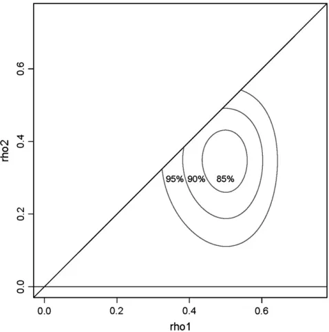
Figure 3 shows joint confidence regions for (r1,r2) based onR¼9, 999 bootstrap samples. The joint con-fidence regions clearly support the inference r1. 0, and give weaker, though measurable, support forr2.0. Before settling on a model with two canonical correla-tions, support forr3.0 needs to be investigated. I used
the natural extensions of (33)–(35) to three variables, to compute joint confidence regions for (r1,r2,r3) based onR¼9, 999 bootstrap samples. With three parameters the confidence regions are nested three-dimensional surfaces, similar to the Russian dolls known as ‘‘ma-treshki.’’ The nested surfaces are not easy to display graphically, so in Figure 4 I show theintersectionsof the surfaces with the two-dimensional (r1, r2) plane, in which r3 ¼ 0. Each of the three confidence regions intersects the plane, so I conclude that there is little support for a third canonical correlation. Thus the inference is that there aretwosignificant correlations in the TSC data, indicating the presence ofthree indepen-dent sources of variation.
Other methods for the TSC data:The computer
pro-gramStructure, available at http://pritch.bsd.uchicago.edu/ structure.html, implements Bayesian methods for fit-ting admixture models described in Pritchard et al. (2000) and Falushet al.(2003). Pritchardet al.(2000) describe a method for inferring the number of source populationsK, based on estimates of the probability of the sample given different values ofK. I usedStructure, along with rules of thumb described in the accompany-ing user’s manual, to infer the number of source populations for the TSC data, for comparison with the inference made above. For each of three models of ancestry implemented inStructure(the ‘‘no admixture’’, ‘‘admixture’’ and ‘‘linkage’’ models), I carried out five independent runs of theStructureprogram at each value
Figure 3.—Joint confidence regions for (r1, r2) for the TSC data, obtained by nonparametric bootstrapping. The 45° line and horizontal line through zero mark the region on which (r1,r2) are defined. Confidence regions are shown
ofK¼1,. . ., 5 (for a total of 75 runs). For each run, a ‘‘burn-in’’ of 100,000 iterations was followed by 1,000,000 Markov-chain Monte Carlo updates. Arguably, none of the ancestry models implemented inStructure are appropriate for the TSC SNPs, some of which are very tightly linked. Each ancestry model gave strongest support to the valueK¼1 for the TSC data. For models withK. 1, in all runs, the overall sample proportion assigned to a ‘‘cluster’’ was 1/Kfor each cluster. These re-sults are understood to indicate an absence of popula-tion structure.
The programs in Eigensoft (http://genepath.med. harvard.edu/
reich/EIGENSTRAT.htm) perform a prin-cipal components analysis described by Pattersonet al. (2006) for inference of admixture. Under this method, K– 1 is inferred as the number of statistically significant eigenvalues of an interindividual covariance matrix
½having a form similar to expression (4). As forStructure, I have reservations about using Eigensoft on the TSC sample, because the data architecture is of a form not intended by Patterson et al. (2006). In particular, Patterson et al. intend (but do not require) that the number of markers L be larger than the number of individualsn, and acknowledge that their method is not designed specifically to accomodate markers in linkage disequilibrium. I applied theEigensoftgenotype coding scheme to the TSC X chromosomes as follows: a male with the ‘‘reference’’ allele (chosen arbitrarily) at an X chromosome locus has the value 0 at the locus, whereas
a male with the ‘‘variant’’ allele has the value 2. I used the regression method described in Pattersonet al.(2006) to correct for LD, and varied the number of adjacent markers used for adjustment between 1, 2 and 3. In each caseEigensoftcalled all eigenvalues nonsignificant, thus the inference would be that only one population con-tributed to the TSC sample.
The admixture decomposition:The Rao solution can
be computed by straightforward matrix operations com-monly implemented in statistical or numerical pack-ages. I do the calculations in R (R DevelopmentCore Team2005, version 2.2.1), and describe a numerically stable method for computing the decomposition in the appendix.
The Rao decomposition for the TSC databased on two canonical correlations is shown graphically in Figure 5. The estimatesL*L*9 andC* satisfy the constraintsC
imposed by the sample allele frequencies. Covariances due to admixture, involving rs1541354 and rs1859004 (respectively, the third and fourth SNPs from the left in Figure 5) with several of the other SNPs, can be seen as vertical bands in the third and fourth columns of L*L*9. A comparison of the off-diagonal block of the residual matrix with the corresponding block of S
reveals a notable tendency for residual covariances to be corrected toward zero.
Data from the International HapMap Consortium:
In broad terms, the second example repeats the analy-sis of the TSC data, using a different sample of X chromosomes typed by the International HapMap
Consortium (2005), HapMap Public Release #21,
http://www.hapmap.org. Here I want to demonstrate that a different sample having similar structure yields similar results. The HapMap sample consists of 53 males of the Yoruban parent-offspring trios from Ibadan, Nigeria; 23 Japanese males from Tokyo; 22 Han Chinese males from Beijing; and 44 males of the Utah CEPH parent-offspring trios. Some of the Utah CEPH pedi-grees typed by Celera Genomics for TSC were also typed by HapMap; thus 20 of the Utah males I include in the HapMap sample were also in the TSC sample.
Although HapMap typed many more SNPs overall than TSC, the particular SNPs I used for the TSC sample were incompletely typed by HapMap. I elected to choose a new set of SNPs for the HapMap sample, located in the same X-chromosome regions represented by blocks 1 and 2 of the TSC sample. The HapMap browser locates the TSC SNPs of block 1 in the X-chromosome region 9.2 - 13.7Mb, and the SNPs of block 2 in 139.3 - 147.3Mb. I judged that a model with 15 SNPs would preserve a reasonable balance between sam-ple size (n¼142) and number of parameters. I chose 15 SNPs at random from those typed by HapMap, allocated to blocks 1 and 2 in rough proportion to the sizes of the two regions. Prior to choosing the 15 SNPs at random, I excluded SNPs from the two regions which had obvious genotyping errors or which failed to type in one or more
Figure4.—Intersections of the joint confidence regions for (r1,r2,r3) with the planer3¼0. The contours enclose portions
of the planer3¼0 contained in the three-dimensional
individuals. I discarded approximately three random SNP sets because the sample covariance matrices they produced were singular, or because the Rao decompo-sition based on 1, 2 or 3 canonical correlations would have failed to satisfy the constraints imposed by the sample allele frequencies. The latter biased the selec-tion toward a SNP set which yields a good fit of the model, but did not privilege any particular value ofK. Figure 6 shows the physical map of the 15 chosen SNPs. I used the same data analysis strategy for the HapMap sample as for the TSC sample, so I will summarize results briefly. The six sample canonical correlations for the HapMap data are 0.50, 0.41, 0.33, 0.23, 0.20 and 0.09. The permutation test of the statistic T0 produced an approximatep-value of 0.0007, indicating the presence of at least one significant canonical correlation. A 95% confidence interval for the first correlation is (0.25, 0.49), and joint confidence regions for the first two correlations are shown in Figure 7. The HapMap plot (not shown) analogous to Figure 4 has no contours in the (r1,r2) plane: thusr3¼0 is excluded from each of the 95, 90, and 85% confidence regions. I take this to imply support for a third correlation. Graphical display
of 4-dimensional regions is highly problematic, so I checked for the presence of a fourth significant corre-lation numerically. I bootstrapped the four-dimensional analog of (34) in order to estimate quantilesq*, then evaluated (34) at candidate points (r1,r2,r3,r4¼0), withr1,r2andr3varying in a region of high support. I found many such parameter combinations inside the joint confidence regions, and concluded that there is little evidence in the HapMap sample for a fourth correlation. Thus the inference is that there are three significant correlations in the HapMap data, indicating the presence offourindependent sources of variation. The Rao decomposition for the HapMap data, based on three canonical correlations, is shown graphically in Figure 8. The decomposition satisfies the constraintsC.
Other methods for the HapMap data:I followed the
same strategy usingStructureto inferKfor the HapMap data as for the TSC data. In contrast to the TSC data, Structure finds evidence for multiple clusters in the HapMap data; in particular, the ‘‘linkage’’ model pro-duces evidence for four clusters. In five runs of the linkage model withK¼4,Structureconsistently assigned overall sample proportions near 0.27 to three clusters, and 0.2 to a fourth cluster. Posterior probabilities of clus-ter membership suggest that most individuals are of mixed ancestry, having roughly equal proportions of their alleles assigned to two or more clusters.
I followed the same strategy using Eigensoft for the HapMap data as for the TSC data.Eigensoftcalls one ei-genvalue significant when either 1 or 2 adjacent markers are used for LD adjustment, and calls no eigenvalues sig-nificant when 3 adjacent markers are used. ThusEigensoft suggests that at most two sub-populations have contrib-uted to the HapMap X chromosome data.
THE MODEL WITH B$3 BLOCKS
Under mild conditions, the model withB$3 is iden-tified up to post-multiplication of Lby an orthogonal matrix (i.e.,up to rotations ofL). However, explicit for-mulae for parameter estimates are not readily available.
Figure 5.—Graphical representation of the covariance structure model fitted to the TSC data. The shaded squares depict absolute values of matrix elements below the main di-agonal, for the sample covariance matrixS, the matrix of es-timated admixture covariances L*L*9 (for the model with two canonical correlations), and the residual matrix S – L*L*9. The key, top right, gives the shading scheme applied to absolute values of matrix elements. The off-diagonal block containing covariances between SNPs of different blocks is marked by thick lines. The estimateC* is obtained by setting the elements of the off-diagonal block of the residual matrix equal to zero.
To fix notation, the block-partitioned parameter ma-trices areC, of the form (13), and
LL3ðK1Þ¼ L1
.. .
LB 0 B @
1 C A;
whereLbisLb3(K– 1);b¼1 ,. . .,B. ForB$3, Browne
(1980, Proposition 2) shows that a sufficient condition for identification ofC, and ofLup to rotations, is that at least three of the sub-matrices Lb of L be of full
column rank.
An assumption of the pulse-decay model, built on the notion thatL?K, is that the source-population vectors
p(1), . . . p(K) are linearly independent. If Lb, the
number of markers in thebthblock, is sufficiently large, it is reasonable to assume that linear independence also holds for the block-specific sub-vectorspb(1) ,. . .,pb(K). In fact, providedLb$K– 1, a block-specific version of
Proposition 2 (of this paper) is readily established, using suitably defined matricesGb, Abb, and a proof of the
same form. Browne’s Proposition consequently implies thatCis identified, andLis identified up to rotations, if Lb$ K– 1 for at least three blocks b2{1,. . . B}.
Fur-thermore, when at least three blocks meet this mini-mum size criterion, the matrixA¼LL9is unique: forA
¼LL9¼LQ(LQ)9whenQis orthogonal.
Obtaining an analog of Proposition 3 (of this article) forB$3 appears to be an open problem. Using
V¼
S111 0
1
0 SBB1
0 @
1 A;
C¼B diag½S–LL9and the reasoning of Proposition 3, GLS estimatesL* ,1 . . .,LB* for the unconstrained
prob-lem would be obtained by minimizing
f*ðL;SÞ ¼2X B
b¼1
X
i.b
kSbb1=2ðSbiLbL9ÞSi
1=2
ii k2: ð36Þ It is here that the strategy used for the model withB¼2 blocks breaks down, for although the Eckart–Young theorem (Gowerand Hand1996, Sect. A.4.4) can be used to minimize the individual summands of (36), it is not clear how to reconcile the different expressions for L* obtained asb ivaries.
At present, numerical estimation of (L,C) appears to be the only feasible option for the model withB$3. Lee (1980) gives algorithms for GLS estimation under parameter constraints, which are appropriate for the data under consideration. For inference ofK, anad hoc strategy involving sequential goodness-of-fit tests, simi-lar to a method used in ordinary factor analysis (see,e.g., Bartholomewand Knott1999, Sect. 3.8–3.9), may be pursued. For a candidate valueKand a GLS estimateL*, whereL* hasK– 1 columns, the fit of the model may be assessed by testing the residual matrix S – L*L*9for block-diagonal structure (see e.g., Anderson 1984, Chap. 9; Seber1984, Sect. 3.5); this assumes that such tests could be suitably adapted to multivariate binary
Figure 7.—Joint confidence regions for (r1, r2) for the HapMap data, analogous to Figure 3. The HapMap plot anal-ogous to Figure 4 has no contours in ther3¼0 plane.
observations. The smallest candidate valueKˆproviding the required block-diagonal residual matrix may be taken as an estimate ofK.
DISCUSSION
Here I have shown that a multilocus model of pairwise LD in an admixed population implies a particular covariance structure model (Equation 14), and that the model can be fitted feasibly to data. The simple pulse-decay framework will be implausible for many samples; nonetheless it may be useful to fit the statistical model, even when the form of admixture is clearly more complex, in order to discover or describe covariance structure. In this case, the ‘‘existence’’ result which con-nects the admixture model to (14) cannot be invoked: instead, it should be acknowledged that a convenient model of quasi-independent sources of covariance is being imposed on the data. The model (14), along with the statistical methods for fitting it, are of intrinsic interest and will likely have further applications in genomics. Regrettably, this description is too long to include work on a more general admixture model, in which source populations contribute to an admixed pop-ulation at each generation (e.g., the ‘‘gradual’’ admix-ture model of Ewensand Spielman1995). Preliminary calculations (not shown here) suggest strongly that a decomposition resembling Equation 9, involving a block-diagonal matrix and several non-block-diagonal matrices, will hold for the more general model. Ques-tions about the ranks of these matrices and about statis-tical inference in the general model remain for future work.
I can suggest two immediate, practical applications of this work. First, the model provides a well-supported statistical method for inferring the number of source populations contributing to an admixed population, for samples in which SNP markers can be organized into two blocks. In multiblock samples, the same method may still be applied by focusing attention on two well-chosen blocks. A complete extension of the method to multiblock samples is a desirable objective for future work. For the TSC and HapMap samples, I used canoni-cal correlations to infer the presence ofK¼3 andK¼4 independent sources of covariance, respectively. How-ever, the inferred sources need not correspond to the three (respectively four) groups defined in these samples by ethnic labels. Under the model, SNPs, not labeled individuals, come from independent sources.
A second application is the detection, through examination ofA*¼L*L*9, of SNPs worthy of scrutiny in an association mapping study, biogeography survey, or other context in which genetic mixtures are of interest. In both data examples considered here, exam-ination ofL*L*9revealed SNPs that had relatively large admixture LD in pairwise combinations with other markers. Such SNPs would be more likely to show ‘‘spurious’’
associations with phenotypic traits, in association-mapping studies not designed to detect admixture effects. The elements of C* are components of LD remaining after admixture artifacts have been removed; thus C* contains observed LD values adjusted for admixture effects. These quantities may provide suit-able surrogates for physical linkage in admixed popula-tions, similar to conventional LD measures in unstructured populations. We can imagine an association-mapping scenario in which a binary trait has been roughly mapped to a linkage group (say, represented by block 1), and it is desired to fine-map the trait in a potentially admixed population. We include the trait as a variable in block 1, and fit the covariance structure model to block 1 along with a second unlinked block, to detect associations between the trait and markers due to admixture alone. The elements of C* then give corrected components of LD between the trait and markers of block 1 and suggest which markers lay in close proximity to the trait locus.
I do not use the model to make inferences at the level of the individual, concerning, e.g., the proportion of alleles on a gamete inherited from a putative source population. The fine-grained information provided by the model consists of the matrix elements of the de-composition. Progress toward individual inference may be possible by noting that the canonical variable pairs (sk, tk); k¼ 1, . . . d, used here to calculate empirical influence values, are also used in classification and as-signment (see Krzanowskiand Marriott1995, Sect. 4.11). Formal inference at the individual level appar-ently requires estimation of individual factor scores f
in Equation 15. These factor scores are indeterminate from the view of multivariate analysis (see,e.g., Lawley and Maxwell 1971, Chap. 8; Mardia et al. 1979, Sect. 9.7): a single sample cannot be used to simulta-neously estimateL,C, and the individual factor scores
f1,. . .,fn.
of Romanazzi (1992) or Gu and Fung(1998). Geno-type-based influence values could then be used similarly to (32) and (33) in variance approximations. Du¨ mbgen (1998) gives an elegant method for constructing simul-taneous confidence intervals for canonical correlations. The numerical implementation of Du¨mbgen’s method requires only bootstrap realizations of the sample co-variance matrix, which could be formed by composite LD calculations on bootstrapped genotypes. A key quan-tity,b, used in Du¨ mbgen’s method is of order (L/n)1/2, and a small value ofbis desired to produce reasonably narrow intervals. After experimenting with Du¨mbgen’s method, I concluded that samples larger than the TSC or HapMap samples would be needed for successful implementation.
In fitting the model to data, I have stayed within relatively strict limits on the number of parameters esti-mated,vis a` visthe sample size, to avoid straining the statistical theory unduly. I view each sample covariance as an estimate of a population covariance parameter: thus the number of parameters of the model is a qua-dratic function ofL, the number of SNPs. Admittedly, using the sample size as an upper bound on the number of parameters of the model seems severe, at a time when thousands of SNPs can be typed simultaneously in an individual. However, allowing the sample size and num-ber of SNPs to be in the reverse relationship,n,L, calls upon multivariate theory still in early development.
Recently, Pattersonet al. (2006) have also taken a multivariate approach to the analysis of population structure. A thorough comparison of the method I have described with that of Patterson et al. will require significant work, although a few points of comparison can be discerned. Pattersonet al.note that blocks show-ing significant ‘‘standshow-ing’’ LD pose problems for their method, although they give an ad hoc strategy for handling this situation. The method I have described makes explicit use of such blocks, via the block-diagonal structure ofC. A key difference between the two ap-proaches is that Pattersonet al.decompose an n 3 n matrix of inter-individual covariances, whereas I de-compose anL3Lmatrix of covariances between SNPs. Under circumstances described by Gower(1966) and Jolliffe(2002, Sect. 5.2), there is adualityrelationship between subject-space and variable-space decomposi-tions. If a model in variable space dual to the model of Pattersonet al.can be described, it will be of interest to study the structure of the matrices analogous toLand C. Notably, Patterson et al. have developed their ap-proach with the relationshipn,Lspecifically in mind. Although they use multivariate theory forn,Lto the extent it is available, they necessarily rely on (well-argued) conjecture and numerical demonstration where theoret-ical results are lacking.
In my view, the relationship betweennandLis con-nected to basic notions of degrees of freedom. The need for theoretical and analytic tools suitable for genomic
data may prompt us to rethink how much can be inferred from a sample of fixed size. However, it seems prudent to admit from the start that the amount of information provided by a sample is limited and that the scope of inference should be limited accordingly.
I obtained the flat files TSCmap.p1.Celera.txt.gz and TSCmap.p2.Celera.txt.gz, from which the TSC data were extracted, at http://snp.cshl.org/. I obtained the flat files genotypes_chrX_CEU_r21_nr_fwd.txt.gz, gen-otypes_chrX_JPT1CHB_r21_nr_fwd.txt.gz, and geno-types_chrX_YRI_r21_nr_fwd.txt.gz, from which the HapMap build 35 data were extracted, at http://www. hapmap.org/. Python scripts used to perform data ex-traction and R scripts used to perform data analysis are available from the author.
Many thanks go to Chuck Langley; many of these ideas originated in discussions with him. Terry Speed and Matthew Stephens read early drafts of the manuscript, giving valuable comments and suggestions. Michael Browne, Lutz Du¨mbgen, Michael Perlman, and Yutaka Tanaka answered key questions about multivariate analysis. The comments of three anonymous reviewers on previous versions led to significant revisions. This work was supported by National Human Genome Research Institute (National Institutes of Health) grants 5R01HG002107-03 and 7R01MH60007.
LITERATURE CITED
Anderson, T. W., 1984 An Introduction to Multivariate Statistical
Anal-ysis,Ed. 2. Wiley & Sons, New York.
Bartholomew, D. J., and M. Knott, 1999 Latent Variable Models and
Factor Analysis.Arnold, London.
Browne, M. W., 1974 Generalized least-squares estimators in the
analysis of covariance structures. South African Stat. J.8:1–24. Browne, M. W., 1979 The maximum-likelihood solution in
inter-battery factor analysis. Br. J. Math. Statist. Psychol.32:75–86. Browne, M. W., 1980 Factor analysis of multiple batteries by
maxi-mum likelihood. Br. J. Math. Statist. Psychol.33:184–199. Browne, M. W., 1984 Asymptotically distribution-free methods for
the analysis of covariance structures. Br. J. Math. Statist. Psychol. 37:62–83.
Browne, M. W., and K. Tateneni, 1997 Noniterative estimation for
the multiple battery factor analysis model. Behaviormetrika24: 3–18.
Cavalli-Sforza, L. L., and W. F. Bodmer, 1971 The Genetics of
Hu-man Populations.W. H. Freeman, San Francisco.
Clark, A. G., R. Nielsen, J. Signorovitch, T. C. Matise, S. Glanowski
et al., 2003 Linkage disequilibrium and inference of ancestral re-combination in 538 single-nucleotide polymorphism clusters across the human genome. Am. J. Hum. Genet.73:285–300. Cockerham, C. C., and B. S. Weir, 1977 Digenic descent measures
for finite populations. Genet. Res.30:121–147.
Crow, J. F., and M. Kimura, 1970 An Introduction to Population
Genet-ics Theory.Burgess Publishing, Minneapolis.
Davison, A. C., and D. V. Hinkley, 1997 Bootstrap Methods and Their
Application.Cambridge University Press, Cambridge, UK. Du¨ mbgen, L., 1998 Perturbation inequalities and confidence sets
for functions of a scatter matrix. J. Multivariate Anal.65:19–35. Ekholm, A., P. W. F. Smithand J. W. McDonald, 1995 Marginal
re-gression analysis of a multivariate binary response. Biometrika 82:847–854.
Ethier, S. N., 1979 A limit theorem for two-locus diffusion models
in population genetics. J. Appl. Prob.16:402–408.
Ewens, W. J., and R. S. Spielman, 1995 The
transmission/disequi-librium test: history, subdivision, and admixture. Am. J. Hum. Genet.57:455–464.
Falush, D., M. Stephensand J. K. Pritchard, 2003 Inference of
Fisher, R. A., 1921 On the probable error of a coefficient of
corre-lation deduced from a small sample. Metron1:3–32.
Gabriel, S. B., S. F. Schaffner, H. Nguyen, J. M. Moore, J. Royet al.,
2002 The structure of haplotype blocks in the human genome. Science296:2225–2229.
Gower, J. C., 1966 Some distance properties of latent root and
vec-tor methods used in multivariate analysis. Biometrika53(3–4): 325–338.
Gower, J. C., and D. J. Hand, 1996 Biplots.Chapman & Hall, London.
Gu, H., and W. K. Fung, 1998 Assessing local influence in canonical
correlation analysis. Ann. Inst. Statist. Math.50(4): 755–772. Hampel, F. R., E. M. Ronchetti, P. J. Rousseeuwand W. A. Stahel,
1986 Robust Statistics: The Approach Based on Influence Functions. Wiley & Sons, New York.
Harville, D. A., 1997 Matrix Algebra From a Statistician’s Perspective.
Springer-Verlag, New York.
Horn, R. A., and C. R. Johnson, 1985 Matrix Analysis.Cambridge
University Press, Cambridge, UK.
InternationalHapMapConsortium, 2005 A haplotype map of
the human genome. Nature437(27): 1299–1320.
Jolliffe, I. T., 2002 Principal Component Analysis. Springer-Verlag,
New York.
Jo¨ reskog, K. G., 1981 Analysis of covariance structures. Scand. J.
Statist.8:65–92.
Karlin, S., and J. McGregor, 1968 Rates and probabilities of
fixa-tion for two locus random mating finite populafixa-tions without se-lection. Genetics58:141–159.
Krzanowski, W. J., and F. H. C. Marriott, 1995 Multivariate
Anal-ysis Part 2: Classification, Covariance Structures and Repeated Measure-ments.Arnold, London.
Lawley, D. N., and A. E. Maxwell, 1971 Factor Analysis as a
Statis-tical Method,Ed. 2. Butterworth, London.
Lazarsfeld, P. F., and N. W. Henry, 1968 Latent Structure Analysis.
Houghton Mifflin, Boston.
Lee, S. Y., 1980 Estimation of covariance structure models with
param-eters subject to functional restraints. Psychometrika45:309–324. Lewontin, R. C., 1964 The interaction of selection and linkage. I.
General considerations; heterotic models. Genetics49:49–67. Lewontin, R. C., and K. Kojima, 1960 The evolutionary dynamics
of complex polymorphisms. Evolution14:458–472.
Magnus, J. R., and H. Neudecker, 1988 Matrix Differential Calculus
With Applications in Statistics and Econometrics.Wiley & Sons, New York.
Mardia, K. V., J. T. Kentand J. M. Bibby, 1979 Multivariate Analysis.
Academic Press, London.
Matise, T. C., R. Sachidanandam, A. G. Clark, L. Kruglyak,
E. Wijsmanet al., 2003 A 3.9-centimorgan-resolution human
single-nucleotide polymorphism linkage map and screening set. Am. J. Hum. Genet.72:271–284.
McDonald, R. P., and K. S. Ahlawat, 1974 Difficulty factors in
bi-nary data. Br. J. Math. Statist. Psychol.27:82–99.
Muirhead, R. J., and C. M. Waternaux, 1980 Asymptotic
distribu-tions in canonical correlation analysis and other multivariate pro-cedures for nonnormal populations. Biometrika67:31–43. Myers, S., L. Bottolo, C. Freeman, G. McVeanand P. Donnelly,
2005 A fine-scale map of recombination rates and hotspots across the human genome. Science310:321–324.
Ohta, T., 1982 Linkage disequilibrium with the island model.
Genetics101:139–155.
Ohta, T., and M. Kimura, 1969 Linkage disequilibrium at steady
state determined by random genetic drift and recurrent muta-tion. Genetics63:229–238.
Patterson, N., A. L. Priceand D. Reich, 2006 Population structure
and eigenanalysis. PLoS Genetics2: 2074–2093.
Phillips, M. S., R. Lawrence, R. Sachidanandam, A. P. Morris, D. J.
Baldinget al., 2003 Chromosome-wide distribution of
haplo-type blocks and the role of recombination hot spots. Nat. Genet. 33:382–387.
Pritchard, J. K., M. Stephensand P. Donnelly, 2000 Inference of
population structure using multilocus genotype data. Genetics 155:945–959.
Prout, T., 1973 Appendix, pp. 494–496 in Mitton, J.B., and
R.K.Koehn, 1973, Population genetics of marine pelecypods. III. Epistasis between functionally related isoenzymes ofMytilus edulis.Genetics73:487–496.
R DevelopmentCoreTeam, 2005 R: A Language and Environment for
Statistical Computing. R Foundation for Statistical Computing, Vienna. http://www.r-project.org.
Rao, C. R., 1973 Linear Statistical Inference and Its Applications, Ed. 2.
Wiley & Sons, New York.
Rao, C. R., 1979 Separation theorems for singular values of matrices
and their applications in multivariate analysis. J. Multivar. Anal.9: 362–377.
Robinson, W. P., M. A. Asmussenand G. Thomson, 1991
Three-locus systems impose additional constraints on pairwise disequi-libria. Genetics129:925–930.
Romanazzi, M., 1992 Influence in canonical correlation analysis.
Psychometrika57:237–259.
Satten, G. A., W. D. Flandersand Q. Yang, 2001 Accounting for
unmeasured population structure in case-control studies of genetic association using a novel latent-class model. Am. J. Hum. Genet.68:466–477.
Seber, G. A. F., 1984 Multivariate Observations. Wiley & Sons,
New York.
Thomson, G., and M. Baur, 1984 Third order linkage
disequilib-rium. Tissue Antigens24:250–255.
Tucker, L. R., 1958 An inter-battery method of factor analysis.
Psy-chometrika23:111–136.
Weir, B. S., 1979 Inferences about linkage disequilibrium.
Biomet-rics35:235–254.
Weir, B. S., 1996 Genetic Data Analysis.Sinauer Associates, Sunderland,
MA.
Weir, B. S., and C. C. Cockerham, 1974 Behavior of pairs of loci in
finite monoecious populations. Theor. Pop. Biol.6:323–354. Wickens, T. D., 1995 The Geometry of Multivariate Statistics.Erlbaum
Associates, Hillsdale, NJ.
Wright, S., 1940 Breeding structure of populations in relation to
speciation. Am. Nat.74:232–248.
Communicating editor: K. W. Broman
APPENDIX
Proof of Proposition 1: Note that the Schur product
theorem (see, e.g., Horn and Johnson 1985, Sect. 7.5) cannot be used in the present case, asRt$0is not assumed.
BecauseGG9$0by definition, for anyy2RL,
y9Ay¼X
l X
m
ylymrt;lmðGG9Þlm
$ eX
l X
m
ylymðGG9Þlm
$0: ð37Þ
HenceA$0. LetDb(k) be the covariance matrix for the loci of blockbin thekth source population, and letRt,b
be the bth diagonal block of Rt, for b ¼ 1 ,. . .,B. As
Db(k)$0andq(k). 0,Db ¼+kqðkÞDbðkÞ$0as well.
The nonnegative definiteness ofCb ¼Rt;b1Db is then established by consideringy9Cbyin a manner analogous to (37), fory2RLb. Finally, because each of the diagonal
blocksC1,. . .,CBofCis nonnegative definite,C$0
as well (see,e.g., Harville1997, Lemma 14.8.3).
Proof of Proposition 2: A is symmetric and
non-negative definite, so only its rank is in question. The rank ofAis obtained by showing thatAandGG9, the latter of which has an easily determined rank, have the same null-spaceN.
For y2RL
, thelth element of the column vectorAy