Article
Forecasting Based on High-Order Fuzzy-Fluctuation
Trends and Particle Swarm Optimization Machine
Learning
Jingyuan Jia 1, Aiwu Zhao 1,* and Shuang Guan 2
1 School of management, Jiangsu University, Zhenjiang, China, 212013; [email protected] 2 Rensselaer Polytechnic Institute,Troy, New York, USA, 12180; [email protected]
* Correspondence: [email protected]
Abstract: Most of existing fuzzy forecasting models partition historical training time series into fuzzy time series and build fuzzy-trend logical relationship groups to generate forecasting rules. The determination process of intervals is complex and uncertainty. In this paper, we present a novel fuzzy forecasting model based on high-order fuzzy-fluctuation trends and the fuzzy-fluctuation logical relationships of the training time series. Firstly, we compare each data with the data of its previous day in historical training time series to generate a new fluctuation trend time series(FTTS). Then, fuzzify the FTTS into fuzzy-fluctuation time series(FFTS) according to the up, equal or down range and orientation of the fluctuations. Since the relationship between historical FFTS and the fluctuation trend of future is nonlinear, Particle Swarm Optimization (PSO) algorithm is employed to estimate the required parameters. Finally, use the acquired parameters to forecast the future fluctuations. In order to compare the performance of the proposed model with that of the other models, we apply the proposed method to forecast the Taiwan Stock Exchange Capitalization Weighted Stock Index (TAIEX) time series datasets. The experimental results and the comparison results show that the proposed method can be successfully applied in stock market forecasting or such kinds of time series. We also apply the proposed method to forecast Shanghai Stock Exchange Composite Index (SHSECI) to verify its effectiveness and universality.
Keywords: Fuzzy forecasting, fuzzy-fluctuation trend, particle swarm optimization, fuzzy time series, fuzzy logical relationship
1. Introduction
In stock market, it is well known that historic time series imply the fluctuation rules and can be used to forecast the future of its fluctuation trends. In 1993, Song and Chissom proposed the fuzzy time series forecasting model [25-27]. Since then, researchers have proposed various fuzzy time series forecasting models and employed them to predict stock market[3, 5-6, 21], electricity load demand[13, 22], project cost[11], and the enrollment at Alabama University[14, 24], etc. In order to improve the accuracy of the forecasting model, some researchers combine fuzzy and non-fuzzy time series heuristic optimization methods for stock market forecasting [1, 19-20, 30].
Most of these fuzzy time series models follow the basic steps as Chen(1996) proposed[4]: Step 1: Define the universe U and the number and length of the intervals.
Step 2: Fuzzify the historical training time series into fuzzy time series.
Step 3: Establish fuzzy logical relationships(FLR) according to the historical fuzzy time series and generate forecasting rules based on fuzzy logical groups(FLG).
Step4: Calculate the forecast values according to the FLG rules and the right-hand side(RHS) of the forecasted point.
Concerning the determination of suitable intervals, various proposals provide different methods, e.g. same
length method [4], unequal length method [28], distribution and average-based length method [16], GEM-based partitioning method [30], etc. Some authors even employ PSO techniques to determine the length of the intervals [6]. In fact, addition to the determination of intervals, the definition of the universe of discourse also has an effect on the accuracy of forecasting results. In these models, min data value, max data value and two suitable positive numbers must be determined to make a proper bound of the universe of discourse.
Concerning the establishment of fuzzy logical relationships, in order to reflect the recurrence and the weights of different FLR in the forecasting rules, Yu(2005) used chronologically-determined weight in the defuzzification process[29]. Cheng et al. (2008) used the frequencies of different right-hand sides (RHS) of FLG rules to determine the weight of each LHS[9]. Many other researchers proposed different defuzzification method based on Cheng’s method [5-8, 13].
In this paper, we present a novel method to forecast the fluctuation of stock market. Unlike existing models, the proposed model is based on the fluctuation values instead of the exact values of the time series. Firstly, we calculate the fluctuation for each data by comparing it with the data of its previous day in historical training time series to generate a new fluctuation trend time series(FTTS). Then, fuzzify the FTTS into fuzzy-fluctuation time series(FFTS) according to the up, equal or down range of each fluctuation data value. Since the relationship between historical FFTS and future fluctuation trends is nonlinear, Particle Swarm Optimization (PSO) algorithm is employed to estimate the required parameters. At last, use these acquired parameters to forecast future fluctuations.
The remaining content of this paper is organized as follows: Section 2 introduces some preliminaries of fuzzy-fluctuation time series based on Song and Chissom’s fuzzy time series [25-27]. Section 4 introduces the process of PSO machine learning method. Section 4 describes a novel approach for forecasting based on high-order fuzzy-fluctuation trends and PSO heuristic learning process. In Section 5, the proposed model is used to forecast the stock market using TAIEX datasets from 1997 to 2005 and SHSECI from 2007 to 2015. Conclusions and potential issues for future research are summarized in Section 6.
2. Preliminaries
Song and Chissom[25-27] combined fuzzy set theory with time series and presented the
following definitions of fuzzy time series. In this section, we will extend fuzzy time series to fuzzy-fluctuation time series (FFTS) and propose the related concepts.
Definition 1. Let L = {l ,l ,...,l }1 2 g be a fuzzy set in the universe of discourse U , it can be
defined by its membership function,
μ
L:U→[0,1] , whereμ
L( )ui denotes the grade ofmembership of ui, U = {u ,u ,...u ,...,u }1 2 i l .
The fluctuation trends of a stock market can be expressed by a linguistic set L = {l ,l ,...,l }1 2 g ,
e.g., let g=3, L = {l ,l ,l }1 2 3 ={down, equal, up}. The element li and its subscript i is strictly monotonically increasing [15], so the function can be defined as follows: f : l = f(i)i . To preserve all
of the given information, the discrete L = {l ,l ,...,l }1 2 g also can be extended to a continuous label
a
L = {l | a R}∈ , which satisfies the above characteristics.
Definition 2. Let X(t)(t = 1,2,...,T) be a time series of real numbers, where T is the number of the time series.Y(t) is defined as a fluctuation time series, where Y(t)= X(t) - X(t - 1),(t = 2,3,...,T).
Each element of Y(t) can be represented by a fuzzy set S(t)(t = 2,3,...,T)as defined in Def 1. Then
we called time seriesY(t) is fuzzified into a fuzzy-fluctuation time series (FFTS) S(t).
S(t)←S(t - 1),S(t - 2),...,S(t - n) (1)
and it is called the nth-order fluctuation logical relationship (FFLR) of the fuzzy-fluctuation time series, where S(t) is called the left-hand side(LHS) and S(t - n),...,S(t - 2)S(t - 1) is
called the right-hand side(RHS) of the FFLR. This model can be considered as an equivalent of Auto
Regressive model of AR(n) defined in eq. (2).
1 2 n t
S(t)=
φ
S(t - 1)+φ
S(t - 2)+,...,+ S(t - n)+φ
ε
(2)where
φ
k(k = 1,2,...,n) represented the portion of S(t - k) for calculating the forecast isφ
k,t
ε
is the calculate error, S(t) is introduced to preserve more information, as described in Def 1.3. Pso-based machine learning method
In this paper, particle swarm optimization (PSO) is employed to estimate parameters in Eq.(2). PSO method was introduced as an optimization method for continuous nonlinear functions [18]. It is a stochastic optimization technique, which is similar to social models such as birds flocking or fish schooling. During the optimization process, particles are distributed randomly in the design space and their location and velocities are modified according to their personal best and global best solutions. Let m+1 represents the current time step,
i,m+1
x , vi,m+1,xi,m, vi,m indicate the current position, current velocity, previous position and previous velocity of particle i, respectively. The position and velocity of particle i are manipulated according to the following equations:
i,m+1 i,m i,m+1
x = x + v (3)
() ()
i,m+1 i,m 1 i,m i,m 2 g,m i,m
v = w v + c× ×Rand ×(p - x )+ c ×Rand ×(p - x ) (4)
where w is an inertia weight which determines how much the previous velocity is preserved[23], c1 and c2 are the self-confidence coefficient and social confidence coefficient, respectively, rand() [0,1]∈ is a random number,
, i m
p and pg,m are the personal best position found by particle i and global best position found by all particles in the swarm up to time step m, respectively.
Let the design space is defined by [x ,xmin max]. If the position of particle i exceeds the boundary, then
, 1 i m
v + is modified as follows[12]:
max max min , 1 max
, 1
min max min , 1 min
(0.5 () ( )),
(0.5 () ( )),
i m i m
i m
x rand x x if x x
x
x rand x x if x x
+ +
+
− × × − >
=
+ × × − <
(5)
4. A novel forecasting model based on high-order fuzzy-fluctuation trends
In this paper, we propose a novel forecasting model based on high-order fuzzy-fluctuation trends and PSO machine learning algorithm. In order to compare the forecasting results with other researchers’ work [2,3,5,7,10,17,29,30], authentic Taiwan Stock Exchange(TAIEX 1999) is employed to illustrate the forecasting process. The data from January to October are used as training time series and the data from November to December are used as testing dataset. The basic steps of the proposed model are as follows.
Step 1: Construct FFTS for historical training data
For each element X(t)(t = 1,2,...,T) in historical training time series, its fluctuation trend is determined by Y(t)= X(t) - X(t - 1),(t = 2,3,...,T) . According to the range and orientation of the fluctuations,
Y(t)(t = 2,3,...,T) can be fuzzified into a linguistic set {down, equal, up}. Let len be the whole mean of all elements in the fluctuation time series Y(t)(t = 2,3,...,T), define u1= −∞ −[ , len/ 2),u2= −[ len/ 2,len/ 2) ,
3 [ / 2, ]
S(t)(t = 2,3,...,T). It is also can be extended to a continuous labeled time series S(t)(t = 2,3,...,T), which preserves the accurate original information of Y(t)(t = 2,3,...,T). For example, let len=85, X(1)=6152.43, X(2)=6199.91,then Y(2)=47.48, S(2)=3, S(2) 2.5586≈ . On the other hand, based on the previous data X(1)
and the accurate fuzzy number S(2) , X(2) can be obtained by: X(1)+ len (S(2) - 2)× , that is
(
)
6152.43 + 2.5588-2 × 85 619≈ 9.91.
Step 2: Establish nth-order FFLRs for the forecasting model
According to Eq.(2), each S(t) t n + 2( ≥ ) can be represented by its previous n days’ fuzzy-fluctuation number. Therefore, the total of FFLRs for historical training data is pn=T-n-1.
Step 3: Determine the parameters for the forecasting model based on PSO machine learning algorithm
In this paper, PSO method is employed to determine the parameters
φ
k(k = 1,2,...,n) and a general errorε
in Eq.(2). The personal best position and global best position are determined by minimizing the root of the mean squared error (RMSE) in the training process.2
1
( ( ) ( ))
n
t
forecast t actual t RMSE
n
= −
=
(6)where n denotes the number of values forecasted, forecast(t) and actual(t) denote the forecasting value and actual value at time t in the training process, respectively. For determined
φ
k(k = 1,2,...,n) andε
, the forecast value at time t is as follows:(
)
( ) ( 1) 1 2 n 2
forecast t =actual t− +len× φ S(t - 1)+φ S(t - 2)+,...,+φ S(t - n)+ε− (7)
The pseudo-code for PSO-based machine learning algorithm is shown in Fig.1.
PSO-based machine learning algorithm for the training process:
INPUT: X: training time series, containing T cases, denoted as X[1], X[2],..., X[i]..., X[T].
S: a fuzzy-fluctuation time series of training data, containing T-1 cases, denoted as S[2],S[3],...,S[i]...,S[T].
n: the number of nth-order.
itern: the number of iterations.
xmin , xmax: lower and upper bounds of space.
w, c1, c1: parameters described in Eq.(3) and Eq.(4).
OUPUT: Φ[k] and ε: parameters for the forecasting model, k=1,2,…n.
1.
Initialize the position and velocity for each particle i , like following:pn:=T-1-n; /* the number of particles. */
For i:=1 to pn
For j:=1 to n
2.
Calculate the fitness value for each particle i according to Eq.(6). Set x[pbest] to current x[i] for each particle.Locate the global best fitness value x[gbest]and setΦ[k]and εto corresponding x[gbest].
3.
for For each particle m:=1 to itern loop iIf the fitness value is better than the best fitness value x[pbest] of particle i in history Set current value as the new x[pbest] for particle i
Locate current global best fitness value, if it is better than the x[gbest] in history Set current global best fitness value as the new x[gbest], and set Φ[k]and εto x[gbest].
4.
Output Φ[k] andεFig. 1. Pseudo-code of PSO-based machine learning algorithm
Step 4: Forecast test time series
For each data in the test time series, its future number can be forecasted according to Eq.(7), based on the observed data point X(t-1), its n-order fuzzy-fluctuation trends and the parameters generated from the training dataset.
5. Empirical analysis
A. Forecasting TAIEX
Many researches use TAIEX1999 as an example to illustrate their proposed forecasting methods [2,3,5,7,10,17,29,30]. In order to compare the accuracy with their models, we also use TAIEX1999 to illustrate the proposed method.
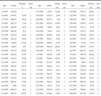
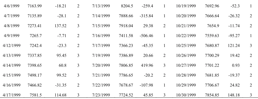
[Step 1] Calculate the fluctuation trend for each element in the historical training dataset of TAIEX1999. Then, use the whole mean of the fluctuation numbers of training dataset to fuzzify the fluctuation trends into FFTS as shown in Table I.
Table I Historical Training Data and Fuzzified fluctuation data of TAIEX1999
date TAIEX Fluctuatio n
fuzzif
ied date TAIEX
Fluctua
tion fuzzif
ied date TAIEX
Fluctuat
ion fuzzi
fied
1/5/1999 6152.43 - - 4/17/1999 7581.5 114.68 3 7/26/1999 7595.71 -128.81 1
1/6/1999 6199.91 47.48 3 4/19/1999 7623.18 41.68 2 7/27/1999 7367.97 -227.74 1
1/7/1999 6404.31 204.4 3 4/20/1999 7627.74 4.56 2 7/28/1999 7484.5 116.53 3
1/8/1999 6421.75 17.44 2 4/21/1999 7474.16 -153.58 1 7/29/1999 7359.37 -125.13 1
1/11/1999 6406.99 -14.76 2 4/22/1999 7494.6 20.44 2 7/30/1999 7413.11 53.74 3
1/12/1999 6363.89 -43.1 1 4/23/1999 7612.8 118.2 3 7/31/1999 7326.75 -86.36 1
1/13/1999 6319.34 -44.55 1 4/26/1999 7629.09 16.29 2 8/2/1999 7195.94 -130.81 1
1/14/1999 6241.32 -78.02 1 4/27/1999 7550.13 -78.96 1 8/3/1999 7175.19 -20.75 2
1/15/1999 6454.6 213.28 3 4/28/1999 7496.61 -53.52 1 8/4/1999 7110.8 -64.39 1
1/16/1999 6483.3 28.7 2 4/29/1999 7289.62 -206.99 1 8/5/1999 6959.73 -151.07 1
1/18/1999 6377.25 -106.05 1 4/30/1999 7371.17 81.55 3 8/6/1999 6823.52 -136.21 1
1/19/1999 6343.36 -33.89 2 5/3/1999 7383.26 12.09 2 8/7/1999 7049.74 226.22 3
1/20/1999 6310.71 -32.65 2 5/4/1999 7588.04 204.78 3 8/9/1999 7028.01 -21.73 2
1/21/1999 6332.2 21.49 2 5/5/1999 7572.16 -15.88 2 8/10/1999 7269.6 241.59 3
1/22/1999 6228.95 -103.25 1 5/6/1999 7560.05 -12.11 2 8/11/1999 7228.68 -40.92 2
1/25/1999 6033.21 -195.74 1 5/7/1999 7469.33 -90.72 1 8/12/1999 7330.24 101.56 3
1/26/1999 6115.64 82.43 3 5/10/1999 7484.37 15.04 2 8/13/1999 7626.05 295.81 3
1/27/1999 6138.87 23.23 2 5/11/1999 7474.45 -9.92 2 8/16/1999 8018.47 392.42 3
1/28/1999 6063.41 -75.46 1 5/12/1999 7448.41 -26.04 2 8/17/1999 8083.43 64.96 3
1/29/1999 5984 -79.41 1 5/13/1999 7416.2 -32.21 2 8/18/1999 7993.71 -89.72 1
1/30/1999 5998.32 14.32 2 5/14/1999 7592.53 176.33 3 8/19/1999 7964.67 -29.04 2
2/2/1999 5749.64 -113.15 1 5/17/1999 7599.76 23.12 2 8/21/1999 8153.57 36.15 2
2/3/1999 5743.86 -5.78 2 5/18/1999 7585.51 -14.25 2 8/23/1999 8119.98 -33.59 2
2/4/1999 5514.89 -228.97 1 5/19/1999 7614.6 29.09 2 8/24/1999 7984.39 -135.59 1
2/5/1999 5474.79 -40.1 2 5/20/1999 7608.88 -5.72 2 8/25/1999 8127.09 142.7 3
2/6/1999 5710.18 235.39 3 5/21/1999 7606.69 -2.19 2 8/26/1999 8097.57 -29.52 2
2/8/1999 5822.98 112.8 3 5/24/1999 7588.23 -18.46 2 8/27/1999 8053.97 -43.6 1
2/9/1999 5723.73 -99.25 1 5/25/1999 7417.03 -171.2 1 8/30/1999 8071.36 17.39 2
2/10/1999 5798 74.27 3 5/26/1999 7426.63 9.6 2 8/31/1999 8157.73 86.37 3
2/20/1999 6072.33 274.33 3 5/27/1999 7469.01 42.38 2 9/1/1999 8273.33 115.6 3
2/22/1999 6313.63 241.3 3 5/28/1999 7387.37 -81.64 1 9/2/1999 8226.15 -47.18 1
2/23/1999 6180.94 -132.69 1 5/29/1999 7419.7 32.33 2 9/3/1999 8073.97 -152.18 1
2/24/1999 6238.87 57.93 3 5/31/1999 7316.57 -103.13 1 9/4/1999 8065.11 -8.86 2
2/25/1999 6275.53 36.66 2 6/1/1999 7397.62 81.05 3 9/6/1999 8130.28 65.17 3
2/26/1999 6318.52 42.99 3 6/2/1999 7488.03 90.41 3 9/7/1999 7945.76 -184.52 1
3/1/1999 6312.25 -6.27 2 6/3/1999 7572.91 84.88 3 9/8/1999 7973.3 27.54 2
3/2/1999 6263.54 -48.71 1 6/4/1999 7590.44 17.53 2 9/9/1999 8025.02 51.72 3
3/3/1999 6403.14 139.6 3 6/5/1999 7639.3 48.86 3 9/10/1999 8161.46 136.44 3
3/4/1999 6393.74 -9.4 2 6/7/1999 7802.69 163.39 3 9/13/1999 8178.69 17.23 2
3/5/1999 6383.09 -10.65 2 6/8/1999 7892.13 89.44 3 9/14/1999 8092.02 -86.67 1
3/6/1999 6421.73 38.64 2 6/9/1999 7957.71 65.58 3 9/15/1999 7971.04 -120.98 1
3/8/1999 6431.96 10.23 2 6/10/1999 7996.76 39.05 2 9/16/1999 7968.9 -2.14 2
3/9/1999 6493.43 61.47 3 6/11/1999 7979.4 -17.36 2 9/17/1999 7916.92 -51.98 1
3/10/1999 6486.61 -6.82 2 6/14/1999 7973.58 -5.82 2 9/18/1999 8016.93 100.01 3
3/11/1999 6436.8 -49.81 1 6/15/1999 7960 -13.58 2 9/20/1999 7972.14 -44.79 1
3/12/1999 6462.73 25.93 2 6/16/1999 8059.02 99.02 3 9/27/1999 7759.93 -212.21 1
3/15/1999 6598.32 135.59 3 6/17/1999 8274.36 215.34 3 9/28/1999 7577.85 -182.08 1
3/16/1999 6672.23 73.91 3 6/21/1999 8413.48 139.12 3 9/29/1999 7615.45 37.6 2
3/17/1999 6757.07 84.84 3 6/22/1999 8608.91 195.43 3 9/30/1999 7598.79 -16.66 2
3/18/1999 6895.01 137.94 3 6/23/1999 8492.32 -116.59 1 10/1/1999 7694.99 96.2 3
3/19/1999 6997.29 102.28 3 6/24/1999 8589.31 96.99 3 10/2/1999 7659.55 -35.44 2
3/20/1999 6993.38 -3.91 2 6/25/1999 8265.96 -323.35 1 10/4/1999 7685.48 25.93 2
3/22/1999 7043.23 49.85 3 6/28/1999 8281.45 15.49 2 10/5/1999 7557.01 -128.47 1
3/23/1999 6945.48 -97.75 1 6/29/1999 8514.27 232.82 3 10/6/1999 7501.63 -55.38 1
3/24/1999 6889.42 -56.06 1 6/30/1999 8467.37 -46.9 1 10/7/1999 7612 110.37 3
3/25/1999 6941.38 51.96 3 7/2/1999 8572.09 104.72 3 10/8/1999 7552.98 -59.02 1
3/26/1999 7033.25 91.87 3 7/3/1999 8563.55 -8.54 2 10/11/1999 7607.11 54.13 3
3/29/1999 6901.68 -131.57 1 7/5/1999 8593.35 29.8 2 10/12/1999 7835.37 228.26 3
3/30/1999 6898.66 -3.02 2 7/6/1999 8454.49 -138.86 1 10/13/1999 7836.94 1.57 2
3/31/1999 6881.72 -16.94 2 7/7/1999 8470.07 15.58 2 10/14/1999 7879.91 42.97 3
4/1/1999 7018.68 136.96 3 7/8/1999 8592.43 122.36 3 10/15/1999 7819.09 -60.82 1
4/2/1999 7232.51 213.83 3 7/9/1999 8550.27 -42.16 2 10/16/1999 7829.39 10.3 2
4/6/1999 7163.99 -18.21 2 7/13/1999 8204.5 -259.4 1 10/19/1999 7692.96 -52.3 1
4/7/1999 7135.89 -28.1 2 7/14/1999 7888.66 -315.84 1 10/20/1999 7666.64 -26.32 2
4/8/1999 7273.41 137.52 3 7/15/1999 7918.04 29.38 2 10/21/1999 7654.9 -11.74 2
4/9/1999 7265.7 -7.71 2 7/16/1999 7411.58 -506.46 1 10/22/1999 7559.63 -95.27 1
4/12/1999 7242.4 -23.3 2 7/17/1999 7366.23 -45.35 1 10/25/1999 7680.87 121.24 3
4/13/1999 7337.85 95.45 3 7/19/1999 7386.89 20.66 2 10/26/1999 7700.29 19.42 2
4/14/1999 7398.65 60.8 3 7/20/1999 7806.85 419.96 3 10/27/1999 7701.22 0.93 2
4/15/1999 7498.17 99.52 3 7/21/1999 7786.65 -20.2 2 10/28/1999 7681.85 -19.37 2
4/16/1999 7466.82 -31.35 2 7/22/1999 7678.67 -107.98 1 10/29/1999 7706.67 24.82 2
4/17/1999 7581.5 114.68 3 7/23/1999 7724.52 45.85 3 10/30/1999 7854.85 148.18 3
[Step 2] Based on the FFTS from January 5, 1999 to October 30 shown in Table I, establish nth-order FFLRs for the forecasting model. For example, suppose n=6, following FFLRs of FFTS can be generated:
1 2 3 4 3 5 3 6 7
S(7)= 1.082 =
φ φ
+ +2 +2 +φ
φ
φ
+φ ε
+1 2 3 4 2 5 3 6 8
S(8)= 4.5091= + + +2 +
φ φ φ
φ
φ
+φ ε
+ (8)
1 2 3 4 5 6 221
2 2 2 3
S(221)= 3.7433 =
φ
+φ
+φ
+2 +φ
φ φ ε
+ +[Step 3] Replace each error
ε
tin Eq.(8) with one and the sameε
. Let the number of iterations itern=100, theinertia weight w=0.7298, self-confidence coefficient and social confidence coefficient c1=c2=1.4962, use
PSO algorithm listed in Fig.1 to determine the parameters
φ
k(k = 1,2,...,n) andε
. In the PSO process, eachelement in the generalized Eq.(8) is a particle and their personal best and global best positions are determined by the RMSE of actual values and forecast values. The obtained global best parameters are shown in Table II.
Table II Global Best Parameters Obtained Using PSO for Training Dataset
ϕ1 ϕ2 ϕ3 ϕ4 ϕ5 ϕ6 Ε RMSE
-0.1638 0.0803 0.1372 -0.0321 0.0433 0.2546 1.4408 115.73
[Step 4] Use the obtained global best parameters in Table II to forecast the test dataset from November 1, 1999 to December 30. For example, the forecasting value of the TAIEX on November 8, 1999, is calculated as follows:
Firstly, according to the fuzzy-fluctuation trends (2,1,1,1,2,1) and the parameters in Table II, the forecasted continuous labeled fuzzy-fluctuation number is :
2 (-0.1638)+0.0803+0.1372 - 0.0321+ 2 0.0433+0.2546 +1.4408 = 1.6398× ×
Then, the forecasted fluctuation from current value to next value can be obtained by defuzzify the fluctuation fuzzy number:
(1.6398 - 2) 85 = 30.62× −
Finally, the forecasted value can be obtained by current value and the fluctuation value:
7376.56 - 30.62 =7345.94
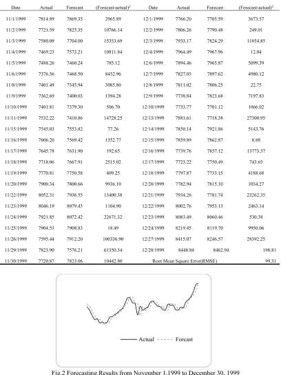
Table III Forecasting Results from November 1,1999 to December 30, 1999
Date Actual Forecast (Forecast-actual)2 Date Actual Forecast (Forecast-actual)2
11/1/1999 7814.89 7869.35 2965.89 12/1/1999 7766.20 7705.59 3673.57
11/2/1999 7721.59 7825.35 10766.14 12/2/1999 7806.26 7790.48 249.01
11/3/1999 7580.09 7704.00 15353.69 12/3/1999 7933.17 7824.29 11854.85
11/4/1999 7469.23 7573.21 10811.84 12/4/1999 7964.49 7967.96 12.04
11/5/1999 7488.26 7460.24 785.12 12/6/1999 7894.46 7965.87 5099.39
11/6/1999 7376.56 7468.50 8452.96 12/7/1999 7827.05 7897.62 4980.12
11/8/1999 7401.49 7345.94 3085.80 12/8/1999 7811.02 7806.25 22.75
11/9/1999 7362.69 7400.03 1394.28 12/9/1999 7738.84 7823.68 7197.83
11/10/1999 7401.81 7379.30 506.70 12/10/1999 7733.77 7701.12 1066.02
11/11/1999 7532.22 7410.86 14728.25 12/13/1999 7883.61 7718.38 27300.95
11/15/1999 7545.03 7553.82 77.26 12/14/1999 7850.14 7921.86 5143.76
11/16/1999 7606.20 7569.42 1352.77 12/15/1999 7859.89 7862.87 8.88
11/17/1999 7645.78 7631.90 192.65 12/16/1999 7739.76 7857.12 13773.37
11/18/1999 7718.06 7667.91 2515.02 12/17/1999 7723.22 7750.49 743.65
11/19/1999 7770.81 7750.58 409.25 12/18/1999 7797.87 7733.15 4188.68
11/20/1999 7900.34 7800.66 9936.10 12/20/1999 7782.94 7815.10 1034.27
11/22/1999 8052.31 7936.55 13400.38 12/21/1999 7934.26 7781.74 23262.35
11/23/1999 8046.19 8079.43 1104.90 12/22/1999 8002.76 7953.13 2463.14
11/24/1999 7921.85 8072.42 22671.32 12/23/1999 8083.49 8060.46 530.38
11/25/1999 7904.53 7908.83 18.49 12/24/1999 8219.45 8119.70 9950.06
11/26/1999 7595.44 7912.20 100336.90 12/27/1999 8415.07 8246.57 28392.25
11/29/1999 7823.90 7576.21 61350.34 12/28/1999 8448.84 8462.94 198.81
11/30/1999 7720.87 7823.06 10442.80 Root Mean Square Error(RMSE) 99.31
Fig.2 Forecasting Results from November 1,1999 to December 30, 1999
The forecasting performance can be assessed by comparing the difference between the forecasted values and the actual values. The widely indicators used in time series models comparisons are mean squared error (MSE), root of the mean squared error (RMSE), mean absolute error (MAE), mean percentage error (MPE), etc. These indicators are defined by Eqs. (9)–(12):
2
1
( ( ) ( ))
n
t
forecast t actual t MSE
n =
−
=
(9)2
1
( ( ) ( ))
n
t
forecast t actual t RMSE
n
= −
=
(10)1
( ( ) ( ))
n
t
forecast t actual t MAE
n =
−
=
(11)1
( ( ) ( )) / ( )
n
t
forecast t actual t actual t MPE
n =
−
=
(12)where n denotes the number of values forecasted, forecast(t) and actual(t) denote the predicted value and actual value at time t, respectively. As to the proposed method for 6th-order, the MSE, RMSE, MAE, MPE are 9862.33, 99.31, 75.22, 0.01, respectively.
In order to compare the forecasting results with different parameters such as the number n of the nth-order and the element number g of linguistic set used in the fluctuation fuzzifying process, different experiments under different parameters were carried out. Each kind of experiments was repeated 30 times. The forecasting errors of the averages for the experiments are shown in Table IV and Table V.
Table IV Comparison of Forecasting Errors for Different nth-order(g=3)
n 1 2 3 4 5 6 7 8 9 10
RMSE 109.04 105.47 103.04 102.96 101.92 99.12 99.59 99.6 98.75 99
Table V Comparison of Forecasting Errors for Different Linguistic Set (n=6)
G 3 5 7 none
RMSE 99.12 101.67 105.82 128.97
In table V, g=3 represents that the linguistic set is {Down, Equal, Up}, g=5 means {Greatly down, Slightly down, Equal, Slightly up, Greatly up}, g=7 means { Very Greatly down, Greatly down, Slightly down, Equal, Slightly up, Greatly up, Very Greatly up }, and "none" means that the fluctuation values won't be fuzzified at all.
From Table IV and Table V, we can see that the RMSEs are lower when n is equal to six or more. As to parameter g, obviously, fuzzified fluctuation trends perform better than none fuzzified ones, and it is proper to let g=3.
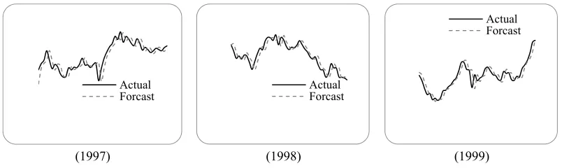
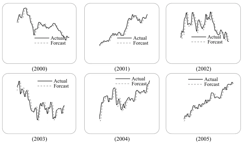
Let n=6 and g=3, employ the proposed method to forecast the TAIEX from 1997 to 2005. The forecasting results and errors are shown in Fig. 3 and Table VI.
(1997) (1998) (1999)
Actual
Forcast ActualForcast
(2000) (2001) (2002)
(2003) (2004) (2005)
Fig. 3. The stock market fluctuation for TAIEX test dataset(1997-2005)
Table VI RMSEs of forecast errors for TAIEX 1997 to 2005
Year 1997 1998 1999 2000 2001 2002 2003 2004 2005
RMSE 143.60 115.34 99.12 125.70 115.91 70.43 54.26 57.24 54.68
The following Table VII shows a comparison of RMSEs for different methods for forecasting TAIEX1999. From this table, we can see that the performance of proposed method is acceptable. The greatest advantage of the proposed method is that it put forward a method relying completely on machine learning mechanism. Though RMSEs of some of the other methods outperform the proposed method, they often need to determine complex discretization partitioning rules or use adaptive expectation model to justify the final forecasting results. The method proposed in this paper is more simply and easily to be realized by a computer program completely.
Table VII A Comparison of RMSEs for Different Methods for Forecasting TAIEX1999
Methods RMSE
Yu ‘s Method(2005)[29] 145
Hsieh et al. ‘s Method(2011)[17] 94
Chang et al. ‘s Method(2011)[2] 100
Cheng et al. ‘s Method(2013)[10] 103
Chen et al. ‘s Method(2013)[7] 102.11
Chen & Chen ‘s Method(2015) [5] 103.9
Chen & Chen ‘s Method(2015) [3] 92
Zhao et al. ‘s Method(2016)[30] 110.85
The Proposed Method 99.12
B. Forecasting SHSECI
The SHSECI (Shanghai Stock Exchange Composite Index) is the most famous stock market index in China. In the following, we apply the proposed method to forecast the SHSECI from 2007 to 2015. For each year, the authentic datasets of historical daily SHSECI closing prices from January to October are used as the training data, the datasets from November to December are used as the testing data. The forecasting results and the RMSEs of forecast errors are shown in Fig. 4 and Table VIII, respectively.
Actual
Forcast ActualForcast
Actual Forcast
Actual Forcast
Actual
(2007) (2008) (2009)
(2010) (2011) (2012)
(2013) (2014) (2015)
Fig. 4. The stock market fluctuation for SHSECI test dataset(2001-2015)
Table VIII RMSEs of forecast errors for SHSECI from 2007 to 2015
Year 2007 2008 2009 2010 2011 2012 2013 2014 2015
RMSE 113.11 55.28 49.59 45.73 28.45 25.05 19.86 41.44 59.5
From Fig.4. and Table VIII, we can see that the proposed method can successfully predict the stock market.
6. Conclusion
In this paper, a novel forecasting model is proposed based on high-order fuzzy-fluctuation logical trends and PSO machine learning method. The proposed method is based on the fluctuations of the time series. PSO method is employed to looking for the best parameters to minimize the RMSE for historical training dataset. Experiments shows that these parameters generated from training dataset can be successfully used for future dataset as well. In order to compare the performance with that of other methods, we take TAIEX1999 as an example. We also forecasted TAIEX1997-2005 and SHSECI 2007-2015 to verify its effectiveness and universality. In the future, we will consider other factors which might affect the fluctuation of the stock market, such as the
trade volume, the beginning value, the end value, etc. We also will consider the influence of other stock markets, such as the Dow Jones, the NASDAQ, the M1b and so on.
Acknowledgments: This work was supported by the National Natural Science Foundation of China under Grants (71471076), the Fund of Ministry of education of Humanities and Social Sciences (14YJAZH025), the Fund of China Nation Tourism Administration (15TACK003), the Natural Science Foundation of Shandong Province (ZR2013GM003) , and the Foundation program of Jiangsu University(16JDG005).
References
1. Askari S, Montazerin N (2015) A high-order multi-variate fuzzy times series forecasting algorithm based on fuzzy clustering, Expert Systems with Application 42: 2121-2135.
Actual Forcast
Actual Forcast
Actual Forcast
Actual
Forcast ActualForcast Actual
Forcast
Actual Forcast
Actual Forcast
2. Chang JR, Wei LY, Cheng CH (2011) A hybrid ANFIS model based on AR and volatility for TAIEX Forecasting, Appl. Soft Comput. 11:1388-1395.
3. Chen MY, Chen BT (2015) A hybrid fuzzy time series model based on granular computing for stock price forecasting, Information Science 294: 227-241.
4. Chen SM (1996) Forecasting enrollments based on fuzzy time series, Fuzzy Sets and Systems 81(3):311–319. 5. Chen SM, Chen SW (2015) Fuzzy forecasting based on two-factors second-order fuzzy-trend logical
relationship groups and the probabilities of trends of fuzzy logical relationships. IEEE Transaction on Cybernetics 45 (3): 405–417 .
6. Chen SM, Jian WS (2017) Fuzzy forecasting based on two-factors second-order fuzzy-trend logical relationship groups, similarity measures and PSO techniques, Information Sciences 391-392: 65-79. 7. Chen SM, Manalu GMT, Pan JS, Liu HC (2013) Fuzzy forecasting based on two-factors second-order
fuzzy-trend logical relationship groups and particle swarm optimization techniques, IEEE Trans. Cybern. 43(3): 1102–1117.
8. Chen SM, Wang NY (2010) Fuzzy forecasting based on fuzzy-trend logical relationship groups, IEEE Transactions on Systems Man & Cybernetics Part B Cybernetics A Publication of the IEEE Systems Man & Cybernetics Society 40(5):1343-1358.
9. Cheng CH, Chen TL, Teoh HJ, Chiang CH (2008) Fuzzy time-series based on adaptive expectation model for TAIEX forecasting, Expert Syst. Appl. 34 (2): 1126–1132.
10. Cheng CH, Wei LY, Liu JW, Chen TL (2013) OWA-based ANFIS model for TAIEX forecasting, Econ. Model. 30: 442–448.
11. Cheng H, Chang RJ,Yeh CA (2006) Entropy-based and trapezoid fuzzification based fuzzy time series approach for forecasting it project cost, Technological Forecasting and Social Change 73(5):524–542. 12. Cheng S, Shi Y, Qin Q (2011) Experimental study on boundary constraints handling in particle swarm
optimization: from population diversity perspective, International Journal of Swarm Intelligence Research 2(3): 43-69.
13. Efendi R, Ismail Z, Deris MM (2015) A new linguistic out-sample approach of fuzzy time series for daily forecasting of Malaysian electricity load demand, Applied Soft Computing 28:422-430.
14. Gangwar SS, Kumar S (2012) Partitions based computational method for high-order fuzzy time series forecasting, Expert Systems with Applications 39(15): 12158-12164.
15. Herrera F, Herrera-Viedma E, Verdegay JL (1996) A model of consensus in group decision making under linguistic assessments, Fuzzy Sets and Systems 79: 73-87.
16. Huarng KH(2010) Effective lengths of intervals to improve forecasting in fuzzy time series, Fuzzy sets and Systems 123: 387-394.
17. Hsieh TJ, Hsiao HF, Yeh WC (2011) Forecasting stock markets using wavelet trans-forms and recurrent neural networks: An integrated system based on artificial bee colony algorithm, Applied Soft Computing 11:2510–2525.
18. Kennedy J, Eberhart R 2011) Particle swarm optimization. Springer, New York.
19. Lahrimi S (2016a) Intraday stock prime forecasting based on variational mode decomposition, Journal of Computational Science 12: 23-27.
20. Lahrimi S (2016b) A variational mode decomposition approach for analysis and forecasting of economic and financial time series, Expert Systems with Application 55: 268-276.
21. Rubio A, Bermudez JD, Vercher E(2017) Improving stock index forecasts by using a new weighted fuzzy-trend time series method, Expert Systems With Applications 76:12-20.
22. Sadaei HJ, Guimaraes FG, Silva CJ, Lee MH, Eslami T (2017) Short-term load forecasting method based on fuzzy time series, seasonality and long memory process. International Journal of Approximate Reasoning 83: 196-217.
23. Schutte JF, Reinbolt JA, Fregly BJ, Haftka RT, George AD (2004) Parallel global optimization with the particle swarm algorithm, Communications in Numerical Methods in Engineering 61(13): 2296-2315. 24. Singh SR(2009) A computational method of forecasting based on high-order fuzzy time series, Expert
Systems with Applications 36 (7): 10551-10559.
25. Song Q, Chissom BS (1993) Forecasting enrollments with fuzzy time series—Part I, Fuzzy Sets Syst. 54(1): 1–9.
27. Song Q, Chissom BS (1994) Forecasting enrollments with fuzzy time series—Part II, Fuzzy Sets Syst. 62(1):1–8.
28. Wang L, Liu X, Pedrycz W (2013) Effective intervals determined by information granules to improve forecasting in fuzzy time series, Expert Systems with Application 40: 5673-5679.
29. Yu HK(2005). Weighted fuzzy time series models for TAIEX forecasting, Physica A, 349 (3–4): 609–624. 30. Zhao AW, Guan S, Guan HJ (2016) A computational fuzzy time series forecasting model based on