Actuator Networks
Article
Enhanced Distributed Dynamic Skyline Query for
Wireless Sensor Networks
Khandakar Ahmed1,2,3,*, Nazmus S. Nafi4,†and Mark A. Gregory4,†
1 School of Electrical and Computer Engineering, RMIT University, Melbourne, VIC 3000, Australia 2 Melbourne Institute of Technology, Melbourne VIC 3000, Australia
3 Department of Computer Science & Engineering, Shahjalal University of Science & Technology, Sylhet-3114, Bangladesh
4 School of Electrical and Computer Engineering, RMIT University, Melbourne, VIC 3000, Australia; [email protected] (N.S.N.); [email protected] (M.A.G.)
* Correspondence: [email protected] or [email protected] or [email protected]; Tel.: +61-3-9925-1180 (ext. 51180)
† These authors contributed equally to this work.
Academic Editor: Stefan Fischer
Received: 16 November 2015; Accepted: 28 January 2016; Published: 3 February 2016
Abstract:Dynamic skyline query is one of the most popular and significant variants of skyline query in the field of multi-criteria decision-making. However, designing a distributed dynamic skyline query possesses greater challenge, especially for the distributed data centric storage within wireless sensor networks (WSNs). In this paper, a novel Enhanced Distributed Dynamic Skyline (EDDS) approach is proposed and implemented in Disk Based Data Centric Storage (DBDCS) architecture. DBDCS is an adaptation of magnetic disk storage platter consisting tracks and sectors. In DBDCS, the disc track and sector analogy is used to map data locations. A distance based indexing method is used for storing and querying multi-dimensional similar data. EDDS applies a threshold based hierarchical approach, which uses temporal correlation among sectors and sector segments to calculate a dynamic skyline. The efficiency and effectiveness of EDDS has been evaluated in terms of latency, energy consumption and accuracy through a simulation model developed in Castalia.
Keywords: wireless sensor networks; distributed data centric storage; skyline query; sector based distance routing; uniform distribution; lower bound distribution; and upper bound distribution
1. Introduction
WSNs have successfully been validated as a very economic and effective platform for monitoring diverse physical environments from remote locations. Various types of query techniques have been developed over WSNs including min-max [1], top-k [2,3] and skyline [4]. Skyline and its variants such astraditional skyline[5] anddynamic skyline[6–8] have been applied in many multiple criteria decision making applications. Traditional skyline(TS) retrieves all of the points, which are not dominated by others, from a set of points [9]. Given a datasetX, a pointx1dominatesx2, ifx1is not worse than x2 for each dimensioni P l (i.e., x1[i]ďx2[i]), andx1is better thanx2for at least one dimension mPl(x1[m]< x2[m]). Figure1a shows an example, where each point is drawn taking two dimensionsi andjas coordinators; pointsx1,x3,x6andx10are in the skyline set considering that a point with the least value for each dimension is desirable.
Dynamic skyline(DS) retrieves a set of points that are not dynamically dominated by others with respect to a data pointqdenoted by DS (q, X)) [10]. A pointx1dynamically dominatesx2with respect toqif for each dimension iniP l,|x1ris ´qris| ď |x2ris ´qris|and for at least one dimension inmPl,
|x1rms ´qrms| ă |x2rms ´qrms|. In Figure1b, pointsx1,x2andx4are the dynamic skyline points ofq. Each pointxi= (xi[j],xi[i]) is transformed toxi1= (xi[j]´q[j],xi[i]´q[i]).
m qm x
m qmx1 2 . In Figure 1b, points x1, x2 and x4 are the dynamic skyline points of q. Each
point xi = (xi[j], xi[i]) is transformed to xi′ = (xi[j]-q[j], xi[i]-q[i]).
j
i
x
1x
10x
3x
6x
5x
7x
4x
8x
9j
i
x
1x
10
x
3x
6x
5x
7x
2x
8x
9X
4'X
1'q
X
2'X
4X
6'x
2(a) (b)
Figure 1. (a) TS and (b) DS (q, X).
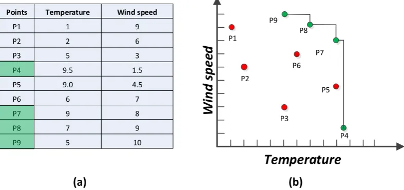
Skyline query is very useful in multi-preference analysis and decision making for environmental monitoring applications. For example, in a WSN deployed in a forest with each sensor node sensing temperature and wind speed, it is possible to build a fast and energy efficient forest fire detection method [11] by concentrating on places with high temperature or fast wind speed, or both. To illustrate the idea of dominance relations in this scenario, consider the readings in the two-dimensional attribute space shown in Figure 2 depicting a typical example of ranking objects by more than one criterion. Figure 2a lists nine records received from nine corresponding sensor nodes deployed in different places and their values. Figure 2b depicts the representation in a 2D space. Places P1, P2, P3, P5, and P6 are all dominated by other points so the skyline query returns the points
that are not dominated by any other points. Consider the point P5 that is dominated by P7, as it has a
higher wind speed than P5 though both have the same temperature. The skyline query only retrieves
the dominant places in terms of higher temperature and wind speed. The skyline query will not exhibit any place with lower temperature and wind speed once it is dominated by a location with higher values. Therefore, the result set of the skyline query consists of {P4, P7, P8, P9}, which are
indicators of dangerous places that need special attention.
Temperature
W
in
d
sp
ee
d
Points P1 P2 P3 P4 P5 P6 P7 P8 P9 Wind speed 9 6 3 1.5 4.5 7 8 9 10 Temperature 1 2 5 9.5 9.0 6 9 7 5 P6 P4 P1 P2 P3 P5 P7 P8 P9(a)
(b)
Figure 2. (a) Skyline of sensor readings, (b) Representation of sensor readings in 2D space [11].
Another example that demonstrates the usefulness of DS can be found when monitoring the air pollution in a region of interest. A high concentration of CO or SO2, or both, can be a strong indication
Figure 1.(a) TS and (b) DS (q, X).
Skyline query is very useful in multi-preference analysis and decision making for environmental monitoring applications. For example, in a WSN deployed in a forest with each sensor node sensing temperature and wind speed, it is possible to build a fast and energy efficient forest fire detection method [11] by concentrating on places with high temperature or fast wind speed, or both. To illustrate the idea of dominance relations in this scenario, consider the readings in the two-dimensional attribute space shown in Figure2depicting a typical example of ranking objects by more than one criterion. Figure2a lists nine records received from nine corresponding sensor nodes deployed in different places and their values. Figure2b depicts the representation in a 2D space. Places P1, P2, P3, P5, and P6are all dominated by other points so the skyline query returns the points that are not dominated by any other points. Consider the point P5that is dominated by P7, as it has a higher wind speed than P5 though both have the same temperature. The skyline query only retrieves the dominant places in terms of higher temperature and wind speed. The skyline query will not exhibit any place with lower temperature and wind speed once it is dominated by a location with higher values. Therefore, the result set of the skyline query consists of {P4, P7, P8, P9}, which are indicators of dangerous places that need special attention.
m qm x
m qmx1 2 . In Figure 1b, points x1, x2 and x4 are the dynamic skyline points of q. Each
point xi = (xi[j], xi[i]) is transformed to xi′ = (xi[j]-q[j], xi[i]-q[i]).
j
i
x
1x
10x
3x
6x
5x
7x
4x
8x
9j
i
x
1x
10
x
3x
6x
5x
7x
2x
8x
9X
4'X
1'q
X
2'X
4X
6'x
2(a) (b)
Figure 1. (a) TS and (b) DS (q, X).
Skyline query is very useful in multi-preference analysis and decision making for environmental monitoring applications. For example, in a WSN deployed in a forest with each sensor node sensing temperature and wind speed, it is possible to build a fast and energy efficient forest fire detection method [11] by concentrating on places with high temperature or fast wind speed, or both. To illustrate the idea of dominance relations in this scenario, consider the readings in the two-dimensional attribute space shown in Figure 2 depicting a typical example of ranking objects by more than one criterion. Figure 2a lists nine records received from nine corresponding sensor nodes deployed in different places and their values. Figure 2b depicts the representation in a 2D space. Places P1, P2, P3, P5, and P6 are all dominated by other points so the skyline query returns the points
that are not dominated by any other points. Consider the point P5 that is dominated by P7, as it has a
higher wind speed than P5 though both have the same temperature. The skyline query only retrieves
the dominant places in terms of higher temperature and wind speed. The skyline query will not exhibit any place with lower temperature and wind speed once it is dominated by a location with higher values. Therefore, the result set of the skyline query consists of {P4, P7, P8, P9}, which are
indicators of dangerous places that need special attention.
Temperature
W
in
d
sp
ee
d
Points P1 P2 P3 P4 P5 P6 P7 P8 P9 Wind speed 9 6 3 1.5 4.5 7 8 9 10 Temperature 1 2 5 9.5 9.0 6 9 7 5 P6 P4 P1 P2 P3 P5 P7 P8 P9(a)
(b)
Figure 2. (a) Skyline of sensor readings, (b) Representation of sensor readings in 2D space [11].
Another example that demonstrates the usefulness of DS can be found when monitoring the air pollution in a region of interest. A high concentration of CO or SO2, or both, can be a strong indication
Another example that demonstrates the usefulness of DS can be found when monitoring the air pollution in a region of interest. A high concentration of CO or SO2, or both, can be a strong indication that the location is highly polluted. An environmental scientist can issue a dynamic skyline query for CO and SO2levels to monitor the air pollution surrounding a particular region of interest.
DS query processing over moving objects is also very useful for numerous applications, such as location-aware computing, object tracking and monitoring, virtual environments, uncertain data stream, computer games, visualization,etc.
Although the skyline query approach has potential for use in WSN applications, it faces challenges because of high processing complexity and cost related with updating the results. The main contributors to the high cost are the data access cost from storage locations and the processing cost while executing the user specified query for a dominance check. It is important to note that search efficiency and update criteria are two key requirements of skyline query processing and skyline result maintenance.
Data-Centric Storage (DCS) [12,13], an alternate to External Storage (ES) and Local Storage (LS), is considered to be a promising and efficient storage and search mechanism. There has been a growing interest in understanding and optimizing WSN DCS schemes in recent years, where a various number of query mechanisms such as point query, range query, similarity searching, top-k query and skyline query can be applied in a consolidated framework. As part of developing such consolidated framework, this paper proposes a threshold based hierarchical approach, which uses temporal correlation among the sectors and sector segments to calculate DS in a region of interest. To our knowledge, this is the first practical demonstration of DS in DCS of WSN in current state-of-the-art.
In this paper, first a novel tree building algorithm is incorporated so that each head node of a cluster could construct a tree with itself as a root. This allows exertion of three core operations such asTree Propagation,Regular UpdateandTriggered Queryfrom any head node with a particular range. The performance of the proposed model is analyzed by framing and implementing it in a distributed information delivery service running one or more applications in a WSN. In this service, a set of producer and consumer nodes exchange information by relaying packets through neighboring clusters for each application. This phenomenon is facilitated by a DCS [14] architecture, also referred to as DBDCS (Section3.1). DBDCS is an adaptation of the magnetic disk storage platter consisting of tracks and sectors [15,16]. In DBDCS, each application uses a disc track and sector analogy to map data locations and uses distance based indexing method for storing and querying multi-dimensional similar data. The member nodes in each cluster report the sensed event to their associated head node, which aggregates the received events at the end of each epoch. The aggregated event is hashed to produce a hash key, which is mapped from a one dimensional domain into a metric space [17] (Section3.3).
The remainder of this paper is structured as follows: Section2provides an overview of the related work in the literature. Network architecture, data processing and mapping, insertion and skyline querying are illustrated in Section3. This is followed by the simulation results and performance evaluation of EDDS presented in Section4. The paper is concluded in Section5.
2. Related Work
A filter-based distributed algorithm for skyline evaluation and maintenance in WSN is proposed by Lianget al.[23]. Each sensor node uses a greedy algorithm to compute a local skyline certificate, which is a subset of the local skyline and forwards it to its parent. The parent or non-leaf node calculates the certificate based on a set of local skyline points plus the certificate received from child nodes. Following this process, the root calculates the set of skyline points, which is used as a Global Skyline Filter (GSF) or global certificate. The root broadcasts the global certificate followed by a simple merge-based algorithm to filter out the points from transmissions that cannot utilize the certificate. An energy efficient Sliding Window Skyline Monitoring Algorithm (SWSMA) is proposed in [24] to continuously maintain sliding window skylines over WSN. It reduces the amount of data transferred and reduces energy consumption, as a consequence, by devising two filter based algorithms: (1) Single point filter based algorithm referred to as a Tuple Filter (TF); and (2) Grid Filter (GF) based algorithm. Chenet al.[25] proposed two evaluation algorithms for finding the skyline points on a dataset progressively. The dataset is first partitioned into disjoint subsets. Then skyline points are returned through the examination of each subset progressively using discovered skyline points to filter out the unlikely skyline points from transmission. However, the features of DCS have not been considered in these approaches and thus direct implication of them in DCS is not suitable.
Songet al.[26] propose a skyline query processing algorithm exploiting the key features of DCS. The algorithm processes a query in three stages on the basis of four assumptions: (1) choice of DCS framework is limited to KDDCS [27], GDCS [28] and DIM [29]; (2) all nodes are identified by unique ID; (3) each node knows the geographic location of its own and its neighbor nodes; and (4) each node knows the range of data stored in its neighbor nodes. In the first stage, the base station locates the Start Node (SN) where the query is to commence. In the second stage, SN creates a Skyline Query Message (SQM) and propagates the SQM to neighbor nodes to search for Candidate Nodes (CNs) where candidate data for the query are stored. This SQM transmission process is repeated until the complete candidate results are found. In the third and final stage BS generates a final query result from its gathered candidate dataset. The aforementioned assumptions made in this work are particularly expensive in a distributed environment like WSN especially DCS framework.
Su et al.[30] proposed an algorithm, known as Skyline Sensor Algorithm (SkySensor), in a customized DCS method in order to collect and store all sensor readings and retrieve skyline results efficiently from the network. The major disadvantages of SkySensor are: (1) SkySensor needs increased effort from an application designer who has to write the center location of each cluster in such a way that no two clusters overlap; (2) number of clusters in a sensor network depends on the number of attributes of a tuple, therefore, an active sensor and actuator network, with higher rate of data generation and a lower number of attributes leads to high concentration of data in a small portion of the network which creates congestion and a hot spot around the cluster and limits the ultimate goal or advantage of DCS; and (3) in the case of resilience to node failure, an inefficient and old technique referred to as local replication is used, which is expected to incur high storage cost and increased data loss during a node group failure.
Based on the above discussion, it is obvious that none of the work from the current literature has implemented DS in WSN, especially in DCS. It consumes great effort in pre-processing, such as gathering the local skylines of all sensors, mapping all detected data of the entire network (both inflow and outflow). The overall process is overwhelmed with higher overheads and complexity if the researcher or analysts are interested in a particular region. In this paper, a threshold based hierarchical DS approach is proposed and implemented using the temporal correlation among the sectors and sector segments. This allows reducing the transmission cost in a greater aspect and facilitates finding skyline points from both entire network and a particular region of interest.
3. Basic System Design
metric based searching. This is followed by the discussion of data processing, mapping and insertion technique in Sections3.3and3.4. Finally, we have presented the EDDS approach in Section3.5.
3.1. Network Architecture
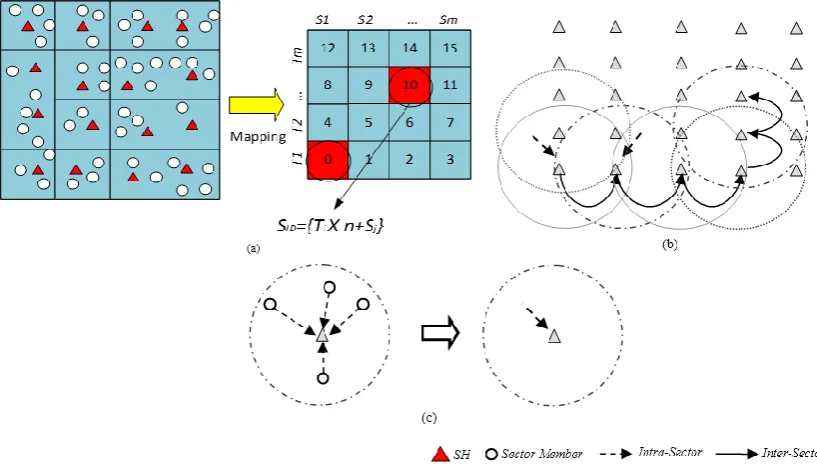
The surface/platter of a magnetic disk storage device consisting of tracks and sectors provides an interesting approach that may be applied to a large scale WSN. This assumption led to the Disk Based Data Centric Storage (DBDCS) architecture, as shown in Figure3a, dividing the rectangular field into a matrix of storage cells (referred to as a sector) where row and column represent trackTiand sectorSj, respectively. The physical deployment is mapped to am x nmatrix, wheremis the number of tracks andnis the number sectors for each track. Hence, the nodes in the network are divided intoS(mxn) sectors, each comprising a Sector Head (SH) and sector members that communicate via one hop to the SH (see Figure3c), whereSHi P r1..Ss. Each node is configured to be aware of the deployment layout by knowing: (1) each SH is assigned with the sector number as a virtual address and node id; and (2) all member nodes know their own node id and number of tracks (m) and sectors (n) of the network field. As shown in Figure3b, the intra-sector communication (i.e., communication from sector members toSHorvice-versa) is constrained to one hop while inter-sector transmission is multi-hop. For simplification, the sensor nodes inside each sector are not shown explicitly in Figure3b. Instead, an aggregated link (see Figure3c) is shown to represent the total traffic from member nodes to head node.
J. Sens. Actuator Netw. 2016, 5, 2 5 of 21
and sector Sj, respectively. The physical deployment is mapped to a m x n matrix, where m is the
number of tracks and n is the number sectors for each track. Hence, the nodes in the network are divided into S(mxn) sectors, each comprising a Sector Head (SH) and sector members that communicate via one hop to the SH (see Figure 3c), whereSHi
1..S . Each node is configured to be aware of the deployment layout by knowing: (1) each SH is assigned with the sector number as a virtual address and node id; and (2) all member nodes know their own node id and number of tracks (m) and sectors (n) of the network field. As shown in Figure 3b, the intra-sector communication (i.e., communication from sector members to SH or vice-versa) is constrained to one hop while inter-sector transmission is multi-hop. For simplification, the sensor nodes inside each sector are not shown explicitly in Figure 3b. Instead, an aggregated link (see Figure 3c) is shown to represent the total traffic from member nodes to head node.Figure 3. (a) DBDCS Mapping; (b) inter-sector communication; and (c) intra-sector member node to
head node communication
3.2. Skyline Definition with Metric-Based Searching
Metric space M can be defined as a pair M = (D, d), where D is the domain of objects and d is the
distance function—d:D × D R satisfying the following constraints (Equation (1)) for all objectsa,b,cD:
a,b 0d (non-negativity)
(1)
a,b 0d (identity)
) , ( ) ,
(ab d ba
d (symmetry)
) , ( ) , ( ) ,
(ac d ab d bc
d (triangle inequality)
In this metric space, considering that smaller values are preferable to larger ones for a set of l -dimensional data, the dynamic skyline query result set can be defined as:
Skyline(q, r):
X
=
"
iÎ
[ ]
1,
l
,
a
,
b
Î
I
|
a
(
i
)
£
b
(
i
)
and
$
iÎ
[1,
l
],
a
(
i
)
<
b
(
i
)
and
d q
( )
,
a
£
r
ì
í
ïï
î
ï
ï
ü
ý
ïï
þ
ï
ï
(2) Figure 3.(a) DBDCS Mapping; (b) inter-sector communication; and (c) intra-sector member node to head node communication
3.2. Skyline Definition with Metric-Based Searching
Metric spaceMcan be defined as a pairM= (D,d), whereDis the domain of objects anddis thedistance function—d: DˆDÔRsatisfying the following constraints (Equation (1)) for all objects a,b,cP D:
dpa,bq ě0 pnon´negativityq dpa,bq “0 pidentityq
dpa,bq “dpb,aq psymmetryq
dpa,cq ďdpa,bq `dpb,cq ptriangle inequalityq
(1)
Skyline(q, r): X“ $ ’ & ’ %
@iP r1,ls,a,bPI|apiq ďbpiqand DiP r1,ls,apiq ăbpiqand
dpq,aq ďr
, / . / -(2)
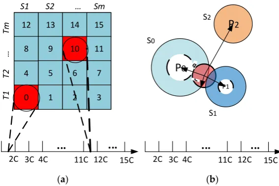
In Equation (2),qdenotes the query point,a(i)denotes the value of theithattribute of an object andrdefines the range of the region of interest. The data space is divided intoSsectors with a pivot point, denoted byPi, for each sectorSi. TheiDistancekey for an object x P Dcan be defined as (Figure4a, Equation (3)):
iDistpxq “dpPi,xq `i¨c (3)
In Equation (3),cis the separating constant for individual sectors. GivenqP D, the region of interest with radiusrcan be defined as (Figure4b, Equation (4)):
r“ rdpPi,qq `i¨c´r,dpPi,qq `i¨c`rs (4)
J. Sens. Actuator Netw. 2016, 5, 2 6 of 21
In Equation (2), q denotes the query point, a(i)denotes the value of the ith attribute of an object and r defines the range of the region of interest.The data space is divided into S sectors with a pivot point, denoted by Pi, for each sector Si. The iDistance key for an object xD can be defined as (Figure 4a, Equation (3)):
x d
P x
i ciDist i, (3)
In Equation (3), c is the separating constant for individual sectors. GivenqD, the region of interest with radius r can be defined as (Figure 4b, Equation (4)):
r
=
éë
d P
( )
i,
q
+
i
×
c
-
r
,
d P
( )
i,
q
+
i
×
c
+
r
ùû
(4)12 13 14 15
8 9 10 11
4
0
5 6 7
1 2 3
T1 T2 T m
S1 S2 Sm
P
2P
0 S0S2
S1
2C 3C 4C
...
...
11C 12C 15C 2C 3C 4C 11C 12C 15C
...
...
(a) (b)
Figure 4. (a) Data mapping; and (b) range query example.
3.3. Data Processing and Mapping
A sensed event E can be defined by an l- dimensional tuple, (A1, A2, A3, … Al) where Ag,g
1,l denotes the gth attribute and DAg is the domain of attribute Ag. Each member node of a sectortransmits the sensed event as an l-tuple vi1,vi2,...,vil k, where1iMk, Mkis the total number of member nodes in kth sector and vij denotes the value of the jth attribute received from ith node of kth sector. A SH node after collecting tuples from all the member nodes aggregates them at the end of each epoch before finding the mapping for the target SH.
Hence, after aggregation at epoch t
k M il ii v v t
v
1 i Agg 1 2
k(Agg(t)) , ,...,
E (5.1)
tl
1, 2,...,
(5.2)
Here,
kv k v avgMk
j
l k Si ij M i ij M i
j max1 ,min1 , 1 , 1, , 1,
(6)In Equation (6), Mkdenotes the number of member nodes in kth sector. It is assumed that all attribute’s aggregated values of
i have been normalized to be between 0 and 1. As shown in Table 1, weights have been assigned to different attributes based on their importance in the eventFigure 4.(a) Data mapping; and (b) range query example.
3.3. Data Processing and Mapping
A sensed eventEcan be defined by anl- dimensional tuple, (A1, A2, A3,. . .Al) whereAg,@gP r1,ls denotes thegth attribute andDAgis the domain of attributeAg. Each member node of a sector transmits the sensed event as anl-tuplexvi1,vi2, ...,vilyk, where 1ďiďMk,Mkis the total number of member nodes inkthsector andvijdenotes the value of thejthattribute received fromithnode ofkthsector. ASHnode after collecting tuples from all the member nodes aggregates them at the end of each epoch before finding the mapping for the targetSH.
Hence, after aggregation at epocht
EkpAggptqq “ Mk ż
Aggi“1
xvi1,vi2, ...,vily ptq (5.1)
“ xψ1,ψ2, ...,ψly ptq (5.2)
Here,
ψj“
!
maxMk
i“1vij, minMi“k1vij,avgMi“k1
)
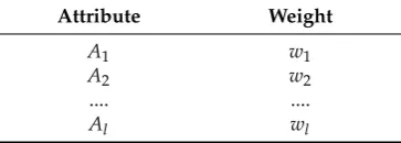
In Equation (6),Mkdenotes the number of member nodes inkthsector. It is assumed that all attribute’s aggregated values ofψihave been normalized to be between 0 and 1. As shown in Table1, weights have been assigned to different attributes based on their importance in the event description. Hence, an attribute with higher weight has higher influence in deciding the similarity among events.
Table 1.Weight settings.
Attribute Weight
A1 w1
A2 w2
.... ....
Al wl
3.3.1. Pivot Point Generation
αmin“ l
ÿ
i“1
´´
Aipminq{Aipmaxq
¯
ˆwi
¯
(7.1)
αmax“ l
ÿ
i“1
´´
Aipmaxq{Aipmaxq
¯
ˆwi
¯
(7.2)
β“ l
ÿ
i“1
´´
Aipavgq{Aipmaxq
¯
ˆwi
¯
(7.3)
δ“ l
ÿ
i“1
´´
Aipθq{Aipmaxq
¯
ˆwi¯ (7.4)
In Equations (7.1)–(7.4), Ai(min), Ai(max), Ai(avg)and Aipθqdenote the minimum, maximum, average
and threshold value ofithattribute. Based on Equations (7.1) and (7.2), the domain of the hash key, denoted byHD, isα(αmin,αmax). The center of gravity, denoted byβ, is derived in Equation (7.3) to find the normalized center point of the domain of the hash keyHD, whereasδis the separating factor between two pivot points. However, in order to balance the load among sectors, it is important to find the range where the concentration of the data points is high. Hence,βandδcan be used to find the range for center of gravity, denoted byβ(βrange´min,βrange´max), as shown in Equation (8).
βrange´min“β´δ
βrange´max“β`δ (8)
Thus, the separating step, denoted by η, between two pivot points in COM range can be defined by:
η“`βrange´max´βrange´min
˘
{S´1 (9)
Thus, the pivot points forSsectors can be defined in each sector head by:
Pi“
$ ’ &
’ %
αmin,
βrange´min`iˆη, αmax,
i“0 0ăiăS i“S
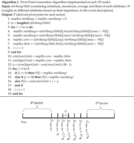
Algorithm 1. Pivot Point Generation Algorithm (implemented at eachSHnode).
Input:attrRangeTable(containing minimum, maximum, average and theta of each attribute),W (weights to different attributes based on their importance in the event description).
Output:P (derived pivot point for each sector) 1:mapRec.minRange=mapRec.maxRange= 0 2:m=lengthof(attrRangeTable)
3:fori= 1 tomdo
4: mapRec.minRange+=(attrRangeTable[i].min/attrRangeTable[i].max)ˆW[i] 5: mapRec.maxRange+=(attrRangeTable[i].max)/attrRangeTable[i].max)ˆW[i] 6: mapRec.com+= (attrRangeTable[i].avg)/attrRangeTable[i].max)ˆW[i] 7: mapRec.theta += (attrRangeTable.theta)/attrRangeTable[i].max)ˆW[i] 8: i=i+ 1
9:end for
10:comLowerLimit=mapRec.com-mapRec.theta 11:comUpperLimit=mapRec.com+mapRec.theta 12:η= (comUpperLimit-comLowerLimit)/(S- 1) 13:forj= 0 toS
14: if(j== 0)thenP[j]=mapRec.minRange 15: else if(j==S) thenP[j] = mapRec.maxRange 16: elseP[j] = comLowerLimit+jˆη
17: end if
18: j=j+ 1 19:end for
J. Sens. Actuator Netw. 2016, 5, 2 8 of 21
5: mapRec.maxRange+=(attrRangeTable[i].max)/attrRangeTable[i].max)× W[i] 6: mapRec.com += (attrRangeTable[i].avg)/attrRangeTable[i].max) × W[i] 7: mapRec.theta += (attrRangeTable.theta)/attrRangeTable[i].max) × W[i] 8: i = i + 1
9: end for
10: comLowerLimit = mapRec.com - mapRec.theta
11: comUpperLimit = mapRec.com + mapRec.theta
12: η = (comUpperLimit - comLowerLimit)/(S - 1)
13: forj = 0 to S
14: if (j == 0) thenP[j] = mapRec.minRange
15: else if (j == S)thenP[j] = mapRec.maxRange
16: else P[j] = comLowerLimit + j × η
17: end if
18: j = j + 1
19: end for
Figure 5. Pivot point generation example.
Algorithm 1 uses Equations (8)–(10) for calculating pivot points. Figure 5 illustrates the domain and sub-domain of pivot points.
3.3.2. Mapping
Given l attributes in an attribute list associated with weight wj (1 ≤ j ≤ l) in a WSN application, the source SHk generates the hash value by:
l
j ij j j
M
i
v
A
w
avg
h
k1 1 (max) (11)
Hence, after each epoch, SHk forwards the aggregated eventEk
1,
2,,
l
,t,h , where t denotes the epoch number, to the destination sector head denoted by SHi where, PihPi1and Pi and Pi+1 is the lower and upper limit of ith sub-interval, respectively.3.4. Insertion
Within a sector, data are further distributed among nodes according to their distance from the SH. In order to do so, a sector is divided into segments. Figures 6 and 7 and Table 2 illustrate the idea of sector segmentation. Given a kth sector containing Mk member nodes, the SHk first sorts all member nodes based on RSSI in ascending order. The member nodes are then divided into r segments. Each segment forms a circle, denoted by B(X,Y) (ri), where the center of the circle is (X, Y) with radius ri. (X, Y) is the geographic co-ordinates for SHk. The number of segments depends on the WSN application, sector size and the number of member nodes in each sector. Thus the set of sensors that are within a Euclidean distance ri from (X, Y) form the segment defined by:
Figure 5.Pivot point generation example.
Algorithm 1 uses Equations (8)–(10) for calculating pivot points. Figure5illustrates the domain and sub-domain of pivot points.
3.3.2. Mapping
Givenlattributes in an attribute list associated with weightwj(1ďjďl) in a WSN application, the sourceSHkgenerates the hash value by:
h“ l
ÿ
j“1
´´
avgMk
i“1vij{Ajpmaxq
¯
ˆwj
¯
(11)
3.4. Insertion
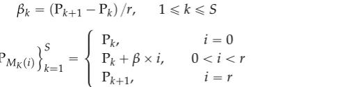
Within a sector, data are further distributed among nodes according to their distance from the SH. In order to do so, a sector is divided into segments. Figures6and7and Table2illustrate the idea of sector segmentation. Given akthsector containingMkmember nodes, theSHkfirst sorts all member nodes based on RSSI in ascending order. The member nodes are then divided intorsegments. Each segment forms a circle, denoted byBpX,Yq(ri), where the center of the circle is (X, Y) with radius ri. (X, Y) is the geographic co-ordinates forSHk. The number of segments depends on the WSN application, sector size and the number of member nodes in each sector. Thus the set of sensors that are within a Euclidean distancerifrom (X, Y) form the segment defined by:
BpX,Yqpriq “ tSensorsCoordinatepx,yq:|pX,Yq,px,yq| ďriu (12)
βk“ pPk`1´Pkq {r, 1ďkďS (13)
!
PMKpiq )S
k“1“
$ ’ &
’ %
Pk, Pk`βˆi, Pk`1,
i“0 0ăiăr
i“r
(14)
By Equations (13) and (14), the pivot points ofrsegments within thekthsector are calculated. An event with hash value, denoted byh, is stored in a member sensor node ofithsegment where PMKpiqďhďPMKpi`1q. In order to balance the load, data are distributed among the nodes inside a
segment in a round robin fashion (see Algorithm 2).
Algorithm 2. Search_Target_Node (segment[i]), implemented at eachSHnode.
Input:segment[i](a data structure containing member node ID and tally to count the number of packets stored in this member node)
Output: return the target Member Node ID.
1:sortsegment[i]in ascending order based onsegment[i].tally 2:segment[i].tally = segment[i].tally+1
3: memberNodeId = segment[i].ID 4: return memberNodeId
J. Sens. Actuator Netw. 2016, 5, 2 9 of 21
i
i Y
X r SensorsCoordinatex y X Y x y r
B( ,)( ) , : , , , (12)
k k
r k Sk 1 , 1
(13)
r i r i i i k k k S k iMK 0
0 , , , 1 1 )
( (14)
By Equations (13) and (14), the pivot points of r segments within the kth sector are calculated. An event with hash value, denoted by h, is stored in a member sensor node of ith segment where
) 1 ( )
(
MKi h MKi . In order to balance the load, data are distributed among the nodes inside a segment in a round robin fashion (see Algorithm 2).
Algorithm 2. Search_Target_Node (segment[i]), implemented at each SH node.
Input: segment[i] (a data structure containing member node ID and tally to count the number of
packets stored in this member node)
Output: return the target Member Node ID.
1: sortsegment[i] in ascending order based on segment[i].tally
2: segment[i].tally = segment[i].tally +1
3: memberNodeId = segment[i].ID 4: return memberNodeId
Figure 6. Formation of Segments inside a Sector.
m11 m12
...
m1im21 m22
...
m2imn1 m12
...
mniSH
First Segment
Second Segment
rth Segment
...
Figure 7. Segmentation architecture of member nodes inside a sector.
J. Sens. Actuator Netw.2016,5, 2 10 of 22
i
i Y
X r SensorsCoordinatex y X Y x y r
B( ,)( ) , : , , , (12)
k k
r k Sk 1 , 1
(13)
r i r i i i k k k S k iMK 0
0 , , , 1 1 )
( (14)
By Equations (13) and (14), the pivot points of r segments within the kth sector are calculated. An event with hash value, denoted by h, is stored in a member sensor node of ith segment where
) 1 ( )
(
M i M i
K
K h . In order to balance the load, data are distributed among the nodes inside a segment
in a round robin fashion (see Algorithm 2).
Algorithm 2. Search_Target_Node (segment[i]), implemented at each SH node.
Input: segment[i] (a data structure containing member node ID and tally to count the number of
packets stored in this member node)
Output: return the target Member Node ID.
1: sortsegment[i] in ascending order based on segment[i].tally
2: segment[i].tally = segment[i].tally +1
3: memberNodeId = segment[i].ID 4: return memberNodeId
Figure 6. Formation of Segments inside a Sector.
m11 m12
...
m1im21 m22
...
m2imn1 m12
...
mniSH
First Segment
Second Segment
rth Segment
...
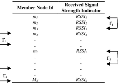
Figure 7.Figure 7. Segmentation architecture of member nodes inside a sector. Segmentation architecture of member nodes inside a sector. Table 2.Member table of a SH node.
J. Sens. Actuator Netw. 2016, 5, 2 10 of 21
Table 2. Member table of a SH node.
Member Node Id Received Signal Strength Indicator
m1 RSSI1
m2 RSSI2
m3 RSSI3
m4 RSSI4
.. ..
.. ..
mi RSSIi
.. ..
.. ..
.. ..
.. ..
MK RSSIk
3.5. Skyline Query
A threshold based hierarchical approach has been used in this research to calculate DS (q, r). The threshold based hierarchical approach uses the temporal correlation among the sectors and segments of a sector. All the key notations used in this section are listed in the Table 3 to increase reader comfort.
Table 3. Skyline Notation.
Symbol Description
ei An event at SHi or segment ri of a sector
E A set of events
θi The threshold point of SHi or Segment ri
LDSi The local dynamic skyline of SHi or Segment ri
𝑒𝑖≺(𝑞,𝑟) 𝑒𝑗 Event ej is dominated by event ei with respect to query point q and the target
region of interest is a circle of radius r centered at q.
𝑒𝑖≼(𝑞,𝑟) 𝑒𝑗 Event ej is dominated by or equal to event eiwith respect to query point q and
the target region of interest is a circle of radius r centered at q.
𝑒𝑖≺(𝑞,𝑟) 𝐸 Each event in Eis dominated by event ei with respect to query point q and the
target region of interest is a circle of radius r centered at q.
𝑒𝑖≼(𝑞,𝑟) 𝐸 Each event in Eis dominated by or equal to event eiwith respect to query
point q and the target region of interest is a circle of radius r centered at q.
Algorithm 3. Build_Tree(), implemented at each SH.
Input: n (total number of sectors (columns)), SELF_NET_ADDR
Output: Node (to store the node values), L (to store the address of left child of each node), R (to store
the address of right child of each node)
1: // Finding the Track (row) number of current sector
2: i = (SELF_NET_ADDR)/n;
3: index = S; 4: for j = 0 to S−1; 5: node [j] = (i, j) 6: if (i-1 ≥ 0)
7: L[j] = index;
8: N[index] = (i−1, j)
9: end if
10: Li= i−1
11: while (Li-1≥0)
12: L[index] = index + 1
13: Node[index] = (Li−1, j) 14: index++
15: Li--;
r
1r
2r
3r
43.5. Skyline Query
A threshold based hierarchical approach has been used in this research to calculateDS(q, r). The threshold based hierarchical approach uses the temporal correlation among the sectors and segments of a sector. All the key notations used in this section are listed in the Table3to increase reader comfort.
Table 3.Skyline Notation.
Symbol Description
ei An event atSHior segmentriof a sector
E A set of events
θi The threshold point ofSHior Segmentri LDSi The local dynamic skyline ofSHior Segmentri
eiăpq,rq ej Eventejis dominated by eventregion of interest is a circle of radiuseiwith respect to query pointrcentered atqqand the target.
eiďpq,rq ej Eventejthe target region of interest is a circle of radiusis dominated by or equal to eventeiwith respect to query pointrcentered atq. qand
eiăpq,rq E
Each event inEis dominated by eventeiwith respect to query pointqand the
target region of interest is a circle of radiusrcentered atq.
eiďpq,rq E
Each event inEis dominated by or equal to eventeiwith respect to query
Algorithm 3.Build_Tree(), implemented at each SH.
Input:n(total number of sectors (columns)),SELF_NET_ADDR
Output:Node(to store the node values),L(to store the address of left child of each node),R(to store the address of right child of each node)
1: // Finding the Track (row) number of current sector 2: i= (SELF_NET_ADDR)/n;
3: index=S; 4: forj= 0 toS´1; 5: node[j] = (i,j) 6: if(i-1ě0) 7: L[j] =index; 8: N[index] = (i´1,j) 9: end if
10: Li=i´1
11: while(Li-1ě0) 12: L[index] =index+ 1 13: Node[index] = (Li´1,j)
14: index++
15: Li–;
16: end while
17: index++ 18: if(i+1<T) 19: R[j] =index; 20: N[index] = (i+1,j) 21: end if
22: Ri=i+1
23: while(Ri+1<T) 24: R[index] =index+1 25: N[index] = (Ri+1,j)
26: index++
27: Ri++
28: end while
29: index++ 30: end for
3.5.1. Tree Structure Construction
J. Sens. Actuator Netw.2016,5, 2 12 of 22
16: end while
17: index++ 18: if (i+1<T) 19: R[j] = index;
20: N[index] = (i+1, j) 21: end if
22: Ri = i+1 23: while (Ri+1<T)
24: R[index] = index+1
25: N[index] = (Ri+1, j)
26: index++
27: Ri++ 28: end while
29: index++
30: end for
3.5.1. Tree Structure Construction
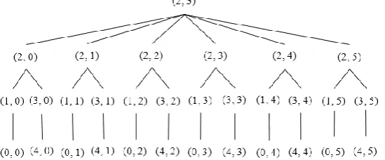
Each SH constructs a tree considering itself as the root using Algorithm 3. Figures 8 and 9 illustrate an example of the formation of a tree rooted at the 13th (2, 3) Sector. Sector (2, 0), (2, 1), (2, 2), (2, 3), (2, 4) and (2, 5) are the child nodes of Sector (2, 3). The sectors lying at the same column but upper row and lower row of each of the child nodes of root node are added to the left and right branch, respectively. For example, Sector (1, 0), (0, 0) and (3, 0), (4, 0) are added to the left and right branch, respectively, of Sector (2, 0). The hierarchy is further maintained among segments inside each sector, as shown in Figure 10.
Figure 8. SH of 13th Sector implies Algorithm 3 in order to convert the 5 × 5 grid into a tree rooted at
13th (2, 3) Sector.
Figure 9. Tree rooted at 13th Sector (2, 3).
Figure 8.SH of13thSector implies Algorithm 3 in order to convert the5ˆ5grid into a tree rooted at 13th(2, 3) Sector.
J. Sens. Actuator Netw. 2016, 5, 2 11 of 21
16: end while
17: index++ 18: if (i+1<T) 19: R[j] = index;
20: N[index] = (i+1, j) 21: end if
22: Ri = i+1
23: while (Ri+1<T)
24: R[index] = index+1 25: N[index] = (Ri+1, j)
26: index++ 27: Ri++
28: end while
29: index++
30: end for
3.5.1. Tree Structure Construction
Each SH constructs a tree considering itself as the root using Algorithm 3. Figures 8 and 9 illustrate an example of the formation of a tree rooted at the 13th (2, 3) Sector. Sector (2, 0), (2, 1), (2, 2), (2, 3), (2, 4) and (2, 5) are the child nodes of Sector (2, 3). The sectors lying at the same column but upper row and lower row of each of the child nodes of root node are added to the left and right branch, respectively. For example, Sector (1, 0), (0, 0) and (3, 0), (4, 0) are added to the left and right branch, respectively, of Sector (2, 0). The hierarchy is further maintained among segments inside each sector, as shown in Figure 10.
Figure 8. SH of 13th Sector implies Algorithm 3 in order to convert the 5 × 5 grid into a tree rooted at 13th (2, 3) Sector.
Figure 9. Tree rooted at 13th Sector (2, 3). Figure 9.Tree rooted at13thSector (2, 3).
J. Sens. Actuator Netw. 2016, 5, 2 12 of 21
Figure 10. Hierarchy based on segmentation.
3.5.2. Basic System Operation
A query node first calculates hash hq using Equation (10) for the Dynamic Skyline Query (DS (q, r)). The query is then forwarded to the SHi where Pi ≤ hq ≤ Pi+1. SHi finds the range of the query, i.e.,
[hq-r, hq+r]. Hence, the target sectors where the sample dataset of the query need to be considered are SHj, SHj+1,…, SHk, here Pj ≤ hq-r ≤ Pj+1, Pk ≤ hq+r ≤ Pk+1 and j ≤ k. The threshold based hierarchical approach
includes three phases—Tree Propagation, Regular Update and Triggered Query.
SHiissues a Triggered Query containing LSi to SHj+1, SHj+2 ..., SHk. The Triggered Query is issued to
ensure fetching all possible events that might be included in the final skyline but was not reported during the Regular Update phase. SHi sends Triggered Query to each of its child SHj that satisfies LSi θj. Any child node SHj satisfying LSi θjcan be discarded since no ineligible event can exist in the
final skytline. There cannot exist any event that can be eligible to be included in the final skyline. An
internal child node SHj after receiving Triggered QueryLSp from its parent computes LSj among LSp
and its non-reported points. SHj then forwards LSj to each of its children SHk that satisfies LSj θk
and waits for a reply with new points that are not dominated by LSj. SHjupdates the local skyline
after receiving replies from all of its child nodes and finally replies to its parent SHpwith the new
skyline event set. In contrast, a leaf node SHj reports nothing if it reports ej in the first phase or satisfies LSi θj. Otherwise, it reports event ej.
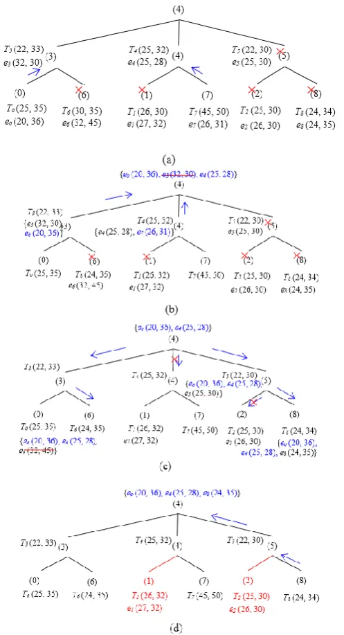
Figure 11 illustrates the functionality of the two phases—RegularUpdate and Triggered Query in a particular scenario. In the first phase (Regular Update) (Figure 11a), SH0 and SH7 reports eo and e7 to SH3 and SH4, respectively. However, e7 and e3 have been pruned by e4. Thus, the skyline set after the
first phase includes {e0, e4} (see Figure 11b). Figure 11c,d illustrates the second phase. SH4 issues a Triggered Query containing {e0, e4}to SH3, SH6, SH5, and SH8 (here, it is assumed that [hq−r, hq+r] covers
all the tree SH). SH0, SH1, SH7 and SH2, however, are discarded since their corresponding thresholds
are dominated by e4. After receiving the Triggered Query, SH5 prunes e5 and forwards the updated
skyline set {e0, e4} to SH8. SH8 calculates its local skyline and prunes among the query it receives from
its parent and its own event e8. Since e8 is not dominated, it has also been included into the final local
skyline set, i.e., {e0, e4, e8}, and is finally sent back to the SH4. It is to be noted that, during both phases, SH1 and SH2 do not need to transmit any event.
Figure 10.Hierarchy based on segmentation.
3.5.2. Basic System Operation
A query node first calculates hashhq using Equation (10) for theDynamic Skyline Query(DS (q, r)). The query is then forwarded to theSHiwherePiďhqďPi`1.SHifinds the range of the query, i.e., [hq-r,hq+r]. Hence, the target sectors where the sample dataset of the query need to be considered areSHj,SHj`1, . . . ,SHk, herePj ďhq´r ďPj`1,Pk ďhq`r ďPk`1andjďk. The threshold based hierarchical approach includes three phases—Tree Propagation,Regular UpdateandTriggered Query.
J. Sens. Actuator Netw.2016,5, 2 13 of 22
skyline event set. In contrast, a leaf nodeSHjreports nothing if it reportsejin the first phase or satisfies LSiĺθj. Otherwise, it reports eventej.
Figure11illustrates the functionality of the two phases—Regular UpdateandTriggered Queryin a particular scenario. In the first phase (Regular Update) (Figure11a),SH0andSH7reportseoande7 toSH3andSH4, respectively. However,e7ande3have been pruned bye4. Thus, the skyline set after the first phase includes {e0,e4} (see Figure11b). Figure11c,d illustrates the second phase.SH4issues aTriggered Querycontaining {e0,e4} toSH3,SH6,SH5, andSH8(here, it is assumed that [hq´r,hq+r] covers all the treeSH).SH0, SH1,SH7andSH2, however, are discarded since their corresponding thresholds are dominated bye4. After receiving theTriggered Query,SH5prunese5and forwards the updated skyline set {e0,e4} toSH8. SH8calculates its local skyline and prunes among the query it receives from its parent and its own evente8. Sincee8is not dominated, it has also been included into the final local skyline set,i.e., {e0,e4,e8}, and is finally sent back to theSH4. It is to be noted that, during both phases,SH1andSH2do not need to transmit any event.
Figure 10. Hierarchy based on segmentation.
3.5.2. Basic System Operation
A query node first calculates hash hq using Equation (10) for the Dynamic Skyline Query (DS (q, r)). The query is then forwarded to the SHi where Pi ≤ hq ≤ Pi+1. SHi finds the range of the query, i.e.,
[hq-r, hq+r]. Hence, the target sectors where the sample dataset of the query need to be considered are SHj, SHj+1,…, SHk, here Pj ≤ hq-r ≤ Pj+1, Pk ≤ hq+r ≤ Pk+1 and j ≤ k. The threshold based hierarchical approach
includes three phases—Tree Propagation, Regular Update and Triggered Query.
SHiissues a Triggered Query containing LSi to SHj+1, SHj+2 ..., SHk. The Triggered Query is issued to
ensure fetching all possible events that might be included in the final skyline but was not reported during the Regular Update phase. SHi sends Triggered Query to each of its child SHj that satisfies LSi θj. Any child node SHj satisfying LSi θjcan be discarded since no ineligible event can exist in the
final skytline. There cannot exist any event that can be eligible to be included in the final skyline. An
internal child node SHj after receiving Triggered QueryLSp from its parent computes LSj among LSp
and its non-reported points. SHj then forwards LSj to each of its children SHk that satisfies LSj θk
and waits for a reply with new points that are not dominated by LSj. SHjupdates the local skyline
after receiving replies from all of its child nodes and finally replies to its parent SHpwith the new
skyline event set. In contrast, a leaf node SHj reports nothing if it reports ej in the first phase or satisfies LSi θj. Otherwise, it reports event ej.
Figure 11 illustrates the functionality of the two phases—RegularUpdate and Triggered Query in a particular scenario. In the first phase (Regular Update) (Figure 11a), SH0 and SH7 reports eo and e7 to SH3 and SH4, respectively. However, e7 and e3 have been pruned by e4. Thus, the skyline set after the
first phase includes {e0, e4} (see Figure 11b). Figure 11c,d illustrates the second phase. SH4 issues a Triggered Query containing {e0, e4}to SH3, SH6, SH5, and SH8 (here, it is assumed that [hq−r, hq+r] covers
all the tree SH). SH0, SH1, SH7 and SH2, however, are discarded since their corresponding thresholds
are dominated by e4. After receiving the Triggered Query, SH5 prunes e5 and forwards the updated
skyline set {e0, e4} to SH8. SH8 calculates its local skyline and prunes among the query it receives from
its parent and its own event e8. Since e8 is not dominated, it has also been included into the final local
skyline set, i.e., {e0, e4, e8}, and is finally sent back to the SH4. It is to be noted that, during both phases, SH1 and SH2 do not need to transmit any event.
J. Sens. Actuator Netw. 2016, 5, 2 13 of 21
Figure 11. Basic Approach Example (3 × 3 Grids). (a) Regular update. (b) Skyline set after first phase. (c) Triggered query. (d) Skyline set after second phase
4. Performance Evaluation
Simulations were conducted using Castalia v3.2 [29] running on top of OMNET++ [31] to evaluate the performance of EDDS. The system parameters and their settings used in the experiments are summarized in Table 4. The network model (illustrated in Section 3.1) was tested in four rectangular fields with different parameter settings. Sensor MAC (SMAC) [32] and Sector Based Distance Routing (SBD) [15] are used in MAC and routing layer. Simulations were run 30~40 times with varying-channel affecting seeds to provide results that included average and 95% confidence interval. In Section 4.1, possible distribution of data throughout the network is presented. Section 4.2 evaluated EDDS in terms of energy consumption, latency and accuracy in a network of 180 nodes in a 90 m × 90 m (8100 m2) rectangular field. In Sections 4.3 and 4.4, the performance of EDDS was tested
using four different rectangular fields with four different distributions respectively. In Sections 4.5– 4.8, the performance of EDDS is evaluated against SkySensor in terms of data loss, data uniformity, success rate and resilience to node failure. In Section 4.9, customized EDDS is implemented on top of Q-NIGHT and evaluated against its performance in DBDCS.
4. Performance Evaluation
Simulations were conducted using Castalia v3.2 [29] running on top of OMNET++ [31] to evaluate the performance of EDDS. The system parameters and their settings used in the experiments are summarized in Table4. The network model (illustrated in Section3.1) was tested in four rectangular fields with different parameter settings. Sensor MAC (SMAC) [32] and Sector Based Distance Routing (SBD) [15] are used in MAC and routing layer. Simulations were run 30~40 times with varying-channel affecting seeds to provide results that included average and 95% confidence interval. In Section4.1, possible distribution of data throughout the network is presented. Section4.2evaluated EDDS in terms of energy consumption, latency and accuracy in a network of 180 nodes in a 90 mˆ90 m (8100 m2) rectangular field. In Section4.3, the performance of EDDS was tested using four different rectangular fields with four different distributions respectively. In Section4.4, the performance of EDDS is evaluated against SkySensor in terms of data loss, data uniformity, success rate and resilience to node failure.
4.1. Data Distribution
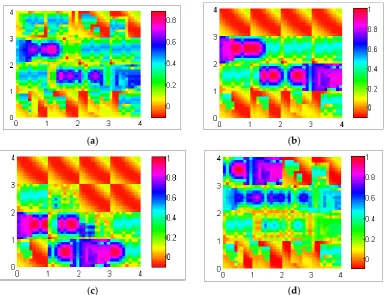
Figure12exploits different possible data dispersal with the realization of the mapping algorithm illustrated in Section3.2. This experiment was conducted in a network of 80 nodes in a 60 mˆ60 m (3600 m2, total number of sectors is 16 (4ˆ4)) field with a 60 min simulation time. The data production rate per sector was five packets per second. Figure12a shows uniform distribution, which means data are stored uniformly among all sectors of the network. Figure12b shows a central distribution in which data are usually located among central sector of the network. Figure12c,d represents the lower bound distribution and upper bound distribution, where data are stored among lower and upper sectors of the network, respectively.
J. Sens. Actuator Netw. 2016, 5, 2 14 of 21
4.1. Data Distribution
Figure 12 exploits different possible data dispersal with the realization of the mapping algorithm illustrated in Section 3.2. This experiment was conducted in a network of 80 nodes in a 60 m × 60 m (3600 m2, total number of sectors is 16 (4 × 4)) field with a 60 min simulation time. The data production
rate per sector was five packets per second. Figure 12a shows uniform distribution, which means data are stored uniformly among all sectors of the network. Figure 12b shows a central distribution in which data are usually located among central sector of the network. Figure 12c,d represents the lower bound distribution and upper bound distribution, where data are stored among lower and upper sectors of the network, respectively.
(a) (b)
(c) (d)
Figure 12. (a) Uniform distribution; (b) central distribution; (c) lower bound distribution; and (d) upper bound distribution.
4.2. Efficiency
The efficiency of the proposed approach is measured based on three parameters—energy consumption, latency and accuracy. These performance metrics and scalability of the proposed model is directly affected by the query range, which varies based on the average number of sectors indicated by α. With the increase of α, the number of messages that are generated due to three fundamental operations such as Tree Propagation, Regular Update and Triggered Query increases exponentially. Thus, in a model such as skyline query, it is an utmost challenge to minimize the energy consumption and latency while maximizing the accuracy. This experiment was conducted in a 90 m × 90 m rectangular field, in which 180 nodes were randomly and independently disseminated. The data distribution used in this experiment was uniform. The query rate varied from 0.1 to 0.5 queries per sector per second and the simulation was run for 60 min. The SkylineQuery overhead is comparatively high due to its three phase query calculation. Figure 13a–c presents the average energy consumption (J) per node, latency (s) and accuracy (accuracy was defined as the percentage of skyline queries that were correctly resolved) as a function of the query rate per sector per second. In this experiment, the query range was varied in four different ways as shown in Figure 13. In order to show the scalability of the system, α has been varied exponentially up to 36, where 36 is the total number of sectors in a 90 m × 90 m (Table 4) rectangular field. From Figure 13a,b, it is noted that the
4.2. Efficiency
The efficiency of the proposed approach is measured based on three parameters—energy consumption, latency and accuracy. These performance metrics and scalability of the proposed model is directly affected by the query range, which varies based on the average number of sectors indicated byα. With the increase ofα, the number of messages that are generated due to three fundamental operations such asTree Propagation,Regular UpdateandTriggered Queryincreases exponentially. Thus, in a model such as skyline query, it is an utmost challenge to minimize the energy consumption and latency while maximizing the accuracy. This experiment was conducted in a 90 mˆ90 m rectangular field, in which 180 nodes were randomly and independently disseminated. The data distribution used in this experiment was uniform. The query rate varied from 0.1 to 0.5 queries per sector per second and the simulation was run for 60 min. TheSkyline Queryoverhead is comparatively high due to its three phase query calculation. Figure13a–c presents the average energy consumption (J) per node, latency (s) and accuracy (accuracy was defined as the percentage of skyline queries that were correctly resolved) as a function of the query rate per sector per second. In this experiment, the query range was varied in four different ways as shown in Figure13. In order to show the scalability of the system,αhas been varied exponentially up to 36, where 36 is the total number of sectors in a 90 mˆ90 m (Table4) rectangular field. From Figure13a,b, it is noted that the overhead in terms of energy consumption and latency grows radically asαincreases. It is also to be noted that the data in Figure13a are presented in logarithmic scale in order to reduce the wide range to a more manageable size. However, the accuracy of the query response was very high (see Figure13c) and close to 100%. Packet loss due to interference causes some minor inaccuracy.
Table 4.Simulation Parameters.
Parameter Setting
Field Size (F) 60ˆ60 m2, 90ˆ90 m2, 120ˆ120 m2, 150ˆ150 m2 Number of Nodes (N) 80 (3600 m2), 180 (8100 m2), 320 (14,400 m2),
500 (22,500 m2)
Number of Sectors/Field Size (S/F) 16/(60ˆ60 m2), 36/(90ˆ90 m2), 64/(120ˆ120 m2), 100/(150ˆ150 m2)
Member Node Density (fm) 1 node/56.25 m2
Sector Head Node (SH) Density (fSH) 1 node/225 m2
Radio Range (member node) ~8 m
Radio Range (SH) ~20 m
Transmission Power 0 dBm (SH),´5 dBm (member node) Power Consumption in Sending and
Receiving Messages 57.42 mW (SH), 46.2 mW (member node)
Power Consumption Per Sensing 0.02 mJoule
Data Rate, Modulation Type, Bits Per Symbol, Bandwidth, Noise Bandwidth, Noise
Floor, Sensitivity
250 Kbps, PSK, 4, 20 MHz, 194 MHz,´100 dBm, ´95 dBm
pathLossExponent 2.4
Initial Average Path Loss (PL(d0)) 55
Reference Distance (d0) 1.0 m
Gaussian Zero-Mean Random Variable (Xα) 4.0
Routing Protocol SBD [15]
MAC Protocol, Maximum Transimission Retries SMAC [32], 2 SMAC Acknowledgment, Synchronization, RTS, CTS
J. Sens. Actuator Netw.2016,5, 2 16 of 22
overhead in terms of energy consumption and latency grows radically as α increases.It is also to be noted that the data in Figure 13a are presented in logarithmic scale in order to reduce the wide range to a more manageable size. However, the accuracy of the query response was very high (see Figure 13c) and close to 100%. Packet loss due to interference causes some minor inaccuracy.
Table 4. Simulation Parameters.
Parameter Setting
Field Size (F) 60 × 60 m2, 90 × 90 m2, 120 × 120 m2, 150 × 150 m2
Number of Nodes (N) 80 (3600 m
2), 180 (8100 m2), 320 (14,400 m2),
500 (22,500 m2)
Number of Sectors/Field Size (S/F) 16/(60 × 60 m2), 36/(90 × 90 m2), 64/(120 × 120 m2), 100/(150 × 150 m2)
Member Node Density (fm) 1 node/56.25 m2 Sector Head Node (SH) Density (fSH) 1 node/225 m2
Radio Range (member node) ~8 m
Radio Range (SH) ~20 m
Transmission Power 0 dBm (SH), −5 dBm (membernode) Power Consumption in Sending and
Receiving Messages 57.42 mW (SH), 46.2 mW (member node) Power Consumption Per Sensing 0.02 mJoule
Data Rate, Modulation Type, Bits Per Symbol, Bandwidth, Noise Bandwidth, Noise
Floor, Sensitivity
250 Kbps, PSK, 4, 20 MHz, 194 MHz, −100 dBm, −95 dBm
pathLossExponent 2.4
Initial Average Path Loss (PL(d0)) 55
Reference Distance (d0) 1.0 m
Gaussian Zero-Mean Random Variable (Xα) 4.0
Routing Protocol SBD [15]
MAC Protocol, Maximum Transimission
Retries SMAC [32], 2
SMAC Acknowledgment, Synchronization,
RTS, CTS Packet Size 11, 11, 13, 13 bytes
(a) (b)
J. Sens. Actuator Netw. 2016, 5, 2 16 of 21
(c)
Figure 13. (a) Energy consumption; (b) latency; and (c) accuracy.
4.3. Robustness
In this section, robustness of EDDS was evaluated through two different experiments with the variation of four different network sizes. In the first experiment, energy consumption, latency, and accuracy were measured for varying the query rate, while, in the second experiment, they were measured for four different data distributions.
4.3.1. Network Size
Experiments were carried out by varying the network field sizes such as 60 × 60 m2, 90 × 90 m2,
120 × 120 m2 and 150 × 150 m2 containing 80, 180, 320 and 500 nodes, respectively. The size of the
region of interest was kept fixed, i.e., the value of α was 9. The rate of the query was varied from 0.1 to 0.5 queries per sector per second. In Figure 14, the rate of the query is represented by β. Figure 14a,b demonstrates that energy consumption and latency is exponentially proportional to the value of β. However, when β is constant, they grow linearly with the size of the network. Figure 14c shows the percentage of accuracy as a function of network size. The accuracy drops slightly with the scale of the network.
(a) (b)
(c)
Figure 14. (a) Energy consumption; (b) latency; and (c) accuracy.
Figure 13.(a) Energy consumption; (b) latency; and (c) accuracy.
4.3. Robustness
In this section, robustness of EDDS was evaluated through two different experiments with the variation of four different network sizes. In the first experiment, energy consumption, latency, and accuracy were measured for varying the query rate, while, in the second experiment, they were measured for four different data distributions.
4.3.1. Network Size