Measuring Risk Structure Using the Capital Asset Pricing Model

227

Volume 63 29 Number 1, 2015

http://dx.doi.org/10.11118/actaun201563010227

MEASURING RISK STRUCTURE USING

THE CAPITAL ASSET PRICING MODEL

Zdeněk Konečný

_{, Marek Zinecker}

1 _{Department of Economics, Faculty of Business and Management, Brno University of Technology, Kolejní 2906/4,} 612 00 Brno, Czech Republic

Abstract

KONEČNÝ ZDENĚK, ZINECKER MAREK. 2015. Measuring Risk Structure Using the Capital Asset Pricing Model. Acta Universitatis Agriculturae et Silviculturae Mendelianae Brunensis, 63(1): 227–233. This article is aimed at proposing of an inovative method for calculating the shares of operational and fi nancial risks. This methodological tool will support managers while monitoring the risk structure. The method is based on the capital asset pricing model (CAPM) for calculation of equity cost, namely on determination of the beta coeffi cient, which is the only variable, that is dependent on entrepreneurial risk. There are combined both alternative approaches for calculation betas, which means, that there are accounting data used and there is distinguished unlevered beta and levered beta. The novelty of the proposed method is based on including of quantities for measuring operational and fi nancial risks in beta calculation. The volatility of cash fl ow, as a quantity for measuring of operational risk, is included in the unlevered beta. Return on equity based on the cash fl ow and the indebtedness are variables used in calculation of the levered beta. This modifi cation makes it possible to calculate the share of operational risk as the proportion of the unlevered/levered beta and the share of fi nancial risk, which is the remainder of levered beta. The modifi ed method is applied on companies from two sectors of the Czech economy. In the data set there are companies from one cyclical sector and from one neutral sector to fi nd out potential diff erences in the risk structure. The fi ndings show, that in both sectors the share of operational risk is over 50%, however, in the neutral sector is this more dominant. Keywords: beta coeffi cient, capital asset pricing model, fi nancial risk, operational risk, risk structure

INTRODUCTION

Every enterprise is connected with risks, which should be compensated by an equivalent return. The risk is usually measured as the rate of volatility of future cash fl ows and there are used statistical tools like standard deviation and coeffi cient of variation. But the return, required by investors, is expressed in the form of cost of capital, which is dependent on the rate of risk. So there is necessary to include the volatility of cash fl ow in the model of calculation cost of capital. There is evident, that the volatility of cash fl ow is typical especially for shareholders and other owners, whilst the future revenues of creditors are mostly guaranteed. And furthermore, the calculation of cost of debt is determined strictly, because the cost of debt are real payments, but the cost of equity is an implicit cost, because is it a required return, as mentioned above, and so there are more approaches of its calculation.

The most suitable and most used is the capital asset pricing model (CAPM), which consists of three variables. One of them, namely the beta coeffi cient, considers the entrepreneurial risk, which is either operational, or fi nancial. So there is a need for modifi cation the capital asset pricing model with an alternative estimation of the beta coeffi cient, which would estimate the operational and fi nancial risk separately.

Theoretical Background

Measuring Entrepreneurial Risks

The investment decisions are made either under certainty, or uncertainty. The decision making under uncertainty is much more frequent because of rapidly changing macroeconomic and microeconomic conditions. But in most cases, there is possible to quantify the uncertainty, because there are available future trends with their probabilities of occurrences. And this situation is called as decision making under risk. The term risk is defi ned as a quantifi ed uncertainty and its rate is determined by the probability of loss and by the hardness of potential impacts. But in the future, there can be reached either loss, or profi t, so there is necessary to distinguish a risk and an opportunity. The defi nition of both terms is mentioned by Vose (2008) as follows: • A risk is a random event, that may possibly occur and, if it did occur, would have a negative impact on the goals of the organisation. Thus, a risk is composed of three elements:

a) the scenario;

b) its probability of occurrence;

c) the size of its impact, if it did occur (either a fi xed value or a distribution).

• An opportunity is also a random event. That may possibly occur but, if it did occur, would have a positive impact on the goals of the organisation. Thus, an opportunity is composed of the same three elements as a risk.

There are many kinds of risks and many criteria of their classifi cation. For the purpose of measuring and managing risks is adequate to classify them according to the area of origin. So there are distinguished operational risks and fi nancial risks. A more described classifi cation of both kinds of risks is recorded in Reiners (2004) as follows:

1. Operational risks:

a) Risks having their origin in the entrepreneurial environment: economic risks, legal risks, currency risks, political risks, ecological risks, …

b) Business risks: sales risks, supplying risks, risks of entering new competitors (either direct competitors, or indirect competitors, that produce substitutes), …

c) Internal entrepreneurial risks: investment risks, production risks, risks of elektricity or IS/IT failure, personal risks, …

2. Financial risks:

a) Surety risks: legal form, ownership structures, guarantees, …

b) Risks of capital structure: risks of insolvency, risks of fi nancing, …

c) Risks of liquidity: direct and indirect risks connected with liquidity.

d) Risks of management: strategy of risk management, informational risks, …

There are more methods of measuring risk. Yan, Yu and Huang (2005) mention the approach by

Markowitz, who proposed measuring return and risk with mean and variance. Pfl ug and Ruszczyński (2005) give an explanation, that the mean refers to the average result among a set of possible scenarios, while the risk dimension describes the possible variation of the results under varying scenarios. So the rate of risk is measured by using the standard deviation as a square root of the variance, whose formula is mentioned e. g. in Jorion (2009):





 





n i i

x E X n

2

1

1 _{× ( ( ))}

1 .

Explanatory notes:

 ... standard deviation, n ... number of scenarios,

xi ... the values of the quantity, measured

i-times,

E (X) ... the average value of the measured quantity.

Besides the standard deviation, there is used also another statistical tool for measuring risk, namely the coeffi cient of variation, which is alternatively called as relative standard deviation or normalised standard deviation. Its calculation is the following:

 

CV

E X( ). Explanatory notes:

CV ... coeffi cient of variation,

 ... standard deviation,

E (X) ... the average value of the measured quantity.

The two basic advantages of the coeffi cient of correlation, compared to the standard deviation, can be found in Vose (2008):

1. The standard deviation is given as a fraction of its mean. Using this statistic allows the spread of the distribution of a variable with a large mean and correspondingly large standard deviation to be compared more appropriately with the spread of the distribution of another variable with a smaller mean and a correspondingly smaller standard deviation.

2. The standard deviation is now independent of its units. So, for example, the relative variability of the EUR:HKD and USD:GBP exchange rates can be compared.

Risks can be measured also by the indicator called Value at Risk (VaR), mentioned e. g. by Nielsson (2009). It can be defi ned as either the maximal loss of a fi nancial position under normal market conditions or the minimal loss under extraordinary market circumstances. Both defi nitions lead to the same Value at Risk, but the second one is more suitable for risk management.

which can be, according to this author, identifi ed with the strategic risk, because it is a risk of pursuing an ineff ective strategy. And for measuring business risk, there can be used three types of methods, as follows:

1. peers/analogue company approach; 2. statistical Methods;

3. scenarios.

And fi nally, some authors propose measuring instruments for both operational and fi nancial risks. According to Reiners (2004), whose classifi cation of risks was mentioned above, uses the volatility of cash fl ow for measuring operational risk and the rate of indebtedness for measuring fi nancial risk. An alternative approach can be found in Kislingerová (2001), who mentions, that the operational risk can be measured by the rate of operational leverage, which is calculated as the proportion of the year-on-year change of profi t in % to the year-year-on-year change of sales in %, and for measuring fi nancial risks can be used the proportion of the year-on-year change of profi t per share in % to the year-on-year change of earnings before interest and taxes (EBIT) in %, or the proportion of EBIT to the EBIT without cost interests. But there isn’t possible to calculate the shares of operational and fi nancial risks, because both models are characterized with a limitation, that for measuring operational risks are used diff erent quantities (in diff erent units) than for measuring fi nancial risks.

Capital Asset Pricing Model by Estimating Cost of Equity

The capital asset pricing model (CAPM) was developed by Sharpe (1964) and Lintner (1965) to calculate the expected returns of investors.

Furthermore, it can be applied also by estimating cost of equity, because the return of investors is the cost for the company.

This model is based on six basic and four additional simplifi ed assumptions, as mentioned by Sharpe, Alexander and Bailey (1999):

1. Investors evaluate portfolios by looking at the expected returns and standard deviations of the portfolios over a one-period horizon.

2. Investors are never satiated, so when given a choice between two portfolios with identical standard deviations, they will choose the one with the higher expected return.

3. Investors are risk-averse, so when given a choice between two portfolios with identical expected returns, they will choose the one with the lower standard deviation.

4. Individual assets are infi nitely divisible, meaning that an investor can buy a fraction of a share if he or she so desires.

5. There is a riskfree rate at which an investor may either lend (that is, invest) or borrow money. 6. Taxes and transaction costs are irrelevant. 7. All investors have the same one-period horizon. 8. The riskfree rate is the same for all investors. 9. Information is freely and instantly available to all

investors.

10. Investors have homogeneous expectations, meaning that they have the same perceptions in regard to the expected returns, standard deviations, and covariances of securities.

Nowadays, it is the most used model of calculation expected returns and cost of equity, as mentioned by Lee and Upneja (2008) or by Da, Guo and Jagannathan (2012). But through the history of

The Original CAPM

The Static CAPM

(single-period) The Dynamic CAPM (multi-period)

Existence of Equilibrium

Behavioral Finance

No Riskless Asset

Dividend and Taxation Effect Models

Equilibrium Models with Heterogeneity

Beliefs and Investors

Skewness Effect Models

Liquidity-based Models

Equilibrium Models with Heterogeneity

Investment Horizon

Intertemporal CAPM –

Merton Model

Supply -Side Effect Model

International CAPM

Intertemporal CAPM –

Consumption-based Models

Intertemporal CAPM – Production-based Models

using CAPM, there have been made some its modifi cations. On Fig. 1, there are depicted the most important models, based on CAPM, as mentioned by Shih, Chen, Lee and Chen (2013).

The basic formula for calculation cost of equity according to the capital asset pricing model is the following:

r = rf +  × (rm − rf). Explanatory notes:

r ... expected return of a stock within the portfolio (cost of equity),

rf ... riskfree rate,  ... beta coeffi cient,

rm ... expected market return,

(r_m − r_f) ... market risk premium.

So the cost of equity is determined by three variables. The only one factor, which is refl ective of the risk of the company, is the beta coeffi cient, which is quantifi ed using this formula:

 

  ₂im

m .

Explanatory notes:

 ... beta coeffi cient,

_im ... covariance with the market,

2

m... variance of the market.

According to Damodaran (2006), there are three methods, how to determine beta coeffi cient, which is derived from the characteristics of input data. 1. Historical market betas: this „classical“ approach

can be applied, if there are published historical data about market return and stock return. 2. Fundamental betas: this alternative approach is

applicable universally, it respects the basic three determinants of beta (type of business, degree of operating leverage, degree of fi nancial leverage) and there is distinguished unlevered beta, which is the beta coeffi cient of the company fi nanced only by equity, and levered beta, which is the unlevered beta adjusted on the indebtedness and the eff ective tax rate.

3. Accounting betas: if there aren’t published historical data about stock return, or if there isn´t a joint-stock company, there can be used accounting data about return on equity.

The purpose of this paper is to modify the alternative estimation of the beta coeffi cient to separate the premium on operational risks and the premium on fi nancial risks. This makes possible to distinguish the unlevered beta and levered beta mentioned by Damodaran (2006) and there will be applied the quantities for measuring operational and fi nancial risks recorded by Reiners (2004). A er this modifi cation, there will be possible to calculate the shares of operational and fi nancial risk and so to fi nd out the risk structure. This methodology will support more eff ective decision making of managers. They will receive a tool for more effi cient managing of operational and fi nancial risks. There

will be subsequently implemented a research on a sample of Czech companies, acting on two sectors with diff erent sensitivity to the economic cycle, measured by the coeffi cient of correlation between gross domestic product (GDP) and sales for own products, goods and services reached by the sector, which is identical to the market. So the sectors of the Czech economy will be classifi ed into cyclical, neutral and anti-cyclical sectors and the results will be compared with a similar research by Berman and Pfl eeger (1997) implemented in USA. On the basis of these two comparable researches, there will be selected one sector, which is typically cyclical and one sector, which is typically neutral. There will be selected no anti-cyclical sector, because there are very few anti-cyclical sectors and moreover, most characteristics of anti-cyclical sectors are analogous to cyclical sectors. A er that, there will be, across the companies from the both selected sectors, compared the shares of operational risks, determined by the proportion of unlevered beta to levered beta. So there is possible to fi nd out the share of fi nancial risks, too. The share of both operational and fi nancial risk can reach values just within the interval from 0 to 1, so it has a triangular distribution, called also as Simpson distribution, which is, besides the uniform and normal distribution, typical for fi nancial quantities, as mentioned by Brealey and Myers (2002) or by Brigham and Ehrhardt (2008). So there will be calculated, for both sectors, the basic characteristics of the triangular distribution, described in the methodical part.

MATERIAL AND METHODS

There will be combined an inductive and deductive approach, because there will be modifi ed the alternative method for calculation the beta coeffi cient and simultaneously, it will be applied in the quantitative research.

The data needed for determination the rate of sector sensitivity to the economic cycle and for estimation beta coeffi cient of selected companies are collected from the analytical materials published on the website by the Czech Statistical Offi ce (www.czso.cz) and the Czech Ministry of Industry and Trade (www.mpo.cz) and from the fi nancial statements of selected companies. The sample consists of companies limited by guarantee and joint-stock companies, regardless their size, operating on two sectors of the Czech economy with a diff erent sensitivity to the economic cycle.

   

  







=1

2 2

=1 =1

( ) ( )

( )

( ) ( )

n

i i i

i

n n

i i i

i i

sales sales GDP GDP

Correl sales,GDP

sales sales GDP GDP

.

Explanatory notes:

Correl(sales, GDP) ...coeffi cient of correlation between sales on the market and GDP,

salesi ...sales (for own products, goods and services) on the market, measured i-times,

sales ...average value of sales on the market,

GDPi ...GDP measured i-times, GDP ...average value of GDP,

n ...number of measuring sales on the market and GDP.

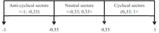
The coeffi cient of correlation can reach values from −1 to +1 and there is necessary to divide this interval into three partial intervals for cyclical, neutral and anti-cyclical sectors. To keep the identical probability of occurrence and thus to eliminate potential distortions, there is suitable to divide the interval into three thirds, as illustrated on Fig. 2.

A er selecting the neutral and cyclical sector, there will be selected a sample of companies from both these sectors. Subsequently, there will be collected the needed data from fi nancial statements and there will be calculated shares of operational and fi nancial risk using the modifi ed method of determination the beta coeffi cient. Then, there will be quantifi ed the basic characteristics of the triangular distribution for the share of operational risk, namely minimum, mode, maximum, probability density function for the value equal to mode, cumulative distribution function for the value equal to mode, mean, variance, skewness and kurtosis.

RESULTS

The modifi ed method of calculation the beta coeffi cient combines the two alternative approaches of estimation beta, mentioned by Damodaran (2006), namely fundamental betas and accounting betas. So there is distinguished the unlevered and levered beta and both these parts are calculated using accounting data, collected from fi nancial statements of selected companies. And there are respected

the instruments for measuring operational and fi nancial risk, suggested by Reiners (2004).

Calculation the Shares of Risks Using Unlevered and Levered Betas

As mentioned by Reiners (2004), operational risk can be measured by the volatility of cash fl ow. This measuring instrument can be included in calculation the unlevered beta, because there is possible to consider return on equity (ROE) based on cash fl ow instead of earnings a er taxes (EAT). So the formula for calculation unlevered beta, which is mentioned by Damodaran (2006), in order to quantify the rate of operational risk, can be modifi ed this way:



_{   }  _{   } 

  

__{ } _{ } _{ } _  _{ } _{ }

   

 



_{   }   _ _ _ _ 

 

 





=1

2

=1

t t

n

t m m c c

unlevered _t n

t m m

CF CF CF CF

E E E E

n CF CF

E E

n

.

Explanatory notes:

_unlevered ... beta of a company fi nanced only by equity,

CF ... cash fl ow, E ... equity,

 

 

 

t m CF

E .... return on equity of the market measured

t-times,

 

 

 m CF

E .... average return on equity of the market,

 

 

 

t c CF

E ... return on equity of the company

measured t-times,

 

 

 c CF

E ... average return on equity of the company,

n ... number of periods.

The fi nancial risk can be measured by the rate of indebtedness, as suggested by Reiners (2004). And according to Damodaran (2006), the levered beta is determined by adjusting the unlevered beta on the indebtedness (including the tax rate) as follows:

Anti-<

-1

-cyclical sec <-1; -0,33)

ctors

-0,33

Neutral se <-0,33; 0

ectors 0,33>

0

Cyclic (0,

,33

cal sectors ,33; 1>

1

2: Intervals of the coefficient of correlation for identification sectors with different sensitivity to the economic cycle





1 (1 ) 

levered unlevered

D t

E .

Explanatory notes:

levered ... beta of an indebted company,

_unlevered ... beta of the company fi nanced only by equity,

t ... eff ective tax rate, D ... debt,

E ... equity.

The levered beta includes both operational and fi nancial risk. So the second part of the previous formula, which is dependent on the tax rate and the indebtedness, is the rate of fi nancial risk. By the calculation levered beta, there is necessary to use the chronological average, recommended for time series, because there is changing the eff ective tax rate and also the shares of debt and ekvity from year to year.

Finding out Diff erences in Risk Structure Depending on the Sector Sensitivity There were selected two sectors of the czech economy, with respecting the classifi cation CZ-NACE. But by selecting the sample of companies, there was necessary to narrow the sector to minimize the diversity of companies. So there were selected two following sectors and samples of companies:

1. „Civil engineering“ as the cyclical sector – 9 of 57 companies from its partial sector „Construction of roads and railways“.

2. „Manufacture of chemicals and chemical products“ as the neutral sector – 8 of 44 companies from its partial sector „Manufacture of fertilisers and nitrogen compounds“.

As there was written above, the share of operational risk has a triangular distribution because of a limited set of reachable values. The basic statistical characteristics of this triangular distribution, including formulas of their calculation, for comparing shares of operational risk in the cyclical and neutral sector are recorded on Tab. I.

From the results, recorded on Tab. I can be derived, that in both sectors is the share of operational risk higher than one half and thus higher than the share of fi nancial risk. But by comparing the mode and mean values and also the cumulative distribution function and its skewness, there is evident, that in the neutral sector is the operational risk more dominant than in the cyclical sector.

So the entrepreneurship in the cyclical sector is more risky because of a high rate of volatility, but the shareholders are less sensitive to risks having their origin in enterprise itself. That means, that the riskiness is caused more signifi cantly by the risks connected with fi nancing the investments.

I: Comparing shares of operational risk in the cyclical and neutral sector using characteristics of the triangular distribution

Characteristics Additional description (symbol, formula, _{constant) the cyclical sector}Value for _{the neutral sector}Value for

Minimum a 0 0

Mode b 0.6 0.9

Maximum c 1 1

Probability density function

for mode  

2 ( )

( )

f x

c a 2 2

Cumulative distribution function for mode

 

 ( ) ( )

( )

b a F x

c a 0.6 0.9

Mean ( )(   )

3

a b c

E X 0.5333 0.6333

Variance      

2 2 2

( )

( )

18

a b c ab ac bc

D X 0.0422 0.0506

Skewness

 

   

 _{ }  _  _

 

 _  _ _  _

   

 _  

_{   } 

 

_{ } 

_{  } 

 

2

3

2 2

2 ( ) ₁ 2 ( ) _{1 9}

2 2

5

2 ( )

1 3

b a b a

c a c a

b a c a

−0.1913 −0.5448

Kurtosis 2.4 2.4 2.4

DISCUSSION AND CONCLUSION

Risk, as a quantifi ed uncertainty, must be measured to manage it. The most used method for measuring risk is using statistical tools like the standard deviation and the coeffi cient of variation. For measuring risk can be used also the quantity „Value at Risk“. But there are more kinds of risks, related to the entrepreneurial activities and so there is necessary to classify risks into groups and to measure each group of risks separately. The main aim of this article is to propose a new method for monitoring shares of individual kinds of risks and thus the risk structure. This method combines the alternative calculation of beta coeffi cient, which is a variable used in the capital asset pricing model, and quantities for measuring operational and fi nancial risk, proposed by Reiners (2004). The modifi cation of calculation unlevered beta is based on using cash fl ow, instead of earnings a er taxes, as an input variable and subsequently there is included the indebtedness and the eff ective tax rate and so there is calculated the levered beta. So the unlevered beta is identifi ed with the operational risk and the diff erence between levered and unlevered beta is equivalent to the part related to fi nancial risk. Similarly, the share of operational risk, which has a higher information ability, is calculated as the proportion of unlevered/levered beta. The contribution to the actual theory consists in calculating shares of operational and fi nancial risk and thus to fi nd out the risk structure. That indicates also its practical importance, because there is needed to know, which kind of risk dominates and so which kind of risk should managers focus on. The next aim of this article is to apply, and thus to verify, this method in the Czech entrepreneurial environment. So there are selected two sectors of the Czech economy, namely one cyclical and one neutral sector and there are calculated unlevered and levered betas by selected companies from both these sectors, using accounting data, collected from fi nancial statements. There are calculated characteristics of triangular distribution for the shares of operational risk to fi nd out diff erences between cyclical and neutral sector. And there was found out, that in the neutral sector is the share of operational risk considerably higher than in the cyclical sector.

Acknowledgement

This paper is supported by the Internal Grant Agency of the Brno University of Technology. Name of the Project: Economic Determinants of Competitiveness of Enterprises in Central and Eastern Europe. Project Registration No. FP-S-15-2825.

REFERENCES

BERMAN, J. and PFLEEGER, J. 1997. Which industries are sensitive to business cycles? Monthly Labor Review, 2: 19–25.

BREALEY, R. A. and MYERS, S. C. 2002. Financial Analysis with Excel.

BRIGHAM, E. F. and EHRHARDT, M. C. 2008. Financial Management. Theory and Practice. 12th _{Edition. Mason: Thomson South-Western.}

DA, Z., GUO, R. and JAGANNATHAN, R. 2012. CAPM for estimating the cost of equity capital: Interpreting the empirical evidence. Journal of Financial Economics, 103: 204–220.

DAMODARAN, A. 2006. Damodaran on Valuation: Analysis for Investment and Corporate Finance. 2nd _{Edition. New York: John Wiley & Sons.}

DOFF, R. 2008. Defi ning and measuring business risk in an economic-capital framework. The Journal of Risk Finance, 9(4): 317–333.

JORION, P. 2009. Financial Risk Manager Handbook. 5nd _{Edition. New Jersey: John Wiley & Sons.}

KISLINGEROVÁ, E. 2001. Oceňování podniku. 2nd _{Edition. Praha: C. H. Beck.}

LEE, S. and UPNEJA, A. 2008. Is Capital Asset Pricing Model (CAPM) the best way to estimate cost-of-equity for the lodging industry? International Journal of Contemporary Hospitality Management, 20(2): 172– 185.

LINTNER, J. 1965. The Valuation of Risk Assets and the Selection of Risky Investments in Stock Portfolios and Capital Budgets. The Review of Economics and Statistics, 47(1): 13–37.

NIELSSON, U. 2009. Measuring and regulating extreme risk. Journal of Financial Regulation and Compliance, 17(2): 156–171.

PFLUG, G. Ch. and RUSZCZYŃSKI, A. 2005. Measuring Risk for Income Streams. Computational Optimization and Applications, 32: 161–178.

REINERS, M. 2004. Finanzierungskosten im Lebenszyklus der Unternehmung. Ein optionspreistheoretischer Ansatz. Hamburg: Verlag Dr. Kovač.

SHARPE, W. F. 1964. Capital Asset Prices: A Theory of Market Equilibrium under Conditions of Risk. The Journal of Finance, 19(3): 425–442.

SHARPE, W. F., ALEXANDER, G. J. and BAILEY, J. V. 1999. Investments. 6th _{Edition. New Jersey: Prentice}

Hall.

SHIH, Y., CHEN, S., LEE, C. and CHEN, P. 2013. The evolution of capital asset pricing models.

VOSE, D. 2008. Risk Analysis. A Quantitative Guide. 3rd _{Edition. Chichester: John Wiley & Sons.}

YAN, C., YU, P. and HUANG, Y. 2005. Calculation of Expected Shortfall for Measuring Risk and Its Applications. Journal of Shanghai University, 9(1): 90– 94.

Contact information Zdeněk Konečný: [email protected]