Emperor International Journal of Finance and Management Research [EIJFMR] Page 155
TESTING THE EFFECTIVENESS OF A
TECHNICAL ANALYSIS STRATEGY
VERSUS BUY-AND-HOLD STRATEGY IN
INDIA CASE STUDY OF SENSEX
(BSE 30)
ARUNANGSHU DAS SARMA Lecturer
Lalbaba College, 117, G.T. Road, Post Belurmath, Howrah, West Bengal 711201
Shibpur Dinobundhoo Institution (College), 412/1, G.T. Road (South), Shibpur, Howrah, West Bengal 711102
Abstract
Efficient market hypothesis (EMH) and the random
walk theory are the two central concepts that explains the
financial market efficiencies. According to the EMH and
random walk theory, if a market is efficient, it is not
possible to it is not possible to forecast future share prices
with the use of historical stock prices. The profitability of
technical trading has been extensively debated previously,
but as yet there is no consensus among the economists.
Therefore this gives an impetus to continue the study. I
have done it by applying the moving average
convergence/divergence (MACD) technical indicator, to
roughly the last 10 years historical prices of the Bombay
Stock Exchange index, and tried to find out whether it can
beat the normal market returns or not. And thereby having
an idea as to which strategy should be followed by the
investors.
I. INTRODUCTION
Fundamental analysis is a share trading strategy that tries to calculate the intrinsic value of a particular stock with the help of financial data’s like revenue, expenditure growth prospects of the company and its competitive environment. There are many fundamental factors that an analyst needs to study for the analysis of the stock. Some of them are, the company’s basic information, the financial statements of the company, the micro and macro-economic factors, the industry to which the company belongs, and the company’s future plans. And depending on
the comparison between the intrinsic value and market value the analyst then will make a “BUY”, “SELL” or “HOLD” recommendation.
“BUY-AND-HOLD” strategy is closely related to fundamental analysis. Buy-and-Hold strategy is and investment strategy in which the investor buys a stock and holds it for a long period of time as he believes that despite the short-term volatility in the stock market, the long term returns on the stock can be reasonable. Investors tries to find stocks with low relative valuation as their starting point, by using price multiples such as EV/Sales, P/E, EV/EBIDTA, P/B. They Buy-and-Hold these stocks in the apprehension that in the long run the prices will adjust and reflect their intrinsic value. The Buy-and-Hold strategy also means lower expense in terms of transaction cost, and the ability to receive future dividends. A Buy-and-Hold strategy is therefore considered as a long-term investment strategy as there are few transactions taking place.
Emperor International Journal of Finance and Management Research [EIJFMR] Page 156 analysis used stock information like, price, volume,
open interest on a chart and applies various patterns and indicators to it, to assess the future price movements. Many buy and sell signals get generated in different scenarios. Therefore an investment strategy following technical analysis can be termed as a short-term strategy as in this strategy many buy and sell signals gets generated. However, technical analysis is criticized as it involves huge amount of transaction cost, which in turn offsets the return earned through this strategy, to some extent.
Some of the popular indicators can be given as, Moving Average (MA), Moving Average Convergence/Divergence (MACD), Relative Strength Index (RSI), Average True Range (ATR), Stochastic Oscillators etc. among other technical trading indicators. Moving average rules, trading range break-out rules and filter rules are given by Lakonishok & LeBaron (1992), Levich & Thomas (1993), Sullivan, Timmermann, & White (1999), Griffioen (2003), as having the predictability of future prices.
Moving Average Convergence/Divergence (MACD), developed by Gerald Appel in 1979, in one of the most simplest and reliable indicator in technical analysis. An advantage of MACD over other technical indicators is that it incorporates both momentum and trend-following characteristics in one indicator. As a trend-following indicator, MACD follows the trend of the underlying stock since it is constructed from two exponential moving averages of the closing price. As a momentum indicator MACD indicates the whether the trend in price is gaining strength or losing momentum, this can be followed as the MACD line oscillates above and below the center zero line. Therefore MACD is used in predicting the changes in stock trend and potential reversal points of the stock.
Objectives
The study aims at investigation of whether the
technical indicator (MACD) produced better return in comparison to the Buy-and-Hold strategy in the period from 2nd January, 2007 to 18th January, 2017. In other words, this research paper tries to find out as to which trading strategy is more effective – a strategy with few transactions versus a strategy with constant buying and selling.
The research hypothesis can be given as:
The null hypothesis is that the means returns from both the strategies are equal, and the alternative hypothesis being that the mean returns are not equal.
In short it can be said:
H0: Buy-and-Hold return = MACD return H1: Buy-and-Hold return ≠ MACD return A significant level of 5% has been applied in this test.
The hypothesis for correlation is given by: H0 = The returns from the Buy-and-Hold strategy and the MACD strategy are not significantly correlated.
H1 = The returns from the Buy-and-Hold strategy and the MACD strategy are significantly correlated.
II. LITERATURE REVIEW
Pistole &Metghalci have used historical data of S&P 500 and have back tested it with SMA and PSAR to show results of comparison between mechanical system of trading and the buy and hold strategy. While the SMA could not give better significance, so to conclude that it can beat the buy and hold strategy, results of PSAR method were statistically significant at the 95% level. So clearly PSAR method could beat the market to earn better returns. The results were same over both longer and shorter period.
Emperor International Journal of Finance and Management Research [EIJFMR] Page 157 trading didn’t generate any above normal gain as
opposed to the gains generated by the buy and hold strategy.
Sweeney (1988), Brock, Lakonishok and LeBaron (1992) tested the stock prices with the moving averages and the trading range breaks. One must keep in mind that brokerage firms always shows some buy and sell signals to get transactions as this is their source of revenue, so data’s from brokerage houses may not be reliable. They used data of Dow Jones Index from 1897 to 1986. They supported the use of technical analysis. According to them, technical trading gave more return as compared to the buy and hold strategy.
Bessembinder & Chan (1998) supported the Brock et al analysis, and confirmed their basic findings. But observed that the opportunity to trade, using technical indicators can coexist with market efficiency. He also said that, the basic results holds good but, the consideration of transaction cost and will certainly diminish the returns from the technical trading.
Gunasekaragea and Power (2001) use the moving average method to examine its effect in the Asian markets and concluded in favour of technical analysis, and that these were not in weak form of market efficiency.
Research Methodology
Research approach and software’s applied
In this paper an attempt has been made to calculate the predictability of technical analysis, with the help of a technical indicator – Moving Average Convergence/Divergence (MACD). This is done taking the daily open, high, low, close price of the BSE index from 2/1/12007 to 18/1/2017. Therefore all the data’s are historical in nature. The data is collected from yahoo finance database. The data collected has been analyzed using Microsoft Excel, which has been used to compute MACD, signal values, returns from the transactions and “Buy” and
“Sell” signals. It has also been used to generate charts. The other software that has been used is the IBM SPSS Statistic version 20. This has been used to prepare the charts, to do the correlation, regression analysis and to find the t-statistic.
Research Design
Assumptions that has been made in the study. The following assumptions has been made for the purpose of the study and the characteristics of the BSE SENSEX
1. The transaction price (both for buying and selling) for the index has been taken as the closing price of the day.
2. It is assumed that the amount available at the beginning is sufficient for the transaction. And it is also assumed that there are enough stocks to be bought.
3. The settlement date has been taken as T+0, that is investors get their stock or cash, when they buy or sell stock, on the day of the transaction itself. This is far from reality though.
4. Investors are able to buy or sell odd number of units.
5. The option of short selling has not been considered.
Study Method
A fair bit of work of this paper depends on Microsoft Excel. The following steps has been done in excel.
Step 1. Calculation of EMA, MACD and signal (9-day EMA of MACD)
EMA (current day) = price (current day) *(2/ (T+1)) + EMA (previous day) (1-(2/T+1))
Where:
Price (current day): closing price of the current day
T: time period (like: EMA (26) means T = 26) 2/ (T+1): the exponential percentage
Emperor International Journal of Finance and Management Research [EIJFMR] Page 158 T = (2/ exponential percentage) – 1
MACD Calculation
To calculate the MACD we need to subtract the value of the 26-day exponential moving average from the 12-day exponential moving average.
MACD = EMA (12) – EMA (26)
The 9-day exponential moving average is calculated on the MACD, which works as the signal line. Then it is plotted on the top of MACD
Signal line = EMA (9-day MACD)\
Step 2. Generating “Buy” and “Sell” signals as a basic trading method of MACD. When the MACD > Signal then “Buy” signal would be generated, and if MACD < Signal then “Sell” signal would be produced.
Step 3. Then the returns of the two strategies, namely MACD and Buy-and-Hold strategy.
It is calculated in the following manner:
Return = (Ending value – Beginning value) / Beginning value
Step 5. Then correlation, regression and a paired t-statistic to determine if there is any difference in the mean return from the two strategies, is performed with the help of IBM SPSS version 20. Correlation is computed between the returns from the buy-and-hold
strategy and the returns from the MACD strategy. Theoretical Discussion
Theories related to Technical Analysis.
Moving Average Convergence/Divergence Indicator (MACD)
Introduction
Moving average convergence/divergence indicator (MACD) is a trend following momentum indicator which shows relationship between two moving averages of a stock price. It was developed by Gerald Appel, the publisher of “Systems and Forecasts” in 1979. MACD is calculated by subtracting a 26-day moving average of the stock price from a 12-day moving average of the price of the same stock. The resulting indicator oscillate above and below the central zero line.
When the MACD indicator is above the Zero line, it means that the 12-day moving average is higher than the 26-day moving average. This is a bullish sign, as it shows that the current expectations (i.e., the 12-day moving average) are more optimistic than the previous expectations (i.e., the 26-day moving average). When MACD falls below the central zero line, it means that the 12-day moving average is less than the 26-day moving average.
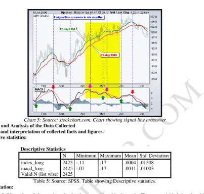
Emperor International Journal of Finance and Management Research [EIJFMR] Page 159 In the above example, the area shaded yellow shows the moving average convergence/divergence (MACD) line in negative area as the 12-day exponential moving average (EMA) is trading below the 26-day exponential moving average (EMA). The initial cross occurred at the end of September (indicated by the black arrow) and the MACD moved further into negative territory as the 12-day exponential moving average (EMA) diverged further from the 26-day exponential moving average (EMA). The area shaded orange highlights a period of positive moving average convergence/divergence (MACD) values that is when the 12-day exponential moving average (EMA) was above the 26-day exponential moving average (EMA). One should take note that the moving average convergence/divergence (MACD) line can be seen below 1 during this period of time (represented by the red dotted line). This means the distance between the 12-day exponential moving average (EMA) and 26-day exponential moving average (EMA) was less than 1 point, which is not a big difference. A 9-day moving average of the moving average convergence/divergence (MACD) line (not of the stock price) is generally plotted with the MACD indicator as a signal line. The signal line tries to anticipate the convergence of the two moving averages (i.e., movement of the MACD towards the central zero line).
Chart 2: Source: stockcharts.com. chart showing the MACD and Signal line. In the figure above the signal line is shown in the red line, and the MACD is line is shown in black. Uses of MACD
MACD can be traded in three ways: overbought/oversold conditions, divergences and crossovers. Overbought and oversold conditions.
Emperor International Journal of Finance and Management Research [EIJFMR] Page 160 Chart 3: Source: psgonline.co.za. Chart showing the overbought/sold areas of MACD
Divergence
Sometimes it so happens that the security price is trending in one direction, which should get confirmed by the indicator, but instead the indicator is seen trending in the opposite direction. That is when the divergence occurs, which tells that there is a trend reversal in the offing.
Chart 4: Source: stockchart.com. Chart showing divergence of MACD. The chart above shows the divergence in the price trend and the indicator.
Crossover
This is one of the most basic trading rule of the MACD indicator. A “BUY” signal appears when the MACD rises above the signal line. Similarly, a “SELL” signal appears when the MACD drops below the signal line.
Emperor International Journal of Finance and Management Research [EIJFMR] Page 161 Chart 5: Source: stockchart.com. Chart showing signal line crossover
Findings and Analysis of the Data Collected
Analysis and interpretation of collected facts and figures. Descriptive statistics:
Descriptive Statistics
N Minimum Maximum Mean Std. Deviation
index_long 2425 -.11 .17 .0004 .01508
macd_long 2425 -.07 .17 .0011 .01003
Valid N (list wise) 2425
Table 5: Source: SPSS. Table showing Descriptive statistics. Interpretation:
There are 2425 number of observations that has been considered in the study. The two variable being the, daily return from the Buy-and-Hold strategy (index_long) and the daily return from the MACD strategy.
The minimum and the maximum return from the Buy-and-Hold strategy over the period (21/03/2007 to 18/01/2017), has been negative eleven percent (11%) and seventeen percent positive (17%) respectively. And that from the MACD strategy has been negative seven percent (7%) and seventeen percent positive (17%). Therefore the range or the variability of the Buy-and-Hold strategy was more than the MACD strategy during the period.
The average daily return of the Buy-and-Hold strategy was 0.04% from (21/03/2007 to 18/01/2017) and from the MACD strategy the average daily return was 0.11% (21/03/2007 to 18/01/2017).
Therefore on a daily basis MACD gave more return as compared to the Buy-and-Hold strategy by 0.07% (0.11% - 0.04%)
The standard deviation of the Buy-and-Hold strategy was 0.01508 during the period, which means that on an average the returns were 0.01508 units away from the mean return. Similarly, the mean deviation of the returns of the MACD strategy was 0.01003 units from its mean return.
As it has been observed that the returns from Buy-and-Hold strategy was more scattered as compared to the MACD strategy.
Paired T-test
The hypothesis is given by:
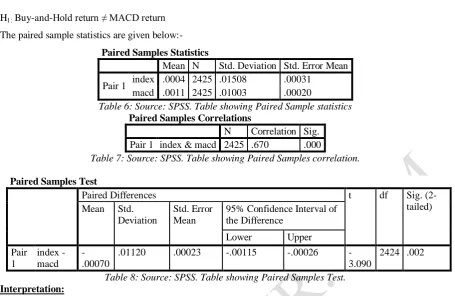
Emperor International Journal of Finance and Management Research [EIJFMR] Page 162 H1: Buy-and-Hold return ≠ MACD return
The paired sample statistics are given below:- Paired Samples Statistics
Mean N Std. Deviation Std. Error Mean Pair 1 index .0004 2425 .01508 .00031
macd .0011 2425 .01003 .00020
Table 6: Source: SPSS. Table showing Paired Sample statistics Paired Samples Correlations
N Correlation Sig. Pair 1 index & macd 2425 .670 .000
Table 7: Source: SPSS. Table showing Paired Samples correlation.
Paired Samples Test
Paired Differences t df Sig.
(2-tailed) Mean Std.
Deviation
Std. Error Mean
95% Confidence Interval of the Difference
Lower Upper
Pair 1
index - macd
-.00070
.01120 .00023 -.00115 -.00026
-3.090
2424 .002 Table 8: Source: SPSS. Table showing Paired Samples Test.
Interpretation:
As it can be seen that p-value = 0.002 < 0.05. Therefore the null hypothesis of equal means gets rejected, and the alternative hypothesis gets accepted. Differently put, the mean return from the Buy-and-Hold strategy is significantly different from the mean return from the MACD strategy, at the 5% level of confidence.
Test of correlation:
Correlation is a statistical measure that shows, to what an extent two variables fluctuate together. It measures the strength of association between the two variables.
The hypothesis is given by:
H0 = The returns from the Buy-and-Hold strategy and the MACD strategy are not significantly correlated.
H1 = The returns from the Buy-and-Hold strategy and the MACD strategy are significantly correlated.
Correlations
index_long macd_long index_long
Pearson Correlation 1 .670**
Sig. (2-tailed) .000
N 2425 2425
macd_long
Pearson Correlation .670** 1 Sig. (2-tailed) .000
N 2425 2425
**. Correlation is significant at the 0.01 level (2-tailed). Table 9: Source: SPSS. Table showing Correlations.
Interpretation:
Emperor International Journal of Finance and Management Research [EIJFMR] Page 163 Regression Analysis
Variables Entered/Removeda Mod
el
Variables Entered
Variables Removed
Method
1 index_longb . Enter
a. Dependent Variable: macd_long b. All requested variables entered. Table 10: Source: SPSS. Table showing Variables
Entered/Removed.
This table shows the independent variable entered as the independent variable and the dependent variable. Here the independent variable is the index_long, and the dependent variable is the macd_long.
Model Summery
The model summary table checks the goodness of the model. The coefficient of determination R2 is a summary measure that tells us how well the sample regression line fits the data. The value of R2 ranges between 0 and 1. More closely the value of R2 to 1, more comprehensively the independent variables explain the dependent variable.
Model Summary
Model R R Square Adjusted R Square Std. Error of the Estimate
1 .670a .449 .449 .00744
a. Predictors: (Constant), index_long
Table 11: Source: SPSS. Table showing Model Summery.
The value of R square is 0.449. It means that 44.9% of the variation in the dependent variable (i.e. MACD_long) can be explained by the selected independent variables (i.e. index_long) and 51.1% of the variation in the dependent variable remains unexplained. Thus, the model has moderate goodness of fit.
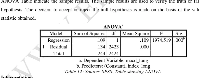
Anova Table
ANOVA Table indicate the sample results. The sample results are used to verify the truth or falsity of a null hypothesis. The decision to accept or reject the null hypothesis is made on the basis of the value of the test statistic obtained.
ANOVAa
Model Sum of Squares df Mean Square F Sig. 1
Regression .109 1 .109 1974.519 .000b
Residual .134 2423 .000
Total .244 2424
a. Dependent Variable: macd_long b. Predictors: (Constant), index_long Table 12: Source: SPSS. Table showing ANOVA. Interpretation:
From the above table the P-value is less than 0.05 indicating the probability that the calculated value of F-statistics is as much as or greater than what is obtained and falls in critical region i.e., less than 5%. This again confirms that the model can be accepted.
Coefficient
Emperor International Journal of Finance and Management Research [EIJFMR] Page 164 Coefficientsa
Model Unstandardized Coefficients Standardized Coefficients t Sig.
B Std. Error Beta
1 (Constant) .001 .000 6.213 .000
index_long .445 .010 .670 44.436 .000
a. Dependent Variable: macd_long
Table 13: Source: SPSS. Table showing the coefficients. The general estimated equation can be given by:
Y= β1X1 + β2X2 + β3X3 + constant
Therefore the equation would be:
MACD = 0.445index_long (p = 0.000) + 0.001(p = 0.000)
Here the “index_long” is statistically significant at the 5% level of confidence.
Therefore, higher is the return from the index, higher is the return from MACD. For every 1 rupee rise in the return of index there is a 0.445 rupee rise in the return of MACD. The returns from the two strategies shows a moderate positive relation.
Chart 7: Source: self-generated. Chart showing the regression line in EXCEL
The chart shows the regression line along with the points and regression equation, as created is Microsoft Excel.
Emperor International Journal of Finance and Management Research [EIJFMR] Page 165 III. CONCLUSION
In fundamental analysis an investor tries to estimate the market value of a stock by estimating future cash flows and the cost of capital. According to the EMH, all information (from fundamental analysis) should be reflected in the current price. An investor relying on technical analysis will argue that prices reflects current information, but stock prices will move in patterns due to concepts such as human biases, noise trading and the self-fulfilling prophecy element of technical analysis. These patterns can be predicted by chart analysis and calculations of different indicators
To conclude, the technical trading strategy based on MACD has been back-tested to show the results when compared with the traditional Buy-and-Hold strategy. Clearly as it can be seen that for the last ten years (from 2007 to 2017) trading with technical indicators has been able to provide us with more than normal returns. So statistically the results from the Moving Average Convergence/Divergence method do generate confidence greater than 95% confidence level, which has not been found in case of the traditional strategy. These findings are seen to be true over the last ten year period.
Therefore according to the study, as technical trading generates more than normal returns, it can be the strategy to be followed.
However, improvements in the method of computation of returns from both the strategies could have been made better. Transaction cost and positions on, before or after “Big Days” has not been considered separately, which could have given a significantly different result (i.e. return from technical strategy would have dipped). Yet on the other hand had I used stop loss, return from technical strategy could have been way higher, and yet again using stop loss on a historical data, and in real day to day life will not fetch the same result with the same
efficiency. Although, none of the strategies are infallible.
IV. SCOPE OF FURTHER STUDY
As has been said earlier, that transaction costs and positions on, before or after “Big Days”, have not been considered, a further study can be made taking these into consideration. A need to consider several technical trading strategies is also felt. Moreover a study considering both longer and shorter period is also needed.
V. REFERENCE
1) Achelis, S. B. (2000). Technical Analysis from A to Z. McGraw-Hill.
2) Becker, L. A., & Seshadri, M. (2003). GP-evolved technical trading rules can outperform Buy and Hold. Sixth International Conference on Computational Intelligence and Natural Computing. North Carolina, USA.
3) Bonga, W. G. (2015). The Need for Efficient Investment: Fundamental Analysis and Technical Analysis. Social Science Research Network (SSRN).
4) Brock, W., Lakonishok, J., & LeBaron, B. (1992). Simple Technical Trading Rules and the Stochastic Properties of Stock Returns. Journal of Finance, 1731-1764.