ESTIMATION OF OPTIMAL PATH ON URBAN ROAD NETWORKS
USING AHP ALGORITHM
Surendra Kukadapwar1, Dhananjay Parbat2
1, 2 Department of Civil Engineering, Government Polytechnic, Nagpur, India
Received 14 September 2015; accepted 29 January 2016
Abstract: This paper describes to develop a multi criteria decision based methodology to find optimal path in real urban road network. Over the year several studies were conducted but most of which rely on single variable like travel distance or travel time as cost function. In this study, seven different attributes influencing the traffic network i.e. distance, time, traffic volume, road width, no. of intersection, parking and encroachment on road are used to define cost function using multi criterion decision making approach. These variables are combined using a Multi-Dimensional Cost Model (MDCM) using the Analytical Hierarchical Process (AHP). The models developed were implemented and closely evaluated in Nagpur city of India. Model is considered for determining optimal path between various Origins and Destinations in real urban traffic network. Composite weighted AHP scored were used to generate AHP decision surface. Finally, the best decision was proposed by generating the least cost path which is considered as optimal path. The resulting routes showed to be more accurate than those obtained utilizing one-dimensional cost functions and AHP is found to be effective tool to deal with optimal route selection problem.
Keywords:optimal path, AHP, MADM, traffic congestion.
1 Corresponding author: [email protected]
1. Introduction
Due to rapid urbanization, the tremendous rise in number of vehicles is variably accompanied by ever increasing volume of traffic and intense traffic congestion on roads. Almost every city in India is facing acute traffic problem in regards to delay, congestion, pollution, accidents, parking etc. These problems contribute not only loss of precious manpower but also results in additional fuel consumption, development of mental stress and overall feel bad environment for the driver. Since traffic congestion has been one of the major issues that most of the metropolises are facing, the important task for researcher is to
find corrective measure and one of it may be to find shortest path between origin & destination sources which is not only optimal distant but carry minimum costs for other criterion such as travel time, traffic volume, no. of road junctions, roadside parking, encroachment’s along the road etc.
a time-dependent transportation network is a challenging task. This article proposes the spatial analysis of finding the optimal path between any two specific locations in a road network of the city where traffic condition changes continuously with time.
The route guidance system provides an optimum route to drivers based on a cost function and a route solution. The cost function is related to the distance towards destination, travel time (TT), or the cost of a road segment, etc. The route choice mechanism can provide the optimum route for drivers, based on the cost function. The route selection mechanism is the key technique of vehicle navigation systems providing route-planning strategy for travelers. Defining suitable mathematical models to represent the route selection mechanism in traditional methods uses numerical techniques and methods where perceived traffic attributes are treated as crisp inputs. However, much of human reasoning is based on vague, imprecise, and subjective values. Thus, the traditional methods ignore the presence of vagueness and ambiguity in drivers’ perception, making them difficult to be valid mathematical models. Traffic attributes as distance, travel time, traffic volume, encroachment and parking on road, road width and number of intersections were considered for problem of study.
The research paper is organized as follows, Section 2 describes the state of art literature, Section 3 describes the brief overview of M A DM method like A HP, Section 4 describes the experimental setup and scenario considered for study, followed by weight estimation AHP and various experimental analysis for different criteria’s like shortest path over specified origin &
destination zone using individual attributes and optimal path over specified origin & destination zone using MADM methods. Last the conclusion and outlook towards future research work is presented in Section 5.
2. Literature Review
Efficient management of traffic network requires, the shortest route from one point (node) to another is known; this is termed as the shortest path. “Optimal” refers to shortest time, shortest distance, or least total cost. Finding the shortest path is an important task in any network and transportation related analyses. This problem arises as a main decision question or as a step in some situation. There are many variations, depending on the type of network and costs involved, and source/ destination pairs of nodes for which we need solution (Rardin, 2003). As per shortest path algorithm by Dijkstra (1959), each node is labeled with its distance from the source node along the best-known path. Initially, no paths are known, so all nodes are labeled with infinity. As the algorithm proceeds and paths are found, the labels may change, reflecting better paths. A label may be tentative or permanent. Initially, all labels are tentative. When it is discovered that a label represents the shortest possible path from the source to node, it is made permanent and never changed thereafter. However, this approach is not feasible for dynamic networks, where the travel cost is time-dependent or randomly varying.
Dijkstra (1959) based algorithms, however differing in data structure; outperform other algorithms in one or one-to-all fastest path problems. Wei et al. (2010) found out shortest path of an OD pair for different departure time by A* short path algorithm. A case study is carried out by using one day floating data in Wuhan, China. Parbat (2001) generated MPT (minimum path tree) using Moore’s algorithm. The travel time study is conducted in Indore city, India using test car technique and MPT from each origin zone to all destination zone were obtained incorporating travel time and distance as factor separately. Ramazani et al. (2010) proposed a method to solve shortest path problems in route choice process when each link travel time is fuzzy no. called as perceived travel time (PTT) which is subjective travel time perceived by a driver. They used FSPA (fuzzy shortest path algorithm) to find shortest path in an urban transportation network.
Realizing the traffic status of real-time road network, the tasks of optimal path selection required to be evaluated by considering different type of criteria i.e. traffic, economic, environmental and social (Nosal and Solecka, 2014). For this purpose during last decades multi-criteria methods came into use and numerous methods have been developed which are classified as multi-criteria analysis methods (e.g. PROMETHEE, ELECTR E, AHP etc.). The multi-criteria analysis method AHP - Analytic Hierarchy Process is widely used as decision making tool in the process of transportation planning (Satty, 1995). AHP has been used for analysing different types of problems in the field of transportation engineering. Nosal and Solecka (2014) presented the idea of travel demand management and basic concepts of
estimated impacts by the aid of Geographical Information System (GIS) and AHP model developed and the best alignment was proposed by generating a least cost path which is most socially preferable. In India, with our knowledge, application of AHP is found very limited in route selection of multimodal transportation network. This study presented development of AHP model for optimal path finding in an urban transportation network.
3. Proposed Approach for Optimal Route
Selection Using MADM Methods
Multiple criterion decision making (MCDM) refers to decision making in the presence of multiple, usually conflicting criteria. The MCDM problems can be broadly classified into two categories: multiple attribute decision making (MADM) and multiple objective decision making (MODM), depending on whether the problem is alternative selection problem or a objective problem. The multiple attribute decision making is employed when problem which involves selection from among finite number of alternatives. Alternatives, Attributes, weight or relative importance of each attribute and measure of performance of alternatives with respect to the attributes are the main parts in each decision table of MADM methods (Rao, 2013; Rao, 2007).
MADM methods are generally discrete, with a few numbers of predetermined alternatives. MADM is an approach employed to solve problems involving selection from among a finite number of alternatives. An MADM method specifies how attribute information is to be processed in order to arrive at a choice. Of the many MADM methods reported in the literature (Triantaphyllou, 2000; Hwang and Yoon, 1981), we have applied AHP method to solve optimal route selection problem.
3.1. AHP (Analytical Hierarchy
Processing)
Analytic hierarchy process (AHP) is one of the most popular analytical techniques for solving complex decision making problems (Satty, 1995; Saaty, 1980). A number of functional characteristics make AHP a useful methodology.
These include the ability to handle decision situations involving subjective judgments, multiple decision makers, and the ability to provide measures of consistency of preferences (Triantaphyllou, 2000). Designed to reflect the way people actually think, AHP continues to be the most highly regarded and widely used decision making method. AHP can efficiently deal with objective as well as subjective attributes.
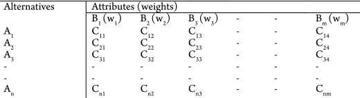
Step 1: Compute the decision matrix
Table 1
Decision Matrix Table in MADM Methods
Alternatives Attributes (weights)
B1 (w1) B2 (w2) B3 (w3) - - Bm (wm)
A1 C11 C12 C13 - - C14
A2 C21 C22 C23 - - C24
A3 C31 C32 C33 - - C34
- - -
-- - -
The decision table, given in Table 1, shows alternatives, Ai (for i = 1, 2, . . . , n), attributes,
Bj (for j = 1, 2, . . . , m), weights of attributes,
wj (for j = 1, 2, . . . , m) and the measures of
performance of alternatives, Cij (for i = 1, 2,
. . . , n; j = 1, 2, . . . , m). Given multi attribute decision making method and the decision table information, the task of the decision maker is to find the best alternative and/ or to rank the entire set of alternatives. To consider all possible attributes in decision problem, the elements in the decision table must be normalized to the same units.
Step 2: Compute the normalized decision matrix: The attributes can be considered as beneficial or non-beneficial. Normalized values are calculated by (Cij)K/(Cij)L, where
(Cij)K is the measure of the attribute for the
Kth alternative, and (C
ij)L is the measure of
the attribute for the Lth alternative that has
the highest measure of the attribute out of all alternatives considered. This ratio is valid for beneficial attributes only. A beneficial attribute (e.g., efficiency) means its higher measures are more desirable for the given decision-making problem. By contrast, non-beneficial attribute (e.g., cost) is that for which the lower measures are desirable, and the normalized values are calculated by (Cij)L/(Cij)K.
Step 3: Assuming M attributes, the pair-wise comparison of attribute i with attribute j yields a square matrix where bijdenotes
the comparative importance of attribute i with respect to attribute j. In the matrix, bij =
1 when i = j and bji = 1/bij. The judgments are
entered using the fundamental scale of the analytic hierarchy process (Triantaphyllou, 2000; Saaty, 1980).
Table 2
Saaty’s 1–9 Scale of Pair Wise Comparison
Intensity of importance Definition
1 Equal importance
3 Moderate importance
5 Strong importance
7 Very strong importance
9 Extreme importance
2 4 6 8 Intermediate values
Find the relative normalized weight (wj)
of each attribute by (a) calculating the geometric mean of the i-th row, and (b) normalizing the geometric means of rows in the comparison matrix. This can be represented as:
(1)
(2)
The geometric mean method of AHP is commonly used to determine the relative normalized weights of the attributes, because of its simplicity, easy determination of the maximum Eigen value, and reduction in inconsistency of judgments.
A2 = [w1, w2, ….. , wj]T. where A1 is
relative importance matrix.
b. Determine the maximum Eigen value λmax that is the average of matrix A4.
c. Calculate the consistency index CI =
(λmax - M) / (M - 1). The smaller the value of CI, the smaller is the deviation from the consistency.
d. Obtain the random index (RI) for the number of attributes used in decision making. Refer to Table 3 for details.
Table 3
Random Index (RI) Values
Attributes 3 4 5 6 7 8 9 10
RI 0.52 0.89 1.11 1.25 1.35 1.4 1.45 1.49
a. Calculate the consistency ratio CR = CI/RI. Usually, a CR of 0.1 or less is considered as acceptable, and it reflects an informed judgment attributable to the knowledge of the analyst regarding the problem under study.
Step 4: The next step is to obtain the overall or composite performance scores for the alternatives by multiplying the relative normalized weight (wj) of each attribute
(obtained in step 3) with its corresponding normalized weight value for each alternative (obtained in step 2), and summing over the attributes for each alternative is computed as Eq. (3):
(3)
Where (Cij) normal represents the normalized
value of Cij, and Pi is the overall or composite
score of the alternative Ai. The alternative
with the highest value of Pi is considered as
the best alternative.
4. Selection of Study Area
The study area selected for performing the present research comprises Nagpur city,
the second capital of Maharashtra state and major administrative, commercial, medical and educational center of central India. The city is experiencing the common traffic problems as most of cities of developing countries are facing i.e. rapid increase in number of vehicles, increased traffic volume compared to capacity of the road, increase in number of trips, heterogeneous traffic, roadway parking, mixed land-use along the road, encroachments and pedestrian movement on road etc.
The heavy migration of people from all the parts of country is aggregating the traffic problem. It is estimated that population of city will be about 40 lacks by 2021.
The study area selected is 217.56 sq. km located within municipal corporation boundary. The road network of Nagpur city is divided in 10 zones comprises of 72 wards designated as number 1 to 72 consist of nodes and links.
Fig. 1.
Road Network of Nagpur City
4.1. Traffic Field Study and Surveys
The field work is carried out invariably under perfect weather condition on normal working day in the month of January-February 2014. Field work is carried out in two parts: (A) Travel time study and (B) Traffic volume count.
For conducting travel time study, the test car technique is adopted. Test car was run on major traffic links in peak hours and non- peak hours. The average speed, travel time and distance between intersections
was observed and tabulated. The timing of field work was from 9.30 am to 11.30 am during morning peak hour and 5.30 pm to 7.30 pm during evening peak hours. Test car was made to run on road network between 7 am to 9 am and 12 noon to 5 pm to record travel time in non-peak hours. During the study, the test car was run at speed which in the opinion of driver is the representative of average speed of all the vehicles in stream of flow at the time of run.
hours of the day. Number of vehicles passing over the total 215 no. of links was noted in to and fro direction separately in designed tally sheet.
In addition to above, detailed surveys were conducted for collecting primary information regarding road width, number of intersections, parking and encroachment along roadway etc.
4.2. Weight Estimation Using AHP
In this section weight estimation using AHP is provided, where first dependency matrix is created based on Saaty’s scale. Referring to matrix A1, every attribute is compared with others, ex. DT (Distance) first compared with itself so value is 1, then DT is compared with TT (Travel Time) as in this case TT is moderately important than DT is value will be 1/3, when DT is compared with PCU (Traffic Volume), in this case DT is moderately important than PCU thus its value will be 3. Accordingly weight estimation is carried out by knowing the importance of individual attribute in real transportation network.
Where DT is Travel Distance, TT is Travel Time, PCU is Traffic Volume in Passenger Car Unit, RW is Road Width, NI is Number of Intersections, PR is Parking on Road and ENR is Encroachment along road.
λmax = 7.5902 CI = 0.0984 CR = 0.0729
4.3. Shortest Path between Specified
Zones
Dijkstra’s algorithm solves the single-source shortest-path problem when all edges have non-negative weights. Let G= {V, E} be a directed weighted graph with V having the set of vertices. The special vertex s in V, where s is the source and let for any edge e in E, Edge Cost(e) be the length of edge e. For the weighted directed graph its adjacency matrix A = (aij)n x n is defined as Eq. (4):
(4)
where Wij denotes the weight of arc <Vi, Vj>, ∞ denotes that there is no edge between Vi and Vj (Dijkstra, 1959).
The main steps of the Dijkstra’s algorithm are as follows (Dijkstra, 1959),
1. Use adjacency matrix C to store network information. Cij denotes the weight of arc < Vi, Vj >. If there is no arc between Vi and Vj, then Cij is set to ∞. di is defined as the weight from the source points to node Vi. Initialize starting point as ds = 0 and Di = si.
2. Select Vp, then we have,
(5)
Vp is the end point in the shortest path starting from the source point Vs. Then,
Set the end point to Vt. If Vp is equal to Vt, which means dp is the shortest path from starting point Vs to end point Vt, then algorithm stops. Otherwise, turn to step 3.
3. Modify the length of the shortest path from Vs to any point Vt in set of (V - S), and sadisfy dpas follow:
(7)
where lkp is the direct distance from point kto point j.
4. Repeat step 2 and step 3, until the shortest path is found from starting point Vs to end point Vt.
Table 4
Shortest Path over Specified Zones
Criteria for shortest path Path (Intersection Node No.) Source Zone: 4
Destination Zone: 69
Distance 4 224 223 228 227 204 170 203 97 107 202 131 132 201 200 69
Travel Time 4 92 91 90 89 88 87 76 75 74 73 127 128 129 130 136 131 132 201 200 69
PCU 4 92 192 193 194 83 195 163 196 197 198 153 152 144 151 141 142 69
Road width 4 92 191 190 180 189 105 114 188 117 187 124 186 185 132 201 200 69
Parking on road 4 92 192 193 194 83 195 163 196 197 198 153 152 144 143 142 69
Encroachment 4 92 192 193 194 83 195 163 196 197 198 153 152 151 141 142 69
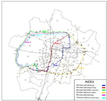
Discussion:Table 4 describes the shortest
path obtained for individual traffic attribute criteria’s like Travel Distance, Travel Time, Traffic Volume in PCU, Road Width, Parking on Road, Encroachment along link for
source zone no. 4 to destination zone no. 69. The six individual paths are obtained w.r.t. respective attribute as shown in Fig. 2 using Dijkstra’s algorithm. AHP is modeled to get best path out of six identified paths.
Fig. 2.
4.4. Optimal Path Using AHP
After obtaining shortest path between two specified zones (Zone No. 4-69) w.r.t. individual seven attribute using
Dijkstra’s algorithm, the question of complex decision making comes into action thus Analytic Hierarchy Process (AHP) is modeled for choosing the best suited path.
Table 5
Optimal Path over Specified Intersections Using AHP
Source Zone: 4 Destination Zone: 69
Alternatives AttributesDT TT PCU RW NI PR ENR AHPScore Rank
Path1 11.6 2289 24156.15 1.938024 14 44 40 0.8179 1
Path2 12.24 1540 48624.5 1.557578 19 62 59 0.7939 2
Path3 23.8 3023 20966.27 1.44524 16 30 32 0.6827 5
Path4 18.3 2437 34443.9 1.000002 16 46 43 0.6435 6
Path5 22.4 2879 21380.6 1.273018 15 29 31 0.6993 3
Path6 23.4 2969 22520.47 1.378573 15 29 30 0.6936 4
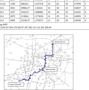
Optimal Path using AHP
Path 1: 4 224 223 228 227 204 170 203 97 107 202 131 132 201 200 69
Source Zone 4
Source Zone 69
Optimal Path
Fig. 3.
Diagram of Optimal Path Obtained Using AHP
Discussion:Table 5 describes the optimal
path obtained by considering all seven traffic attributes. AHP is modeled to obtain the optimal path. Paths which are obtained in
width, no. of intersection, parking along road and encroachment on road are considered. Table 5 provides the corresponding score for individual alternative (path) and ranking, the path which is having highest score is considered as optimal path. Fig. 3 shows the optimal path obtained between zone no. 4 to zone no. 69. In this case Path 1 is ranked as optimal path as the score of this path using AHP is found highest thus the said path may be selected as most suitable path considering the traffic condition in real traffic network between specified zones.
5. Conclusion
A useful routing system should have the capability to support the driver effectively in deciding on an optimum route to his/her preference. In this research paper, shortest path over specified zones using individual traffic attribute criteria’s like travel distance, travel time, traffic volume (PCU), road width, number of intersections, parking on road, encroachment are considered and also AHP is modeled to obtain the optimal path by considering above mentioned traffic attributes over specified zones. Using this model, optimal path between various zones of Nagpur city is found out. An example for source zone no. 4 to destination zone no. 69 is illustrated in the paper.
For the present case study, the Consistency Ratio obtained for AHP is 0.0729 which is much less than 0.1, thus optimal paths obtained using AHP for specified origin & destination zones are valid. From the experimental results for optimal path over specified zones, it is observed that in most cases the optimal path is prominently obtained for travel distance or travel time as evaluation criteria. This methodology paves the way for more intelligent traffic system.
5.1. Concluding Remarks
1. AHP is applied to route decision making process. Relative importance of each attribute in AHP is modeled. A case study of real time traffic network in Nagpur, India was conducted during peak hour period. Impacts were estimated by the aid of detailed data collected during real time traffic condition by expert team and AHP model developed.
Composite weighted AHP scored were used to generate AHP decision surface. Finally, the best decision was proposed by generating a least cost path which is most socially preferable.
2. Each objective could be represented by attributes which are either quantifiable or unquantifiable. In this study, the relative importance of quantifiable attributes such as the travel distance, travel time, traffic volume, road width, no. of intersections etc., were modeled using their relative level to standards.
For the relative importance of unquantifiable attributes such as parking condition and encroachments on road AHP was applied.
Recommendations for further studies are:
1. This study applied maximum total social benefits as a decision rule. However, applying different decision criteria may result in different solution.
2. The characteristic of response function of various impacts should be further studied.
References
Dijkstra, E.W. 1959. A note on two problems in connexion with graphs, Numerische Mathematik, Springer, 1(1): 269-271.
Dubey, S.K.; Mishra, D.; Arkatkar, S.S.; Singh, A.P.; Sarkar, A.K. 2013. Route Choice Modelling Using Fuzzy logic and Adaptive Neuro-fuzzy, Modern Traffic and
Transportation Engineering Research, 2(4): 11-19.
Hwang, C.L.; Yoon, K.P. 1981. Multiple attribute decision
making: methods and applications, Springer. 225p.
Nosal, K.; Solecka, K. 2014. Application of AHP Method for Multi-criteria Evaluation of Variants of the Integration of Urban Public Transport, Transportation
Research Procedia, 3: 269-278.
Parbat, D.K. 2001. Development of O-D Time-Distant Plot and Isochron Map for Indore city, Indian Highways, 29(9): 17-27.
Piantanakulchai, M.; Saengkhao, N. 2003. Evaluation of alternatives in transportation planning using multi-stakeholders multi-objectives AHP modeling. In
Proceedings of the Eastern Asia Society for transportation
studies, 1613-1628.
Pogarčić, I.; Davidović, V. 2008. Application of AHP method in traffic planning. In Proceedings of the 16th
International Symposium on Electronics in Traffic.
Qu, L.; Chen, Y.; Mu, X. 2008. A Transport Mode Selection Method for Multimodal Transportation Based on an Adaptive ANN System. In Proceedings of the Natural
Computation, ICNC ‘08. Fourth International Conference,
vol. 3: 436-440.
Ramazani, H.; Shafahi, Y.; Seyedabrishami, S.E. 2010. A Shortest Path Problem in an Urban Transportation Network Based on Driver Perceived Travel Time,
Transaction A: Civil Engineering, 17(4): 285-296.
Rao, R. 2007. Decision Making in the Manufacturing Environment Using Graph Theory and Fuzzy Multiple
Attribute Decision Making, Springer Series in Advanced
Manufacturing. 371 p.
Rao, R . 2013. Decision Making in Manufacturing Environment Using Graph Theory and Fuzzy Multiple Attribute
Decision Making Methods, Springer Series in Advanced
Manufacturing. 291 p.
Rardin, R.L. 2003. Optimization in Operations Research, Pearson Education, Delhi, India.
Saaty, T.L. 1980. The analytic hierarchy process, planning,
priority setting, resource allocation, New York: Mc Graw Hill.
Sadeghi-Niaraki, A.; Kim, K.; Varshosaz, M. 2010. Multi-Criteria Decision-based Model for Road Network Process, International Journal of Environmental Research, 4(4): 573-582.
Satty, T.L. 1995. Transport Planning with Multiple Criteria: The Analytic Hierarchy Process Applications and Progress Review, Journal of Advanced Transportation, 29(1): 81-126.
Triantaphyllou, E. 2000. Multi-criteria decision making
methods: a comparative study, Springer. 265 p.
Wei, T.; Zhixiang, F.; Qingquan, L. 2010. Exploring time varying shortest path of urban OD Pairs based on floating car data. In Proceedings of the 18th International
Conference on Geoinformatics, 1-6.
Yedla, S.; Shrestha, R.M. 2003. Multi-criteria approach for the selection of alternative options for environmentally sustainable transport system in Delhi,
Transportation Research Part A: Policy and Practice, 37(8):
717-729.
Zhan, F.B.; Noon, C.E. 1998. Shortest Path Algorithms: An Evaluation Using Real Road Networks, Transportation