Fields
Roberto C. Alamino and David Saad
Neural Computing Research Group, Aston University, Birmingham B4 7ET, UK
PACS numbers: 02.10.Yn, 02.70.-c, 05.10.-a
1. Introduction
Random matrices are ubiquitous in many branches of the natural sciences and mathematics ranging from biology to computer science, nuclear physics and quantum chaos. Activity in the area has been recently boosted by the application of techniques originated in the statistical mechanics of disordered systems [1, 2, 3, 4, 5, 6]. These techniques have been used to analyse ensemble properties, including variational techniques and the replica method, have proved to be valuable tools in several of these approaches. Most of the research concentrates on real matrices, while the restriction to matrices over GF(q) considered here makes the solution of the problem more involved. Random matrices over GF(q) are specially important in coding theory [7] where, for instance, linear codes are defined by the kernel of the so-called parity-check matrix: each kernel vector defines a codeword to which the original message vector is mapped by a linear operation, in the form of a product with a generator matrix. Well known examples include the Hadamard codes, where properties of the kernel and rank play an important role [8], and low-density parity-check codes (LDPC), which provide the best performance to date in many noise regimes; parity-check matrices are constructed using a special case of the sparse matrices studied here. Although the most studied and applied case of LDPC codes is of binary codes over GF(2) there is a significant body of work, of both practical and theoretical nature [9], on codes over more general finite fields showing an improvement in performance with respect to the binary version. A statistical physics based analysis of LDPC codes over GF(q) has been reported, for instance, in [10].
In addition to being an interesting applied problem, properties of these matrices are of great interest from the pure mathematical point of view and a number of papers have already addressed related questions, in different instances, with a mathematical rigorous approach [11, 12, 13].
Here, we analyse key typical properties of sparse random matrices over GF(q), namely the average dimension of their kernel, the average dimension of the eigenvector spaces, the eigenvalue distributions and the number of matrices for a given connectivity distribution, all in the case of large matrices. When the M ×N matrices are large, keeping N → ∞ with η = M/N constant, the problem can be mapped into a system of interacting “spins” by a very useful group homomorphism, and the powerful methodology developed for the study of disordered spin lattices in condensed matter physics can then be used, under some assumptions, to obtain the required properties.
random graphs. We present a final discussion of the results in section 8.
2. Generalised Mapping of GF(q) onto Spin Systems
A Galois field GF(q) is a finite field with q elements, i.e., a set of q elements {0, ..., q−1}, which we symbolise by integers for convenience, which is a commutative group under addition ⊕ : GF(q) → GF(q), defined as integer addition mod q, and with a monoid structure with respect to a commutative multiplication operation ⊗:GF(q)→GF(q). The field also includes the zero element ’0’ and the multiplicative identity ’1’. The additional requirement that both multiplication and addition have the algebraic distributive property restricts the number of elements to q=pn, where p is a prime number and n an integer.
In statistical physics applications to information theory, it is usually convenient to map binary vectors with entries from the set {0,1}, into what we call “spin” vectors with entries from the set {±1}. Given an entry v ∈ {0,1}, this mapping is usually accomplished either by the transformationσ(v) = 2v−1 or byσ(v) = (−1)v. Note that these two transformations are different in the sense that in the former, 0 is mapped to -1 and 1 is mapped to 1, while in the latter the order is reversed. The second mapping is much more convenient as it represents a homeomorphism between representations of GF(2). A further advantage, which we show below, is that this map can also be generalised to any GF(q) allowing the straightforward use of statistical physics techniques to a wide range of problems over Galois fields.
The main fact to be noted is that, under the operation of addition ⊕, GF(q) is homeomorphic to the cyclic group of order q and therefore has a representation as the complex q-th roots of unity with the group homeomorphism σ:GF(q)→Cgiven by
σ(v) = exp
2πi q v
, (1)
such that for every v1, v2 ∈GF(q)
σ(v1⊕v2) = exp
2πi
q (v1⊕v2)
= exp
2πi
q (v1+v2)
=σ(v1)σ(v2).
(2)
This mapping has a clear geometric interpretation where 2πv/q is an angle in the unit circle, such that each element of the Galois field is being mapped onto a spin variable “pointing” in one of q possible directions. Let us denote the inverse of an element v
under addition by−v such that v⊕(−v) = 0. Then we also have
σ(v⊕(−v)) =σ(0) = 1⇒σ(−v) = [σ(v)]−1, (3)
In several applications, including the ones studied in this paper, it turns out to be necessary to use constraints in the form of Kroenecker deltas like
δ(v, u) = δ(v⊕(−u),0). (5)
Using the above mapping, one can write any constraint of this type in a generalised way as
δ(v, u) = 1
q
q−1
Y
m=1
1−exp
−2πi
q m
exp
2πi q v
exp
−2πi
q u
. (6)
Also based on this representation, we can now define the k-point functions of the spins by
mk ≡ 1
N
N
X
j=1
σ1j· · ·σkj, (7)
where the lower indices representkdifferent spin configurationsσ1, ...,σk. Note that we
are now working with the spin variables already mapped onto the complex field C and
therefore the operations of multiplication and addition correspond to the usual ones on
C. The first twok-point functions, namelym1 andm2, correspond to the magnetisation
of the spin system and its overlap between two configurations, respectively.
As will become evident in what follows, this kind of representation allows a factorisation of terms that simplifies the equations and makes replica calculations simpler.
3. Kernel and Rank
Entries in matrices overGF(q) take values of elements of that finite field, where the usual additions and multiplications involved in their algebra are defined by the corresponding operations over the Galois field.
The kernel of an M ×N matrix A over GF(q) is a linear space with dimension
dA(0) = logqΩA(0) where
ΩA(0) =X
v
δ(Av,0), (8)
is the number of vectors in the kernel, δ is the Kroenecker delta and v∈GF(q)N. We termT s(0) theaverage kernel dimension density, in the limit of large matrices, where we also define the entropy density
s(0)≡ 1
T Nlim→∞
hdA(0)iA
N = limN→∞
1
Nhln ΩA(0)iA, (9) with 1/T = lnq and with the ratio η = M/N being a finite positive constant and h·iA denotes an average over the corresponding ensemble of random matrices. Using the replica trick we can write the entropy density as
s(0) = lim N→∞
∂ ∂nlnhΩ
n A(0)iA
n=0
We focus our analysis on the class of randomly chosen sparse matrices A having exactlyKi non-zero elements in the i-th row with probabilityP(K),K≡(K1, ..., KM), and Cj elements in the j-th column with probability P(C), C≡ (C1, ..., CN), obeying the constraint Λ ≡ P
iKi =
P
jCj, where Λ is the total number of non-zero elements of the matrix. We also consider that the elements ofA are sampled from the finite field
GF(q) with independent equal probabilities P(Aij).
Using the mapping ofGF(q) into spin variables defined in the previous section, the replicated averaged partition function Zn(0)≡ hΩn
A(0)iA can be written as
Zn(0) =
*
1 N
X
{Aij}
" Y
i,j
P(Aij)
#"M Y
i=1
δ
N
X
j=1
χ(Aij), Ki
!#" N Y
j=1
δ
M
X
i=1
χ(Aij), Cj
!#
× n
Y
a=1
" X
va
δ(Ava,0)
#+
K,C,Λ
,
(11)
where the average is over the probability distribution P(K,C,Λ) with χ(Aij) = 0 if Aij = 0 and 1 otherwise, and the normalisation N gives the number of matrices which obey the constraints averaged over the distributions of the entries. The replica calculations to obtain the entropy (9) have already been carried out in a previous paper [14] and we will only discuss the important results. One important difference of this approach in comparison to previous similar calculations [15, 16] is that, instead of defining connectivity tensors and summing over them, here and in [14] we sum directly over the matrices entries, which makes possible to include general constraints over the class of random matrices.
Using the rank-nullity theorem, we can define the free energy density f(0) as the
average rank density in the form
f(0)≡ hr(A)iA
N = 1−T s(0), (12)
which implies that the internal energy density of the associated statistical mechanical model should be constrained to be u = 1. Defining the inverse temperature β = 1/T, equation (12) can be written as
βf(0) =−1
N
*
lnX
v
e−βH(v)
+
A
, (13)
where a formal Hamiltonian can be written as
H(v)≡N −lnδ(Av,0). (14)
0.0 0.5 1.0 λ
0.0 0.5 1.0
Kernel Dimension Rank
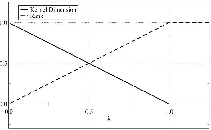
Figure 1. Average kernel dimension density (continuous lines) and average rank density (dashed lines) calculated as solutions to the replica symmetric saddle point equations. The plot shows the thermodynamically favoured analytical solution which is paramagnetic for 0≤η≤1 and ferromagnetic forη >1.
of Λ). Analytical solutions cannot be obtained in general and we must rely on numerical methods to obtain them. However, there exists two straightforward analytical solutions, the paramagnetic and ferromagnetic states. The paramagnetic solution gives the average kernel density as T s(0) = 1−η = 1−M/N independently of the order q of the finite field used, and the ferromagnetic solution gives simply T s(0) = 0. Figure 1 shows a plot of the thermodynamically dominant solutions for varying η. We see that the paramagnetic solution dominates until η = 1, after which it becomes unphysical and the correct solution is given by the ferromagnetic one.
In [14], numerical solutions for three different distributions of K, C and Λ were thoroughly studied and, apart from small variations resulting from particular properties of the distributions, the obtained curves seem to reproduce figure 1.
4. Error Correcting Codes
Low-density parity-check codes are linear codes where the codewords are defined by the kernel of a random sparse matrix, called the parity-check matrix. In most studies of LDPC codes, it is assumed that a parity-check matrix with M rows (parity-checks) and
N columnsexactly defines a code of rate R= 1−M/N = 1−η, which is equivalent to the assertion that the number of codewords (vector in the kernel) is exactly qN R.
The results of the previous section give us a method to rigorously test this assertion. Note that when M ≥ N, the code rate, in the case of unbiased messages, would be negative, which is unphysical. However, our calculations give a clear interpretation for this case as they show that ifη >1, the dominant solution is the ferromagnetic one with
the zero message, this incidentally means that such matrices cannot be used to define a parity-check code due to the lack of redundancy.
However, when η < 1, the dominant solution is paramagnetic and the typical parity-check matrix defines a code of rate exactly (N−M)/N. This is assumed for any parity-check matrix in most calculations in the literature and is confirmed by our results to be true on average; however, it is important to point out that the result is true in the limit of large matrices and is likely to have finite size corrections which may affect practical applications.
The application to error correcting codes also gives support to our conjecture that the dominant solution for η < 1 is the paramagnetic one and for η ≥ 1 it is the ferromagnetic solution for any distribution. The argument is that the solution of the kernel dimension is mathematically equivalent to the solution of LDPC in channels with infinite noise, which then leads to this behaviour. As already mentioned, the numerical results of [14] seem to support this conjecture, although more careful calculations, varying all the parameters involved must be carried out to confirm this hypothesis more generally.
5. Eigenspaces and Eigenvalues
In the case of square M × M matrices, which means that η = 1, we can generalise equation (8) to count the number of vectors in an eigenspace with eigenvalue λ ∈ {1, ..., q−1} as
ΩA(λ) =X
v
δ(Av, λv), (15)
with obvious analogous generalisations for the kernel dimension density dA(λ), its average density T s(λ) and all other quantities from section 3 that depend on λ, the free energy now being the dimension of the complementary space to the λ-eigenspace.
The replica calculations are very similar to the particular case of the kernel [14]. However, as there are key differences and in order to keep this paper as self-contained as possible, we reproduce the replica calculations including the appropriate changes to the eigenspace case in Appendix A. The replica symmetric solution, exact for this problem as shown in Appendix B, is therefore (for λ6= 0)
s(λ) = −lnq− α
Mhln [1 + (q−1)xxˆ]ix,xˆ
+ 1
M ǫ(α)
X
i
*
αΛ
Λ!
*
ln
("
1 + (q−1) Ki
Y
l=1
xl
# Ci Y
l=1
[1 + (q−1)ˆxl]
+ (q−1) 1− Ki
Y
l=1
xl
! Cj
Y
l=1
(1−xˆl)
+
x,xˆ
+
K,C,Λ
,
(16)
than in the kernel case and are given by the saddle point equations
ˆ
π(ˆx) = 1
αǫ(α) M
X
i=1
αΛ
Λ!Ki
×δ xˆ−
"Ki−1 Y
l=1
xl
#
ˆ
X+(Ci)−Xˆ−(Ci)
ˆ
X+(C
i) + (q−1) ˆX−(Ci)
!+
ˆ x,K,C,Λ
, (17)
π(x) = 1
αǫ(α) M
X
i=1
αΛ
Λ!Ci
×δ x− X
+(Ki) ˆX+(C
i−1)−X−(Ki) ˆX−(Ci−1)
X+(Ki) ˆX+(C
i −1) + (q−1)X−(Ki) ˆX−(Ci−1)
!+
ˆ x,K,C,Λ
, (18)
0 =
αΛ
Λ!
1− Λ
α
K,C,Λ
, (19)
with the following definitions for simplicity
ǫ(α)≡
αΛ
Λ!
K,C,Λ
, (20)
ˆ
X+(C)≡ C
Y
l=1
[1 + (q−1)ˆxl], Xˆ−(C)≡ C
Y
l=1
(1−xˆl), (21)
X+(K)≡1 + (q−1) K
Y
l=1
xl, X−(K)≡1− K
Y
l=1
xl. (22)
The paramagnetic solution
ˆ
π(ˆx) = δ(ˆx), π(x) =δ(x), (23)
and the ferromagnetic solution
ˆ
π(ˆx) = δ(ˆx−1), π(x) =δ(x−1). (24)
in terms of the auxiliary fields are the same as for the kernel. Substituting these solutions into equation (16), we see that the paramagnetic solution gives the result s(λ) = 0 for every value of λ, which must be discarded as the kernel calculation shows thats(0) = 0 in the square matrix case. The matrix is therefore diagonalisable and the dimension of the eigenspaces cannot be zero. On the other hand the ferromagnetic solution gives
s(0) = 0 ands(λ) = Λ/M forλ6= 0, which means that all the non-zero eigenvalues have eigenspaces with the same dimension given by the average value of non-zero entries per row or per column (both must be equal). As Λ scales with M; it gives a finite average dimension density as expected. This result also implies that the eigenvalue distribution is just given by
6. Number of Matrices
The number ofGF(q) matrices given a connectivity profile is of significant interest within the discrete mathematics community. Exact results have been obtained for the case of
finitebinary matrices [17] in the form of a formula that facilitates the calculation of their precise number. Using the same techniques from the previous sections, this number and its average value can be obtained for largeGF(q) matrices. For a given number of non-zero elements per row K= (K1, ..., KM) and per column C= (C1, ..., CN), the number of matrices is
NA=
X
{Aij}
"M Y
i=1
δ
N
X
j=1
χ(Aij), Ki
!#" N Y
j=1
δ
M
X
i=1
χ(Aij), Cj
!#
, (26)
where again we are summing directly over the entries of the matrix instead of over a connectivity tensor. The detailed calculations where presented in [14] resulting in
NA= (q−1)Λ
Λ!
Q
iKi!
Q
jCj!
, (27)
which is just the number of binary matrices with the given non-zero elements profile times a factor (q−1)Λ which is the multiplicity of the non-zero entries.
The average number of matrices is then
¯
NA =
*
(q−1)ΛQ Λ!
iKi!
Q
jCj!
+
K,C,Λ
=X
K
X
C
P(K|C)P(C)(q−1)PjCj
P
jCj
!
Q
iKi!
Q
jCj!
,
(28)
where the distribution P(K|C) includes the constraintδP
iKi,PjCj
. For a regular matrix, it is easy to see that this number scales asNCN and a more appropriate quantity would be the quenched entropy
Ξ≡
1
N lnNA
= 1
N
X
K
X
C
P(K|C)P(C) ln
(q−1) P
jCj
P
jCj
!
Q
iKi!
Q
jCj!
, (29)
scaling as lnN.
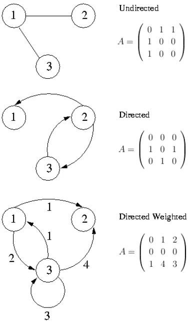
Figure 2. Examples of adjacency matrices. From top to bottom, undirected graphs, directed graphs and directed weighted graphs.
7. Random Graphs
The results of the previous section can be used to obtain the number and average number of generalised sparse random graphs. For usual random graphs, directed or undirected, the adjacency matrix can be written as a binary matrix with a 1 in entry Aij if there is a link from vertex i to vertex j. If in addition each link is given an integer weight, the matrix can be viewed as a GF(q) matrix for the sake of counting the graphs. In figure 2, we give an example of a directed, an undirected and an undirected weighted graph.
Graphs like the ones in figure 2 can be used in statistical physics to describe systems with 2-body interactions, like an Ising model, for instance. However, there exists systems with many-body interactions and we would like to be able to describe them by graphs and matrices as well. With this in mind, we can generalise random graphs in the following way. Instead of only links that connect two vertices, representing an interaction between them, we allow for the existence of polygons connecting p ≥3 vertices with a
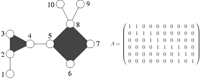
Figure 3. Example of a graph withp-spin interactions and its matrix representation.
row carries the label of the vertices. This is the type of representation frequently used in most studies of codes [18]. An example of such a graph is given in figure 3. In fact this is a matrix representation of the tensor whose indices identify the interacting variables. In this way, we can represent any interacting system as a random GF(q) matrix, which allows us to use the results of the former section to calculate their number or their average number according to our needs.
8. Conclusions
The main object of this work was to study some typical properties of sparse random matrices over Galois fields using techniques originated in the statistical physics of disordered systems.
In order to carry on our analysis, we introduced a mapping from Galois matrices to spin systems based on the group homeomorphism between GF(q) under addition mod q (denoted by ⊕) and the complex q-th roots of unity. This mapping allows for a direct analogy between the matrices and statistical mechanical systems in the canonical ensemble, making it possible to associate properties like rank and nullity with thermodynamical characteristic functions like the free-energy and entropy.
The key point, which is the calculation of the quenched entropy, was carried out in a set up that allows for further generalisations of the constraints enforced in defining the classes of matrices over which the averaging is done by characterising their connectivity profiles. This quenched average is carried out using the replica approach and we are able to obtain, as a result, the average dimension of the kernel for a general distribution of non-zero entries. Solving the resulting equations numerically, we find that the average kernel density is 1−M/N in all cases studied. We conjecture that this result is always valid. The replica symmetric ansatz was assumed in the calculation and later on proved to be exact in this case with the help of the mapping between matrices and spin systems; this sheds light on the meaning of properties like magnetisation and spin correlation.
implies that randomly generated LDPC codes typically define codes of rate exactly 1−M/N, an assumption which is generally made but lacks rigorous derivation.
A generalisation of the result for the kernel and rank allowed us to obtain the dimension of each eigenspace and its corresponding eigenvalue distribution.
By using the same mathematical techniques, we were also able to find the total number of large matrices for fixedKandC, row and column connectivities, respectively, and their average number. We showed then how the matrices could be used to represent not only usual graphs, but also the connectivity profile of graphs representing p -spin interactions. The results obtained for the average number of matrices provide therefore a principled approach to determine the average number of possible graphs with given connectivity distributions of a more general nature than the connectivity profiles examined in this paper.
Extensions and generalisations of the presented framework are under study. A most desired generalisation would be to continuous matrices. The first step in this direction is to study matrices with entries in continuous groups instead of the elements of a finite group, more specifically, U(1) which is a straightforward continuous limit of the cyclic groups.
Acknowledgements
Support from EPSRC grant EP/E049516/1 is gratefully acknowledged. R.C.A. would also like to thank Juan P. Neirotti and Jack Raymond for useful discussions.
References
[1] Mezard, M., Parisi, G., and Zee, A. Nucl. Phys. B559, 689–701 (1999). [2] Kanzieper, E. Nucl. Phys. B596, 548–566 (2001).
[3] Nagao, T. and Tanaka, T. J. Phys. A40, 4973–4987 (2007).
[4] Biroli, G., Bouchaud, J.-P., and Potters, M. Europhys. Lett.78, 10001 (2007). [5] Biroli, G., Bouchaud, J.-P., and Potters, M. J of Stat. Mech., P07019 (2007). [6] Bohigas, O., de Carvalho, J. X., and Pato, M. P. Phys. Rev. E77, 011122 (2008).
[7] McEliece, R. Theory of Information & Coding. Cambridge University Press, Cambridge, MA, (2002 2nd edition).
[8] Phelps, K. T., Rif`a, J., and Villanueva, M. IEEE Trans. Inf. Theory51, 3931–3937 (2005). [9] Davey, M. and MacKay, D. IEEE Communications Letters2, 165 – 167 (1998).
[10] Nakamura, K., Kabashima, Y., and Saad, D. Eurphys. Lett.56, 610–616 (2001). [11] Cooper, C. Random Structures and Algorithms16, 209–232 (2000).
[12] Bl¨omer, J., Karp, R., and Weiz, E. Random Structures and Algorithms10, 407–419 (1998). [13] Feng, X. and Zhang, Z. App. Math. and Comp.185, 689–694 (2007).
[14] Alamino, R. C. and Saad, D. Phys. Rev. E77, 061123 (2008).
[15] Alamino, R. C. and Saad, D. J. Phys A: Math. Theor.40, 12259–1279 (2007). [16] Yano, T., T[]Tanaka, and Saad, D. J Phys A41(32), 324022 (15pp).
[17] Wang, B.-Y. and Zhang, F. Discrete Mathematics187, 211–220 (1998).
[19] Nishimori, H. Statistical Physics of Spin Glasses and Information Processing. Oxford University Press, Oxford, UK, (2001).
Appendix A. Replica Calculations
For the case square matrices (η= 1) and λ 6= 0, we can use the integral representation of the Kroenecker delta function in the complex plane such that the averaged replicated kernel size defined in equation (11) is generalised to the size theλ-eigenspace as
Zn(λ) =
*
1 N
X
{va}
I
DW DZ X
{Aij}
" Y
i,j
P(Aij)(WiZj)χ(Aij)
# × M Y i=1 Y a δ " M M j=1
Aij ⊗vaj
, λ⊗vi a
#+
K,C,Λ
,
(A.1)
where ⊗ and ⊕indicate respectively multiplication and summation on GF(q) and
DW DZ =
" M Y
i=1
dWi
WKi+1
i
#"M Y
j=1
dZj
ZCj+1
j
#
. (A.2)
Using the representation of the Kroenecker delta given in equation (6), the product over replica indices of the delta function can be written as
Y a δ " M M j=1
Aij ⊗vja
, λ⊗vi a # =Y a 1 q
q−1
Y
m=1
(
1−exp
−2πi
q m
exp
−2πi
q λ⊗v
i a M Y j=1 exp 2πi
q Aij ⊗v
j a ) = 1 qn Y a " 1 + q−1
X
s=1
Fi(s, a)G(s)
# = 1 qn n X r=0 X
ha1···ari
X
s1,...,sr
G(s1)· · ·G(sr)Fi(s1, a1)· · ·Fi(sr, ar),
(A.3)
with
G(s)≡ X
hm1···msi
(−1)sexp
−2πi
q m1
· · ·exp
−2πi
q ms
, (A.4)
and
Fi(s, a) = exp
−2πi
q s λ⊗v
i a M Y j=1
γj(s, a, Aij), (A.5)
where we defined, for simplicity,
γj(s, a, Aij)≡exp
2πi
q s Aij ⊗v
j a
The partition function becomes
Zn(λ) =
*
1 N
X
{va}
I DZ M Y i=1 1 qn n X r=0 X
ha1···ari
X
s1,...,sr
G(s1)· · ·G(sr)
I
dWi 2πi
1
WKi+1
i Γi
+
K,C,Λ
,
(A.7) where
Γi = exp
−2πi
q s1 λ⊗v
i a1
· · ·exp
−2πi
q sr λ⊗v
i ar ×Y j X Aij
P(Aij)(WiZj)χ(Aij)γj(s1, a1, Aij)· · ·γj(sr, ar, Aij)
=pMexp
−2πi
q s1 λ⊗v
i a1
· · ·exp
−2πi
q sr λ⊗v
i ar ×Y j "
1 + 1
p
q−1
X
h=1
P(Aij =h)WiZjγj(s1, a1, h)· · ·γj(sr, ar, h)
#
,
(A.8)
where we define, for convenience, p ≡ P(Aij = 0). Let us define a probability distribution over the values of h as
P(h) = P(Aij =h)
1−p , (A.9)
in such a way thathvaries from 1 toq−1 and the probability over this range is correctly normalised. Then
Γi =pMexp
−2πi
q s1 λ⊗v
i a1
· · ·exp
−2πi
q sr λ⊗v
i ar ×Y j 1 +
1−p p
WiZjhγj(s1, a1, h)· · ·γj(sr, ar, h)ih
=pMexp
−2πi
q s1 λ⊗v
i a1
· · ·exp
−2πi
q sr λ⊗v
i ar N X l=0 X
hj1···jli
1−p p
l
×WilZj1· · ·Zjlhγj1(s1, a1, h)· · ·γj1(sr, ar, h)ih· · · hγjl(s1, a1, h)· · ·γjl(sr, ar, h)ih. (A.10)
we therefore obtain
Zn =
*
κX
{va}
I DZ M Y i=1 n X r=0 X
ha1···ari
X
s1,...,sr
G(s1)· · ·G(sr)
×exp
−2πi
q s1 λ⊗v
i a1
· · ·exp
−2πi
q sr λ⊗v
i ar
X
hj1···jKii
Zj1· · ·ZjKi
× hγj1(s1, a1, h)· · ·γj1(sr, ar, h)ih· · ·
D
γjKi(s1, a1, h)· · ·γjKi(sr, ar, h)
E
h
oE
K,C,Λ
≈
*
κX
{va}
I DZ M Y i=1 n X r=0 X
ha1···ari
X
s1,...,sr
G(s1)· · ·G(sr)
×exp
−2πi
q s1 λ⊗v
i a1
· · ·exp
−2πi
q sr λ⊗v
i ar × N Ki Ki! " 1 N N X j=1
Zjhγj(s1, a1, h)· · ·γj(sr, ar, h)ih
#Ki
+
K,C,Λ
(A.11)
where
κ=pM21−p p
PiKi
N−1q−nM. (A.12)
The calculation of N is similar to the calculation of the number of matrices [14] and we end up with
κ= 1
qnMN(2) A
, (A.13)
where NA(2) is exactly the number of binary matrices (q = 2). Introducing the replica overlaps
Qs1,...,sr
ha1···ari ≡
1
M
M
X
j=1
Zjhγj(s1, a1, h)· · ·γj(sr, ar, h)ih, (A.14)
and the corresponding auxiliary variables ˆQs1,...,sr
ha1···ari by means of Dirac delta functions,
run through the same set, we can express the partition function as
Zn=
Z
DQDQˆexp−MXQs1,...,sr
ha1···ari
ˆ
Qs1,...,sr
ha1···ari
×
*
κM
P
iKi
Q
iKi!
Y
i
X
{va}
X
G(s1)· · ·G(sr)
Qs1,...,sr
ha1···ari
Ki
×exp
−2πi
q s1(λ⊗va1)
· · ·exp
−2πi
q sr(λ⊗var)
×
I
DZiexp
h
Zi
X
ˆ
Qs1,...,sr
ha1···arihγi(s1, a1, h)· · ·γi(sr, ar, h)ih
i
K,C,Λ
=
Z
DQDQˆexp−MXQs1,...,sr
ha1···ari
ˆ
Qs1,...,sr
ha1···ari
×
*
q−nM M
P
iKi
(P
iKi)!
Y
i
X
{va}
X
G(s1)· · ·G(sr)
Qs1,...,sr
ha1···ari
Ki
×exp
−2πi
q s1(λ⊗va1)
· · ·exp
−2πi
q sr(λ⊗var)
×hXQˆs1,...,sr
ha1···arihγi(s1, a1, h)· · ·γi(sr, ar, h)ih
iCi
K,C,Λ
(A.15)
where
DQDQˆ ≡ Y dQ dQˆ 2πi/M
!
, (A.16)
and the summations run over all the allowed values of r,ha1· · ·ariand s1, . . . sr.
Under the assumption of replica symmetry in the form
Qs1,...,sr
ha1···ari =Q0hx
ri
x, (A.17)
ˆ
Qs1,...,sr
ha1···ari = ˆQ0hˆx
ri
ˆ
x, (A.18)
where the averages over x and ˆx are taken with respect to the field distributions π(x) and ˆπ(ˆx) respectively, we can show by straightforward algebraic manipulations that
X
Qs1,...,sr
ha1···ari
ˆ
Qs1,...,sr
ha1···ari =Q0
ˆ
Q0h[1 + (q−1)xxˆ]nix,xˆ, (A.19)
X
G(s1)· · ·G(sr)
Qs1,...,sr
ha1···ari
Ki
exp
−2πi
q s1(λ⊗va1)
· · ·exp
−2πi
q sr(λ⊗var)
=
QKi
0
* n Y
a=1
"
1 + ˜ω(va) Ki Y l=1 xl #+ x , (A.20) with ˜
ω(v)≡ q−1
X
s=1
G(s) exp
−i2πs
q (λ⊗v)
and
hX ˆ
Qs1,...,sr
ha1···arihγi(s1, a1, h)· · ·γi(sr, ar, h)ih
iCi
=
ˆ
QCi
0 * n Y a=1 Ci Y l=1
[1 +ω(va, hl)ˆxl]
+
ˆ x,h
,
(A.22)
with
ω(v, hl)≡ q−1
X
s=1
exp
i2πs
q (hl⊗v)
=
(
q−1, ifhl⊗v = 0,
−1, otherwise. (A.23)
Therefore, we have, for the sum over{va},
X
{va}
(
QKi
0
* n Y
a=1
"
1 + ˜ω(va) Ki Y l=1 xl #+ x ) ˆ
QCi
0 * n Y a=1 Ci Y l=1
[1 +ω(va, hl)ˆxl]
+
ˆ x,h
=QKi
0 Qˆ
Ci 0 *( X v "
1 + ˜ω(v) Ki
Y
l=1
xl
# Ci Y
l=1
[1 +ω(v, hl)ˆxl]
)n+
x,ˆx,h
=QKi
0 Qˆ
Ci
0
*("
1 + (q−1) Ki Y l=1 xl # C i Y l=1
[1 + (q−1)ˆxl]
+
(
(q−1) +
"q−1 X
v=1
˜
ω(v)
# K i Y l=1 xl )"C i Y l=1
(1−xˆl)
#)n+
x,ˆx ,
(A.24)
where with some amount of algebraic calculations to show that
q−1
X
v=1
˜
ω(v) =−(q−1), (A.25)
when λ6= 0, we can write
Zn=
Z
DQDQ eˆ Ms˜, (A.26)
with
˜
s =− 1
M lnN
(2)
A −nlnq−Q0Qˆ0h[1 + (q−1)xxˆ]nix,xˆ+
1
M ln Φ, (A.27)
where Φ = * MΛ Λ! Q Λ 0QˆΛ0
Y
i
*("
1 + (q−1) Ki
Y
l=1
xl
# Ci Y
l=1
[1 + (q−1)ˆxl]
+ (q−1) 1− Ki
Y
l=1
xl
! Cj
Y
l=1
(1−xˆl)
n
+
x,ˆx
+
K,C,Λ
Let us define α ≡ M Q0Qˆ0. For n ≪ 1, we can consider only the leading
contributions in the number of replicas, which gives
ln Φ = lnǫ(α) + n
ǫ(α)
X
i
αΛ
Λ!hln{· · · }ix,xˆ
K,C,Λ
, (A.29)
with
ǫ(α) =
αΛ
Λ!
K,C,Λ
, (A.30)
and where{· · · }stands for the expression inside curly brackets in equation (A.28) above. Substituting the above formulas in ˜s for n → 0, the extremization with respect to
Q0, ˆQ0,π(x) and ˆπ(ˆx) leads to the saddle point equations (17), (18) and (19).
Appendix B. Proof of Replica Symmetry
Let us consider the probability distribution inside a specific eigenspace with λ 6= 0. Then
P(v|λ) =
" X
v
δ(Av, λv)
#−1
=q−dA(λ). (B.1)
The distribution of the k-point functions is
P(mk) =
*
δ mk− 1
N
N
X
j=1
σ1j· · ·σkj
!+
σ1,...,σk
=q−kdA(λ) X
v1,...,vk
δ(Av1, λv1)· · ·δ(Avk, λvk)
×δ
"
mk− 1
N
N
X
j=1
exp
2πi
q v
j
1 +· · ·+v
j k
#
.
(B.2)
Let us call
g(v1, ...,vk)≡δ
"
mk− 1
N
N
X
j=1
exp
2πi
q v
j
1+· · ·+v
j k
#
and note that g(v1,v2, ...,vk) = g(v1,v2, ...,vk−1⊕vk,0). Therefore we can write
P(mk) =q−kdA(λ) X
v1,...,vk
δ(Av1, λv1)· · ·δ(Avk, λvk)g(v1,v2, ...,vk−1⊕vk,0)
=q−kdA(λ) X
v1,...,vk
δ(Av1, λv1)· · ·δ(Avk, λvk)
X
u
δ(u,vk−1⊕vk)g(v1,v2, ...,u,0)
=q−kdA(λ) X
v1,...,vk −2,u
g(v1,v2, ...,u,0)
×X
vk −1
δ(Avk−1, λvk−1)
X
vk
δ(Avk, λvk)δ(u,vk−1⊕vk)
=q−kdA(λ) X
v1,...,vk −2,u
g(v1,v2, ...,u,0)
×X
vk −1
δ(Avk−1, λvk−1)δ(A(u⊕(−vk−1)),0)
=q−(k−1)dA(λ) X
v1,...,vk −2,u
δ(Au, λu)g(v1,v2, ...,u,0)
=
*
δ mk− 1
N
N
X
j=1
σj1· · ·σjk−1
!+
σ1,...,σk
−1 .
(B.4)