R E S E A R C H
Open Access
Sparsity estimation from compressive
projections via sparse random matrices
Chiara Ravazzi
1*, Sophie Fosson
2, Tiziano Bianchi
3and Enrico Magli
3Abstract
The aim of this paper is to develop strategies to estimate the sparsity degree of a signal from compressive projections, without the burden of recovery. We consider both the noise-free and the noisy settings, and we show how to extend the proposed framework to the case of non-exactly sparse signals. The proposed method employsγ-sparsified random matrices and is based on a maximum likelihood (ML) approach, exploiting the property that the acquired measurements are distributed according to a mixture model whose parameters depend on the signal sparsity. In the presence of noise, given the complexity of ML estimation, the probability model is approximated with a two-component Gaussian mixture (2-GMM), which can be easily learned via expectation-maximization.
Besides the design of the method, this paper makes two novel contributions. First, in the absence of noise, sufficient conditions on the number of measurements are provided for almost sure exact estimation in different regimes of behavior, defined by the scaling of the measurements sparsityγ and the signal sparsity. In the presence of noise, our second contribution is to prove that the 2-GMM approximation is accurate in the large system limit for a proper choice ofγparameter. Simulations validate our predictions and show that the proposed algorithms outperform the state-of-the-art methods for sparsity estimation. Finally, the estimation strategy is applied to non-exactly sparse signals. The results are very encouraging, suggesting further extension to more general frameworks.
Keywords: Sparsity recovery, Compressed sensing, High-dimensional statistical inference, Gaussian mixture models, Maximum likelihood, Sparse random matrices
1 Introduction
Compressed sensing (CS) [1,2] is a novel signal acquisi-tion technique that recovers an unknown signal from a small set of linear measurements. According to CS, if a sig-nal having dimensionnis known to be sparse, i.e., it has onlyk nnon-zero entries when represented by a suit-able basis, then it can be efficiently recovered using only mnlinear combinations of the signal entries, provided that these linear projections are sufficiently incoherent with respect to the signal basis.
In most of CS applications, it is usually assumed that an upper bound on the sparsity degreekis known before acquiring the signal. However, some signals may have a time-varying sparsity, as in spectrum sensing [3], or spa-tially varying sparsity, as in the case of block-based image acquisition [4]. Since the number of linear measurements
*Correspondence:[email protected]
1National Research Council of Italy, IEIIT-CNR, c/o Politecnico di Torino, Corso Duca degli Abruzzi 24, 10129 Torino, Italy
Full list of author information is available at the end of the article
required for the recovery depends on the sparsity degree of the signal [5], the knowledge of k is crucial to fully exploit the potential of CS.
In many recovery algorithms, the optimal tuning of parameters requires the knowledge of the degree of spar-sity of the signal. For example, in Lasso techniques [6], a parameterλrelated tokhas to be chosen [7], whereas for greedy algorithms, such as orthogonal matching pur-suit (OMP) [8] or compressive sampling matching pursuit (CoSaMP) [9], the performance and the number of itera-tions depend onk.
The ability to estimate the signal sparsity degree directly from a small number of linear measurements can repre-sent an important tool in several promising applications. One of the most obvious applications is the possibility to dynamically adapt the number of measurements acquired by a CS instrument, e.g., an imager, to the estimated signal sparsity. We can envisage a system that acquires linear measurements in a sequential way and continu-ously updates the estimated sparsity according to the new
measurements. The acquisition can stop as soon as the number of acquired measurements is enough to guaran-tee the correct reconstruction of a signal based on the estimated sparsity.
Other applications may include the possibility of com-paring the support of two sparse signals from their mea-surements. Due to the linearity of the sparse signal model, the degree of overlap between the supports of two sparse signal can be estimated by measuring the sparsity degree of their sum (or difference) [10]. Finally, sparsity estima-tion can be used to decide whether a signal can be repre-sented in a sparse way according to a specific basis, which can be used to select the most suitable basis allowing the sparsest representation.
1.1 Related work
The problem of estimating the sparsity degree has begun to be recognized as a major gap between theory and prac-tice [11–13], and the literature on the subject is very recent.
In some papers, the joint problem of signal reconstruc-tion and sparsity degree estimareconstruc-tion is investigated, in particular for time-varying settings. The following itera-tive approach is considered: given an initial upper bound for the sparsity degree, at a generic time stept, the sig-nal is reconstructed and sparsity degree is estimated; such estimation is then used at timet+1 to assess the number of measurements sufficient for reconstruction. The sem-inal work [14] investigates the problem in the framework of spectrum sensing for cognitive radios and proposes an iterative method that at each time step performs two oper-ations: (a) the signal is recovered via Lasso, and (b) the sparsity degree is estimated as the number of recovery components with magnitude larger than an empirically set threshold. The efficiency of this procedure is validated via numerical simulations.
Some authors propose sequential acquisition tech-niques in which the number of measurements is dynamically adapted until a satisfactory reconstruction performance is achieved [15–19]. Even if the reconstruc-tion can take into account the previously recovered signal, these methods require to solve a minimization problem at each newly acquired measurement and may prove too complex when the underlying signal is not sparse, or if one is only interested in assessing the sparsity degree of a signal under a certain basis without reconstructing it.
In other papers, the sparsity degree estimation is only considered, which generally requires less measurements than signal reconstruction. In [13], sparsity degree is esti-mated through an eigenvalue-based method, for wide-band cognitive radios applications. In this work, the signal reconstruction is not required, while in practice, the used number of measurements was quite large. In [20], the sparsity of the signal is lower-bounded through
the numerical sparsity, i.e., the ratio between the1and 2 norms of the signal, where these quantities can be estimated from random projections obtained using Cauchy-distributed and Gaussian-distributed matrices, respectively. A limitation of this approach is that it is not suitable for adaptive acquisition since measurements taken with Cauchy-distributed matrices cannot be used later for signal reconstruction. In [21], this approach is extended to a family of entropy-based sparsity measures of kind(xq/x1)q/(1−q) withq ∈[ 0, 2], for which esti-mators are designed and theoretically estimated in terms of limiting distributions. In [22], the authors propose to estimate the sparsity of an image before its acquisition, by calculating the image complexity. However, the pro-posed method is based on the image pixel values and needs a separate estimation that does not depend on the measurements. Further, in [23], the minimum num-ber of measurements to recovery, the sparsity degree was theoretically investigated.
Finally, we notice that the problem of estimating the sparsity degree of a vector is partially connected to the problem of estimating the number of distinct elements in data streams [24, 25], which has been largely studied in the last decades due to its diverse applications. The analogy lies in the fact that the sparsity degree problem could be seen as the estimation of the number of elements distinct from zero. Moreover, many efficient algorithms to estimate the number of distinct elements are based on random hashing (see [25] for a review) to reduce the storage space, which is our concern as well. How-ever, the problem of distinct elements considers vectors a=(a1,. . .,an)withai∈Q, whereQis a finite set, which is intrinsically different from our model where the signal x has real-valued components. Therefore, the strategies conceived for this problem cannot be applied for our purpose.
1.2 Our contribution
(2-GMM), whose parameters can be easily estimated via expectation-maximization (EM) techniques. In this case, we prove that there is a regime of behavior, defined by the scaling of the measurement sparsity γ and the sparsity degree k, where this approximation is accu-rate. An interesting property of the proposed method is that measurements acquired using aγ-sparsified ran-dom matrix also enable signal reconstruction, with only a slight performance degradation with respect to dense matrices [27,28].
Some preliminary results, limited to the sparsity esti-mation of noisy, exactly k-sparse ternary signals, have appeared in [29]. In this paper, we extend the results in [29] from both a theoretical and a practical point of view, by considering anyk-sparse signal and extending the model to non-exactly sparse signals.
1.3 Outline of the paper
The paper is organized as follows. Section 2 presents the notation and a brief review of CS-related results. The sparsity estimation problem is formally introduced in Section 3, where we discuss the optimal estimator, whereas the main properties of the optimal estimator in the noise-free setting are outlined in Section 4. In Section5, we introduce the proposed iterative algorithm for dealing with the noisy setting, together with some approximate performance bounds. Finally, the proposed estimators are experimentally validated in Section6, while concluding remarks are given in Section7.
2 Preliminaries
In this section, we define some notation, we review the CS fundamentals, and we briefly discuss the use of sparsified matrices in the CS literature.
2.1 Notation
Throughout this paper, we use the following notation. We denote column vectors with small letters, and matrices with capital letters. Ifx ∈ Rn, we denote itsjth element withxj and, givenS ⊆[n] := {1,. . .,n}, byx|S, the sub-vector ofxcorresponding to the indices inS. The support set ofxis defined by supp(x) = {i ∈[n] :xi =0}and we usex0= |supp(x)|. Finally, the symbolxwith no sub-script has always to be intended as the Euclidean norm of the vectorx.
This paper makes frequent use of the following notation for asymptotics of real sequences(an)n∈Nand(bn)n∈N: (i) an = O(bn) forn → ∞if there exists a positive con-stantc ∈ (0,+∞)andn0 ∈ Nsuch thatan ≤ cbn for all n> n0, (ii)an =(bn)forn→ ∞if there exists a con-stantc ∈(0,+∞)andn1∈Nsuch thatan ≥cbnfor all n > n0, (iii)an = (bn)forn → ∞ifan = O(bn)and an = (bn), and (iii)an = o(bn)forn→ ∞means that limn→∞|an/bn| =0.
Given a random variable, we denote the probability density function withf.
2.2 Sparse signal recovery using sparse random projections
Let x ∈ Rn be an unknown deterministic signal. CS [30] aims to recover a signal from a small number of non-adaptive linear measurements of the form
y=Ax+η. (1)
wherey ∈ Rmis a vector of observations, A ∈ Rm×n is the sensing matrix withm < n, η ∈ Rm is an additive Gaussian noise N0,σ2Im×m
, and Im×m is the identity matrix withmrows, andmis the columns. Since the solu-tion to (1) is not unique, the signal is typically assumed to be sparse, i.e., it can be represented withknon-zero coef-ficients, or compressible, in the sense that it can be well approximated by a vector having onlyknon-zero coeffi-cients. In the following, we refer tokas the signal sparsity degree and we denote the set of signals with exactly k non-zero components as k = {v∈Rn:v0≤k}.
The literature describes a wide variety of approaches to select the sparsest solution to the affine system in (1). In particular, a large amount of work in CS investigates the performance of1relaxation for sparse approximation.
The problem of recovery can be analyzed in determinis-tic settings, where the measurement matrixAis fixed, or in random settings in whichAis drawn randomly from a sub-Gaussian ensemble. Past work on random designs has focused on matrices drawn from ensemble of dense matri-ces, i.e., each row ofAhasnnon-zero entries with high probability. However, in various applications, sparse sens-ing matrices are more desirable [31]. Furthermore, sparse measurement matrices require significantly less storage space, and algorithms adapted to such matrices have lower computational complexity [32, 33]. In [27], the authors study what sparsity degree is permitted in the sensing matrices without increasing the number of observations required for support recovery.
In this paper, we considerγ-sparsified matrices [27], in which the entries of the matrixAare independently and identically distributed according to
Aij∼
N
0,γ1
w.p.γ,
δ0 w.p. 1−γ
(2)
whereδ0denotes a Dirac delta centered at zero.
Since weak signal entries could be confused with noise, in [27], the support recovery is studied also as a function of the minimum (in magnitude) non-zero value ofx:
λ:= min
i∈supp(x)|xi|. (3)
Consequently, for a fixedλ >0, let us define:
For this class of signals, the following result has been proved.
Theorem 1(Corollary 2 in [27])Let the measurements matrix A ∈ Rm be drawn with i.i.d. elements from the γ-sparsified Gaussian ensemble. Then, a necessary con-dition for asymptotically reliable recovery over the signal classXk(λ)is ∞, then the number of measurements is of the same order as that for dense sensing matrices. In sharp contrast, if γk → 0 sufficiently fast as n → ∞, then the number of measurements of any decoder increases dramatically. Finally, if γk = (1) and λ2k = (1), then at least max{(klog(n/k)),(klog(n−k)/logk)}measurements are necessary for estimating the support of the signal.
Several recovery algorithms are based on the use of sparse sensing matrices. In particular, count-minute sketch algorithms need about 10 to 15 times more mea-surements than1-decoding and sparse matching pursuit needs about half of the measurements of count-min sketch. Other sketch algorithms include [34] that can be as accurate as 1 decoding with dense matrices under the condition γk = (1) with the same order of measurements.
3 Sparsity estimation problem: mathematical formulation
Our goal is to estimate k from the measurements y=Ax, whereAis aγ-sparsified matrix, without the bur-den of reconstructingx. Specifically, we aim at providing conditions on the triplet (n,m,k)as well as on xandA under which the estimation of signal sparsity is accurate with high probability. The theoretical results that we pro-vide also hold true for high dimensional settings, that is, (n,m,k), and are allowed to tend to infinity.
Given a rule for computing estimates of the signal spar-sity, we will measure the error between the estimate
k(m,n) and the true sparsity degreek using the relative error:
ek,k:=k−k/k. (8)
We say that the sparsity estimatork is asymptotically weakly consistentwhenek,kconverges in probability to 0 asm,n→ ∞. If we replace convergence in probability with almost sure convergence, then the estimator is said to bestrongly consistent.
If the signals are not exactly sparse but compressible, i.e., they admit a representation with few large components in magnitude; in CS literature, the recovery guarantees are expressed in terms of the sparsity degree of the best-k approximation [30,35] defined as follows
xk=argmin z∈ k
x−z. (9)
For this reason, the sparsity of a not exactly sparse signal is defined as the number of components containing most of the energy up to a relative errorτ
kτ=min{s∈[n] :x−xs2≤τx2}. (10) Then, defininge=x−xkτ, we write
y=Ax=Axkτ +e
=Axkτ +η (11)
whereη =Ae. It should be noticed that each component ηiis distributed as is a mixture of Gaussians. We make the following approximation:ηi∼N0,σ2with
σ2=E η2 i
= e2≤τx2. (12)
In the noiseless case, by linearity of expectation, we have
E
where the last inequality follows fromE Aij = 0 and EA2ij = 1 for alli,j. Then, the model describing the measurements can be approximated by (1) with σ2 ≈ τy2/m. We underline that this argument is true for all sensing matrices drawn from the ensemble in (2), and at this time, we do not make any additional assumption on the number of measurements.
Given(y,A)and assuming that the perturbation is addi-tive Gaussian, the ML estimator of the signal sparsity can be obtained via the following exhaustive search:
However, this optimization problem is NP hard and the search of the solution requires an exponential time in the signal length n (one optimization problem for all subsets of [n] of sizes and for all s, which amounts to
n γ-sparsified matrices, any measurement
yi=
j∈[n]
Aijxj+ηi (14)
is a random variable whose density function is a mixture of Gaussians with 2kcomponents. The result follows from the following argument. LetSbe the overlap between the support ofith row ofAand supp(x). It is easy to see that givenS thenyi ∼ N(0,αS) where αS = xS2/γ +σ2. Without any further assumption, taking into account all possible overlaps between the support of theith row of A and support of the signal x with cardinality s ≤ k, we can have in principles≤kks = 2k different type of Gaussians. We conclude thatyiis a Gaussian mixture with 2kcomponents. If the non-zero elements of the signal have all equal values in magnitude, then the number of compo-nents of the Gaussian mixture reduces dramatically tok. Given the set ofmindependent and identically distributed samplesy=(y1,. . .,ym), the sparsity estimation can be recast into the problem of evaluating the number of mix-ture components and parameters. However, also in the simple case wherekis known, the estimation of the finite mixture density function does not admit a closed-form solution, and the computational complexity is practically unfeasible.
4 Method: noise-free setting
In this section, we show that in the absence of noise (i.e., η = 0),y0is a sufficient statistic for the underlying parameterk. We show that the performance of the pro-posed estimators of the sparsity degree depends on the
SNR= λ2k/σ2and that the traditional measurex2/σ2 has no significant effect in the estimation of the sparsity degree.
Even in the absence of noise, sinceAis chosen from the ensemble ofγ-sparsified matrices, any measurementyi=
j∈[n]Aijxj is still a random variable. The ML solution provides the following estimator of the signal sparsity.
Proposition 1Let us define
ωi =1(yi=0)=1
Then, the ML estimate of the signal sparsity is
ko= log
The estimator derived in proposition1has already been proposed in [26] for estimating the degree of sparsity. In the following, we will denote the estimator in (16) asoracle estimatorsince it is equivalent to estimatingkin the pres-ence of an oracle who knows which entries inyare only due to noise. In our analysis, we prove that the oracle esti-mator is asymptotically strongly consistent, i.e, with the property that as the number of measurements increases indefinitely, the resulting sequence of estimates converges almost surely to the true sparsity degree (see Theorem2). This means that the density functions of the estimators become more and more concentrated near the true value of the sparsity degree.
Given a sequence of events{Em}m∈N, we denote with
lim supm→∞Em the set of outcomes that occur infinitely many times. More formally,
lim sup the sequence of events
Em=
Remark 1From Theorem 2, we deduce that almost surely (i.e., with probability1) the relative error between the estimated sparsity and the true value of the sparsity degree is
for all but finitely many m.
4.1 Asymptotic analysis of ML estimator
the scaling of the measurement sparsityγ and the signal sparsityk.
Theorem 3Let ψ(k) = γk = o(k) as k → ∞and define the function g(k)as follows:
a) ifψ(k)→ ∞ask→ ∞, theng(k)=e2ψ(k); b) ifψ(k)=(1)ask→ ∞, theng(k)→ ∞for
k→ ∞;
c) ifψ(k)=o(1)ask→ ∞, then g(k)=ψ(k)−2(1+), for any >0.
If the number of measurements is such thatlogmm ≥g(k), then
Peko,k
≥kk−→→∞0, (22)
where
k = log
!
1− √ρ 1−pk
"
logm m
#
log(1−pk)
k−→→∞
0 (23)
for some constantρ >1/2.
In the following theorem, we show that, under stricter conditions, strong consistency is also ensured.
Theorem 4Letψ(k)=γk and define the function g(k) as in Theorem3. If the number of measurements is such that
m≥max
k, min
∈N:
log ≥g(k)
(24)
then
P
!
lim sup k→∞
eko,k
=0
#
=1. (25)
Remark 2Theorems3 and 4characterize the regimes in which measurement sparsity begins to improve the esti-mation of the signal sparsity. The function ψ(k) = γk represents the average number of non-zeros in each row of A that align with the support of the signal x. This analy-sis reveals three cases of interest, corresponding to whether measurement sparsity has no effect, a small effect, or a sig-nificant effect on the number of measurements sufficient for asymptotic consistency. Ifψ(k) = (1)as k → ∞, then m = (k)measurements are sufficient for the con-centration result. In sharp contrast, if ψ(k) → ∞ as k → ∞, then the number of measurements guaranteeing the asymptotic consistency is exponential inψ(k), meaning that, in order to be sure to get an unbiased estimator with k measurements, we need ψ(k) ≤ 12logk−log(logk). Ifψ(k) → 0, then the conditionψ(k) ≥ 2+
"
log(k)
k with > 0 is sufficient to get an unbiased estimator with k measurements.
Remark 3 Theorems3 and 4 suggest that in order to obtain a good estimation of the sparsity degree, we need sufficiently sparse matrices, but not too sparse. On the other hand, at the same time, the use of sparser matri-ces requires more measurements for a sucmatri-cessful recov-ery of the signal. If we combine the results obtained in Theorems3and4with those provided in Theorem1, we notice there is a large range forγ (provided by c≤ψ(k)≤
1 2
logk−log(logk)with c>0) where both sparsity esti-mation and the recovery can be successful. We will provide more details on how to chooseγ for specific applications in Section6.
The proofs of Theorems3and4are postponed to the Appendix.
5 Method: noisy setting
As already noticed, in the generic noisy setting, the esti-mation of signal sparsity via an exhaustive ML is unfea-sible. A possible approach is to resort to the well-known EM algorithm [36]. This algorithm can find ML solutions to problems involving observed and hidden variables, and in the general, setting is known to converge to a local maximum of the likelihood.
In this section, we prove that, under suitable condi-tions, the distribution of the measurements can be well approximated by a two-component Gaussian mixture that can be easily learned by EM algorithm. Finally, we show that the case of not-exactly sparse signals can be well approximated by the same model.
5.1 2-GMM approximation for large system limit
Our main goal is to show that the Gaussian mixture model that describes the measurements can be simpli-fied in the large system limit as n,k → ∞. The next theorem reveals that there is a regime of behavior, defined by the scaling of the measurement sparsity γ and the signal sparsityk, where the measurements can be approx-imately described by a two-component Gaussian mixture model (2-GMM). We state this fact formally below. Recall that, given two density functionsf,g, their Kolmogorov distance is defined as
f −gK=sup t∈R
*−∞t f(ζ)dζ −
* t
−∞g(ζ)dζ
. (26)
Theorem 5Let supp(x) = k andφζ|σ2be the prob-ability density function of a normally distributed random variable with expected value 0 and varianceσ2, i.e.,
φζ|σ2= 1 σ√2πe
Given a set S, let αS = xS2/γ + σ2 and pS = (1−γ )k−|S|γ|S|. Let us consider the density functions (the subscript is to emphasize the dependence on parameter k)
fk(ζ)=
Then, there exists a constant C∈Rsuch that
++
The proof of Theorem5is postponed to theAppendix. As a simple consequence, we obtain that, under suitable conditions, the approximation error depends onψ(k).
Corollary 1Let ψ(k) = γk and fk,fk2-GMM be the sequence of density functions defined in (27) and (28). Then, there exists a constant C∈Rsuch that
++
Corollary 1 shows that the error in the approxima-tion can be controlled by parameterψ(k). Some consid-erations are in order. Consider for example a k-sparse signal with all non-zero components equal in modulus, i.e., with λmax = λmin. Then, the bound reduces to to zero. However, as suggested by Theorem1, we expect to need more measurementsmto perform a good esti-mation of the sparsity degree. The best regime is when ψ(k)=(1)ask→ ∞: in that case, the distance remains bounded and we expect that a number of measurements proportional tokis sufficient for the sparsity estimation (suppose, for example, that γ = 3/k. Then, we expect
++
+fk−fk2−GMM+++
K < 0.36). For signals withλmax = λmin similar considerations can be done ifλmaxandλminscale similarly as a function ofk.
5.2 Sparsity estimation via EM
Using the approximation in Theorem 5, we recast the problem of inferring the signal sparsity as the problem of estimating the parameters of a two-component Gaus-sian mixture, whose joint density function ofy∈Rmand hidden class variablesz∈ {0, 1}mis given by
f(yi,zi|α,β,p)=(1−p)(1−zi)φ(yi|α)+pziφ(yi|β) (31)
with i ∈ [m]. Starting from an initial guess of mixture parametersα(0),β(0), andp(0), the algorithm that we pro-pose (named EM-Sp and summarized in Algorithm 1) computes, at each iteration t ∈ N, the posterior distribution
πi(t)=P(zi=1|α(t),β(t),p(t)) (32)
(E-Step) and re-estimates the mixture parameters (M-Step) until a stopping criterion is satisfied. Finally, the estimation of the signal sparsity is provided by
k=log(1−pfinal)/log(1−γ ). (33)
Algorithm 1EM-Sp [29]
Require: Measurementsy∈Rn, parameterγ 1: Initialization:α(0),β(0),p(0)
4: M-Step: compute the mixture parameters
p(t+1)=
The sequence of signal sparsity estimationsk(t) gener-ated by Algorithm 1 converges to a limit point. For brevity, we omit the proof, which can be readily derived from stan-dard convergence arguments for dynamical systems [37]. In the following, we will denote Algorithm 1 as EM-Sparse (EM-Sp).
5.3 The Cramér-Rao bound for 2-GMM
CR(ξ)= 1 E∂log(f(x;ξ))
∂ξ
2 (39)
that is, the inverse of the Fisher information.
The EM-Sp algorithm, for measurements that can be exactly modeled as a 2-GMM, and for a large number of measurements, would be asymptotically optimal and unbiased and achieve a performance very close to the CR bound. However, because of the presence of noise in the data and the approximation of the 2-GMM model, we expect that the estimator provided by EM-Sp algorithm will be biased. A theoretical analysis of the bias in terms of these two factors is hard to carry out. In the following, we analyze the performance of EM-Sp in the estimation of the 2-GMM parameters via the CR bound, which gives us an indication of how much the non-idealities of the model affect the performance of the proposed estimator.
Let us consider a 2-GMM framework, in which two zero-mean Gaussians with known variancesα andβ are given, and let us callpthe mixture parameter. The likeli-hood function isf(x;p) = (1−p)φ(x|α)+pφ(x|β), and
CR(p)= 1
E φ(x|β)−φ(x|α)
(1−p)φ(x|α)+pφ(x|β)
2 (40)
is the CR bound for the ML estimatorpofp. The stochas-tic mean cannot be computed in a closed form, but can be approximated with a Monte Carlo method.
CR(p) represents a benchmark to evaluate the accu-racy of our estimation ofpvia EM-Sp, as will be done in Section6.2.
6 Results and discussion
In this section, we illustrate the performance of the proposed estimators through extensive numerical simulations1. We present experiments both in the noise-free setting and in non-ideal settings, where signals are not exactly sparse or measurements are affected by noise.
Finally, an application where sparsity estimation improves the efficiency of signal recovery in CS is proposed.
6.1 Noise-free measurements
We start testing signals that are exactly sparse and mea-surements that are not affected by additive noise.
We evaluate the estimation accuracy in terms of empir-ical probability of correct estimation: a run is considered successful ife
k,k
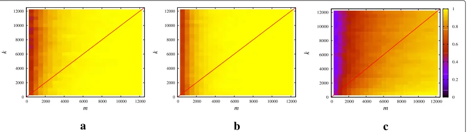
<5×10⁻²wherekis the estimated sparsity. In Fig. 1, we show results averaged over 1000 random instances, obtained by generating different sens-ing matrices from theγ-sparsified Gaussian ensemble. We underline that the values of the non-zero entries of the signals (which are drawn from a standard Gaussian distri-bution for this experiment) do not affect the performance in the noise-free case. Similarly, the lengthnof the signal plays no role in the estimation (see Proposition1).
The empirical probability of correct estimation is stud-ied as a function ofmandkfor three different regimes of parameterψ(k)defined in Remark2(see Fig.1) :
a) ψ(k)= 12(log(k)−log(logk)); b) ψ(k)=1;
c) ψ(k)=,3logk/k.
According to Theorem3(see also Remark2), whenm≥k, the relative error between the estimated sparsity and the true value of the sparsity degree tends to zero almost surely (i.e., with probability 1). This can be appreciated also in the numerical results in Fig.1, where the linem=k is drawn for simplicity. Moreover, we can see that for any fixedk, the error decreases whenmincreases.
6.2 Noisy measurements
In the second experiment, we show the performance of the EM-Sp algorithm when measurements are noisy according to the model proposed in (1) and we com-pare to the numerical sparsity estimator [20]. In order
a
b
c
Fig. 1Noise-free setting: empirical probability of success sparsity estimation as a function of sparsity degreekand number of measurements.
aψ(k)=12loglogkkbψ(k)=1cψ(k)= 3 "
2000 4000
6000
2000 4000 6000 0.025
0.05 0.1 0.19
MRE
EM-Sp Lopes
m
k
MRE
0.02 0.040.06 0.08 0.1 0.12 0.14 0.16 0.18 0.2
Fig. 2Experiment 2: MRE (in log-scale) of EM-Sp and Lopes’s estimator as a function of the sparsity degreekand the number of measurementsm, SNR=10 dB
to have a fair comparison, we perform this test on ternary signals in {−λ, 0,λ}n for which sparsity and numerical sparsity coincide. We then consider random sparse signals with non-zero entries uniformly chosen in {λ,−λ}, λ ∈ R, and SNR = λ2k/σ2 (see defini-tion in Secdefini-tion 3). Moreover, we set ψ(k) constant in order to focus on the effects of the additive noise in the estimation.
We remark that we compare only to [20] because, as illustrated in Section 1.1, the other proposed algo-rithms for sparsity degree estimation are based on signal reconstruction [14] (requiring a larger number of mea-surements and increased complexity, which would give
an unfair comparison) or are conceived for very specific applications [13,22].
In Fig. 2, we show the mean relative error (MRE) defined as
MRE=E
e
k,k
(41)
for different values of k and m in settings with
SNR = 10 dB and ψ(k) = 1/10. We appreciate that, in the considered framework, EM-Sp always outperforms the method based on the numerical sparsity estimation.
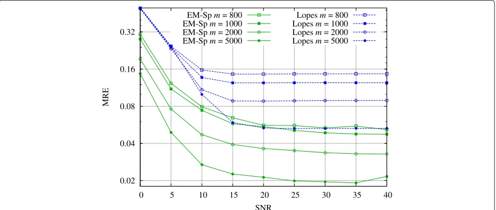
In Fig.3, we setk=1000,ψ(k)=1/3, and we vary the
SNRfrom 0 to 40 dB, whilem ∈ {800, 1000, 2000, 5000}.
0.02 0.04 0.08 0.16 0.32
0 5 10 15 20 25 30 35 40
MRE
SNR EM-Sp m = 800 EM-Sp m = 1000 EM-Sp m = 2000 EM-Sp m = 5000
Lopes m = 800 Lopes m = 1000 Lopes m = 2000 Lopes m = 5000
Again, we see that EM-Sp outperforms [20]. We spec-ify that a few tens of iterations are sufficient for the convergence of EM-Sp.
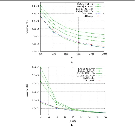
Finally, we compare the performance of EM-Sp with an oracle estimator designed as follows: we assume to know exactly the variancesα andβ and we generate measure-mentsyidistributed according to 2-GMM(1−p)φ(yi|α)+ pφ(yi|β), fori = 1,. . .,m; given the sequencey,α, and β, we then compute the ML estimate of p via EM. We name this estimator EM oracle. Comparing the estimates of p of EM-Sp and EM oracle, we can check if our 2-GMM approximation is reliable. We clearly expect that EM oracle performs better, as the measurements are really generated according to a 2-GMM, and also the true α
andβare exploited. However, our results show that the 2-GMM approximation is trustworthy. In Fig.4, we depict the sample variance of the estimatorpofp(obtained from 1000 runs) of EM-Sp and EM oracle. We show also the CR bound (see Section 5.3), which represents a perfor-mance lower bound for the estimation ofp. As explained in Section 5.3, the stochastic mean required in the CR bound for 2-GMM cannot be analytically computer and is here evaluated via Monte Carlo.
In both graphs of Fig. 4, we set k = 1000,m = k in Fig. 4a, andψ(k) = 1/10 in Fig.4b. We notice that in the considered regimes, EM oracle and CR bound are very close and not really affected by theSNR. Regarding EM-Sp, we observe that (a) keepingk,γ fixed, EM-Sp gets closer
a
b
to the optimum as theSNRincreases; and (b) keepingk,m fixed, we can find an optimalγ that allows us to get very close to the optimum.
6.3 Compressibility of real signals
In this section, we test our EM-Sp algorithm to eval-uate the compressibility of real signals. Specifically, we consider images which are approximately sparse in the discrete cosine transform (DCT) domain, that is, they are well represented by few DCT coefficients. Our aim is to estimate the number k of significant DCT coeffi-cients. More precisely, we seek the minimumksuch that the best-k approximationxk has a relative error smaller approximatelyτ, namelyxk−x22 ≤ τx22. Since DCT coefficients of natural images usually have a power-law decay of the formxi ≈ c/i, the following approximation holds
xk−x22
x22 ≈
-n
k x−2dx
-n 1 x−2dx
∝k−1 (42)
and since according to theoretical derivationγ ∝1/k, we fixγ ∝ τ. Tuningγ proportionally toτ allows to adapt better the sparsity of the sensing matrix to the expected signal sparsity: for largerτ’s, we expect smallerks, which call for largerγ to have the sufficient matrix density to pick the non-zero entries.
In the proposed experiments, we fix γ = cτ with c=5·10−2and we initializeπi(0)= 12for alli=1,. . .,m, while we setβandαrespectively as the signal energy and
the noise energy (namely, the error of the best-k
approxi-mation), evaluated from the measurements:β= y 2 2
m and α=τβ.
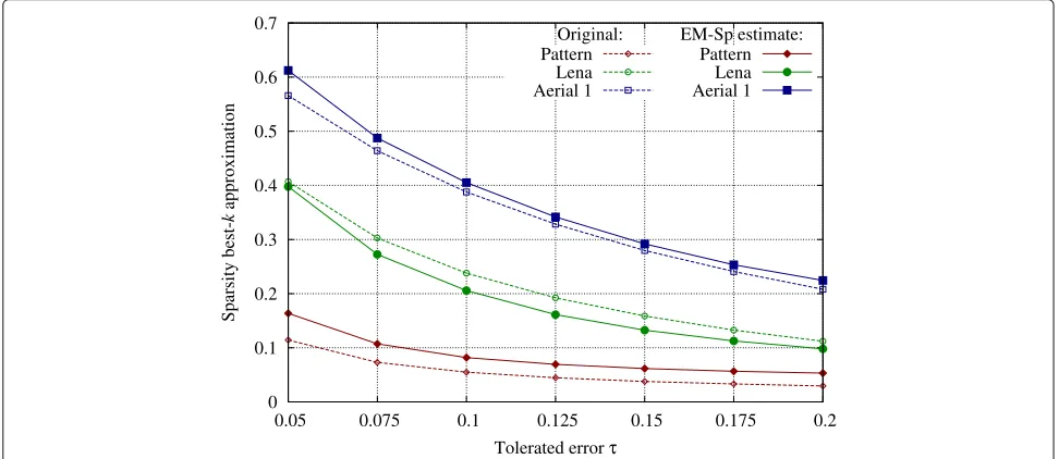
In Fig.5, we depict the results on threen = 256×256 images (shown in Fig.6) represented in the DCT basis (DCT is performed on 8×8 blocks). Specifically, we show original and estimated sparsity (they-axis represents the ratiok/n), averaged on 100 random sensing matrices. The images have been chosen with different compressibilities, to test our method in different settings. We appreciate that for all the images and across different values ofτ, we are able to estimatekwith a small error. This experiment shows then that EM-Sp can be practically used to estimate the compressibility of real signals.
6.4 Sparsity estimation for signal recovery
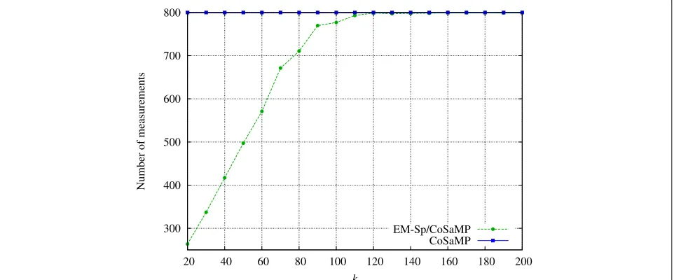
We have already remarked that the knowledge of the sparsity degree k is widely used for signal recovery in CS. In this section, we consider CoSaMP [9], an algo-rithm which can recover a sparse signal (exactly or with a bounded error, in the absence and in the presence of noise, respectively) if a sufficient number of measure-ments m is provided, and assuming the knowledge an upper bound kmax for k. Our aim is to show that EM-Sp can be used as a pre-processing for CoSaMP when kis not known; specifically, we estimate kto design the number of measurements necessary for CoSaMP recov-ery. Subsequently, we denote this joint procedure as EM-SP/CoSaMP.
We compare CoSaMP with EM-Sp/CoSaMP in the fol-lowing setting. We consider a familySof signals of length
0 0.1 0.2 0.3 0.4 0.5 0.6 0.7
0.05 0.075 0.1 0.125 0.15 0.175 0.2
Sparsity
best-k
approximation
Tolerated error τ
Original: EM-Sp estimate: Pattern
Lena Aerial 1
Pattern Lena Aerial 1
Fig. 5Experiment 3: compressibility of real signals, with non-exactly sparse representations. We estimateksuch thatxk−x22 x2
2 < τ
Fig. 6Non-exactly sparse signals: images with approximately sparse DCT representation: pattern, Lena, and aerial
n = 1600 and (unknown) sparsity k ∈ {20, 200} (then, kmax = 200). The value ofkand the position of the non-zero coefficients are generated uniformly at random, and the non-zero values are drawn from a standard Gaussian distribution. Since k is not known, the number of measurements needed by CoSaMP has to be dimensioned on kmax: assuming SNR = 30 dB, from the literature, we get that mC = 4kmax are sufficient to get a satisfactory recovery using dense Gaussian sensing matri-ces. In our specific setting, we always observe a mean relative error MRErec = x−x2/x2 < 5.5×10⁻² (for each k ∈ {20, 200}, 100 random runs have been performed).
We propose now the following procedure.
1 First sensing stage and sparsity estimation: we take mSmCmeasurements viaγ-sparsified matrix in
(2), and we provide an estimatekofk using Algorithm1.
2 Second sensing stage and recovery: we add a sufficient number of measurements (dimensioned overk) and then perform CoSaMP recovery.
Specifically, the following assessments have been proved to be suitable for our example:
• We estimatek with EM-Sp frommS= kmax2 sparsified measurements, withγ =6/kmax; • Since underestimates ofk are critical for CoSaMP,
we considerkequal to 2 times the estimate provided by EM-Sp;
• We addmA=4kGaussian measurements, and we run CoSaMP with the so-obtained sensing matrix withmS+mArows. WhenmS+mA>mC, we reduce the total number of measurements tomC.
300 400 500 600 700 800
20 40 60 80 100 120 140 160 180 200
Number of measurements
k
EM-Sp/CoSaMP CoSaMP
0 0.01 0.02 0.03 0.04 0.05 0.06 0.07 0.08
20 40 60 80 100 120 140 160 180 200
MRE
rec
k
EM-Sp/CoSaMP CoSaMP
Fig. 8The gain obtained by EM-Sp/CoSaMP in terms of measurements has no price in terms of accuracy: the recovery mean relative error is close to that of pure CoSaMP
We show the results averaged over 100 random experiments. In Fig. 7, we compare the number of measurements used for recovery, as a function of the sparsity degree k: a substantial gain is obtained in terms of measurements by EM-Sp/CoSaMP, with no significant accuracy loss. In Fig. 8, we can see that CoSaMP and EM-Sp/CoSaMP algorithms achieve similar MRErec.
7 Conclusions
In this paper, we have proposed an iterative algorithm for the estimation of the signal sparsity starting from compressive and noisy projections obtained via sparse random matrices. As a first theoretical contribution, we have demonstrated that the estimator is consistent in the noise-free setting and we characterized its asymptotic behavior for different regimes of the involved parameters, namely the sparsity degree k, the number of measure-mentsm, and the sensing matrix sparsity parameter γ. Then, we have showed that in the noisy setting, the pro-jections can be approximated using a 2-GMM, for which the EM algorithm provides an asymptotically optimal estimator.
Numerical results confirm that the 2-GMM approach is effective for different signal models and outperforms methods known in the literature, with no substantial increase of complexity. The proposed algorithm can rep-resent a useful tool in several applications, including the estimation of signal sparsity before reconstruction in a sequential acquisition framework, or the estima-tion of support overlap between correlated signals. An important property of the proposed method is that it does not rely on the knowledge of the actual sensing
matrix, but only on its sparsity parameter γ. This enables applications in which one is not interested in signal reconstruction, but only in embedding the spar-sity degree of the underlying signal in a more compact representation.
Endnote
1The code to reproduce the simulations proposed in
this section is available at https://github.com/sophie27/ sparsityestimation
Appendix
Proofs of results in Section 4 Proof of Proposition1
It should be noticed thatP(ωi =0)=(1−γ )θn, whereθ ∈ [0, 1] is the parameter to be optimized. Since the rows of the matrixAare independent, 5 so areωi, and considering that the eventωi = 0 is equivalent to the event that the support of ith row of Ais orthogonal to the support of signalx, the ML estimation computes
θo=argmax
θ∈[0,1] logf(ω
|θ)=m
i=1
f(ωi|θ) (43)
=argmax
θ∈[0,1] m
i=1
log1−(1−γ )θnωi(1−γ )θn(1−ωi)
(44)
from which
θo= log
1−ω0
m
nlog(1−γ ) . (45)
Proof of Theorem2
Let us consider ωi as defined in (15) and let pk = ω0
m where the index emphasizes the dependence on the sparsity degree. We thus have:
Pe(ko,k) > ing the Chernoff-Hoeffding theorem [38], the above tail probability is upper bounded as
Peko,k
> ≤2e−2mξk2 (56)
and we obtain the first part of the statement. Choosing
=
and from Borel-Cantelli Lemma [39], we conclude that
P
Proof of Theorem3 From Theorem2, we have
P.e
We have
a) Ifψ(k)→ ∞thenk =Oψ(k)−1; b) Ifψ(k)=(1)thenk =Og(k)−1/2; c) Ifψ(k)→0thenk=O(ψ(k)).
We conclude that in all three cases (a), (b), and (c) the thresholdkk−→→∞0.
Proof of Theorem4
Letk be defined as in (23). From Lemma2, we have, for
where the last inequality is obtained noticing that
m≥max
definitely. Since 2ρ > 1, from the Borel-Cantelli lemma, we deduce that
Proof of Theorem5
In this section, we prove Theorem5.
Lemma 1Let A be chosen from the γ-sparsified Gaussian ensemble uniformly at random and y be given in (14), pk=1−(1−γ )k, andω=1(Ax=0)then As already noticed throughout the paper, the measure-ment yi is a mixture of Gaussians with zero mean and variance depending on the overlap between the support of theith row ofAand supp(x). Suppose thatS ⊆ supp(x) is this overlap which happens with probability pS =
(1−γ )k−|S|γ|S|, then the variance of the Gaussian is given byαS= xS2
γ +σ2. Standard computations lead to
E Var(yi)|ωi=1= exactlyks−1−1possible sets of cardinalityscontaining, i.e., the number of selections of the remainings−1 objects among k − 1 positions. This observation and the fact x=0,∀ /∈supp(x)leads to
Var Var(yi)|ωi=1 (82)
Proof of Theorem5
Letψ(k) = γkand consider the sequence of probability density functions
and by the Lagrange Theorem [40], we obtain
g(t,α)=g(t,α)¯ +∂g that the first-order term in Taylor’s expansion of g(t;α) vanishes due to conditional mean result from Theorem2
Putting this expression into (87), we obtain
++
Through standard computations, we see that the
maxi-mizing value is obtained fort=
"
and using Lemma1, we conclude
Proof of Corollary1 From Theorem5, we have
++
2-GMM: Two-component Gaussian mixture model; CS: Compressed sensing; CoSaMP: Compressive sampling matching pursuit; DCT: Discrete cosine transform; EM: Expectation-maximization; ML: Maximum likelihood; MRE: Mean relative error; OMP: Orthogonal matching pursuit; SNR: Signal-to-noise ratio
Acknowledgments
The authors thank the European Research Council for the financial support for this research. We express our sincere gratitude to the reviewers for carefully reading the manuscript and for their valuable suggestions.
Funding
This work has received funding from the European Research Council under the European Community’s Seventh Framework Programme
(FP7/2007-2013)/ERC grant agreement no. 279848.
Availability of data and materials Please contact the corresponding author
([email protected]) for data requests.
Authors’ contributions
All the authors contributed equally, read, and approved the final manuscript.
Competing interests
The authors declare that they have no competing interests.
Publisher’s Note
Springer Nature remains neutral with regard to jurisdictional claims in published maps and institutional affiliations.
Author details
1National Research Council of Italy, IEIIT-CNR, c/o Politecnico di Torino, Corso
Duca degli Abruzzi 24, 10129 Torino, Italy.2Politecnico di Torino, DAUIN, Corso Duca degli Abruzzi 24, 10129 Torino, Italy.3Politecnico di Torino, DET, Corso Duca degli Abruzzi 24, 10129 Torino, Italy.
Received: 26 January 2018 Accepted: 19 August 2018
References
1. D.L. Donoho, Compressed sensing. IEEE Trans. Inf. Theory.52(4), 1289–1306 (2006)
2. E. Candes, T. Tao, Near optimal signal recovery from projection: universal encoding strategies?. IEEE Trans. Inf. Theory.52(12), 5406–5425 (2006) 3. F. Zeng, L. Chen, Z. Tian, Distributed compressive spectrum sensing in
cooperative multihop cognitive networks. IEEE J. Sel. Topics Signal Process.5(1), 37–48 (2011)
4. L. Gan, inIEEE Int. Conf. DSP. Block compressed sensing of natural images, (2007), pp. 403–406
5. E. Arias-Castro, E.J. Candes, M.A. Davenport, On the fundamental limits of adaptive sensing. IEEE Trans. Inf. Theory.59(1), 472–481 (2013) 6. M.A. Figueiredo, R.D. Nowak, S.J. Wright, Gradient projection for sparse
reconstruction: application to compressed sensing and other inverse problems. IEEE J. Sel. Topics Signal Process.1(4), 586–597 (2007)
7. A. Mousavi, A. Maleki, R.G. Baraniuk, Asymptotic analysis of LASSOs solution path with implications for approximate message passing (2013). preprint available at arXiv:1309.5979v1
8. J.A.A. Tropp, C. Gilbert, Signal recovery from random measurements via orthogonal matching pursuit. IEEE Trans. Inf. Theory.53, 4655–4666 (2007)
9. D. Needell, J.A. Tropp, CoSaMP: iterative signal recovery from incomplete and inaccurate samples. Appl. Comput. Harmonic Anal.26(3), 301–321 (2008)
10. D. Valsesia, S.M. Fosson, C. Ravazzi, T. Bianchi, E. Magli, in2016 IEEE International Conference on Multimedia Expo Workshops (ICMEW). Sparsehash: embedding jaccard coefficient between supports of signals, (2016), pp. 1–6
11. R. Ward, Compressed sensing with cross validation. IEEE Trans. Inf. Theory. 55(12), 5773–5782 (2009)
12. Y.C. Eldar, Generalized sure for exponential families: applications to regularization. IEEE Trans. Signal Process.57(2), 471–481 (2009) 13. SK Sharma, S Chatzinotas, B Ottersten, Compressive sparsity order
estimation for wideband cognitive radio receiver. IEEE Trans. Signal Process.62(19), 4984–4996 (2014)
14. Y. Wang, Z. Tian, C. Feng, Sparsity order estimation and its application in compressive spectrum sensing for cognitive radios. IEEE Trans. Wireless Commun.11(6), 2116–2125 (2012)
15. D.M. Malioutov, S. Sanghavi, A.S. Willsky, inProc. IEEE Int. Conf. Acoust. Speech Signal Process. (ICASSP). Compressed sensing with sequential observations, (2008), pp. 3357–3360
16. M.S. Asif, J. Romberg, inSignals, Systems and Computers, 2008 42nd Asilomar Conference On. Streaming measurements in compressive sensing:1filtering, (2008), pp. 1051–1058
17. P.J. Garrigues, L. El Ghaoui, inNeural Information Processing Systems (NIPS). An homotopy algorithm for the Lasso with online observations, vol. 21, (2008)
18. Y. You, J. Jin, W. Duan, N. Liu, Y. Gu, J. Yang, Zero-point attracting projection algorithm for sequential compressive sensing. IEICE Electron. Express.9(4), 314–319 (2012)
19. T.V. Nguyen, T.Q.S. Quek, H. Shin, Joint channel identification and estimation in wireless network: sparsity and optimization. IEEE Trans. Wireless Commun.17(5), 3141–3153 (2018)
20. M.E. Lopes, inProc. 30th Int. Conf. Machine Learning. Estimating unknown sparsity in compressed sensing, vol. 28 (Proceedings of Machine Learning Research, Atlanta, 2013)
21. M.E. Lopes, Unknown sparsity in compressed sensing: denoising and inference. IEEE Trans. Inf. Theory.62(9), 5145–5166 (2016)
22. S. Lan, Q. Zhang, X. Zhang, Z. Guo, inIEEE Int. Symp. on Circuits and Systems (ISCAS). Sparsity estimation in image compressive sensing, (2012) 23. A. Agarwal, L. Flodin, A. Mazumdar, inIEEE International Symposium on
Information Theory (ISIT). Estimation of sparsity via simple measurements, (2017), pp. 456–460
24. Z. Bar-Yossef, T.S. Jayram, R. Kumar, D. Sivakumar, L. Trevisan, ed. by J.D.P. Rolim, S. Vadhan. Randomization and Approximation Techniques in Computer Science (RANDOM) (Springer, Berlin, 2002), pp. 1–10 25. P.B. Gibbons, ed. by M. Garofalakis, J. Gehrke, and R. Rastogi. Data Stream
Management: Processing High-Speed Data Streams (Springer, Berlin, 2016), pp. 121–147
26. V. Bioglio, T. Bianchi, E. Magli, inProc. IEEE Int. Conf. Acoust. Speech Signal Process. (ICASSP). On the fly estimation of the sparsity degree in compressed sensing using sparse sensing matrices, (2015), pp. 3801–3805
27. W. Wang, M.J. Wainwright, K. Ramchandran, Information-theoretic limits on sparse signal recovery: dense versus sparse measurement matrices. IEEE Trans. Inf. Theory.56(6), 2967–2979 (2010)
28. D. Omidiran, M.J. Wainwright, High-dimensional variable selection with sparse random projections: measurement sparsity and statistical efficiency. JMLR.11, 2361–2386 (2010)
29. C. Ravazzi, S.M. Fosson, T. Bianchi, E. Magli, in2016 IEEE International Conference on Acoustics, Speech and Signal Processing (ICASSP). Signal sparsity estimation from compressive noisy projections viaγ-sparsified random matrices, (2016), pp. 4029–4033
31. D. Omidiran, M.J. Wainwright, High-dimensional variable selection with sparse random projections: measurement sparsity and statistical efficiency. J. Mach. Learn. Res.11, 2361–2386 (2010)
32. R. Berinde, P. Indyk, M. Ruzic, inCommunication, Control, and Computing, 2008 46th Annual Allerton Conference On. Practical near-optimal sparse recovery in the l1 norm, (2008), pp. 198–205
33. A. Gilbert, P. Indyk, Sparse recovery using sparse matrices. Proc. IEEE. 98(6), 937–947 (2010)
34. P. Li, C-H Zhang, inProceedings of the 18th International Conference on Artificial Intelligence and Statistics (AISTATS) 2015. Compressed sensing with very sparse gaussian random projections, (2006), pp. 617–625 35. E.J. Candès,The restricted isometry property and its implications for
compressed sensing. (Compte Rendus de l’Academie des Sciences, Paris, France). ser. I346, 589–592 (2008)
36. M.A.T. Figueiredo, A.K. Jain, Unsupervised learning of finite mixture models. IEEE Trans. Pattern Anal. Mach. Intell.24, 381–396 (2000) 37. C.F.J. Wu, On the convergence properties of the em algorithm. Ann.
Statist.11(1), 95–103 (1983)
38. W. Hoeffding, Probability inequalities for sums of bounded random variables. J. Am. Stat. Assoc.58(301), 13–30 (1963)
39. W. Feller,An introduction to probability theory and its applications, vol. 1. Wiley, New York, 1968)