Int. J. Data Envelopment Analysis (ISSN 2345-458X)
Vol.5, No.2, Year 2017 Article ID IJDEA-00422, 20 pages Research Article
Efficiency Analysis in Multi-Stage Network
DEA-R Models
M.R. Mozaffaria*, M.Saneib, J. Jablonskyc
(a) Department of Mathematics, Islamic Azad University, Shiraz Branch, Shiraz, Iran.
(b) Department of Mathematics, Islamic Azad University, Central Tehran Branch, Tehran, Iran.
(c) Department of Econometrics, University of Economics, Prague, Czech Republic
Received November 20, 2016, Accepted February 22, 2017
Abstract
In many organizations and financial institutions, it is in many cases more cost and time efficient to access ratio data. Therefore, it is of great importance to evaluate the performance of decision-making units (DMUs) which only have access to ratios of inputs to outputs or vice versa (for instance, ratio of employees to students, ratio of assets to liabilities and ratio of doctors to patients). In this paper, we will propose two-stage network DEA-R model with multi-objective linear programming (MOLP) structures. Then, introducing a production possibility set (PPS) in each network stage, we will compare efficiency values in network DEA and DEA-R. In the end, through an applied study on 22 medical centers which treat special patients in three stages, we will suggest an output-oriented multi-stage network DEA-R model under assumption of CRS technology. The medical centers are evaluated in all three stages based on overall network efficiency. The results of the analysis are presented and a future research in this field is discussed in the final section of the paper.
Keywords: DEA, Network DEA, DEA-R models, efficiency.
1. Introduction
Data envelopment analysis (DEA) is a non-parametric method for evaluating performance of a set of decision-making units (DMUs). Measuring efficiency, as an important factor in evaluation of a company or organization’s performance, has always been a topic of interest among researchers. In 1957, Farrell proposed the idea of an efficient piecewise linear frontier as an alternative to estimating production function. However, there was an apparent issue with the number of inputs and outputs in the DMUs (Farrell, 1957). Charnes et al. (1978) extended Farrell’s non-parametric method for a multiple inputs and outputs system through mathematical programming. Their model came to be known as CCR models. Later on, several articles and models were presented in this area, out of which we can mention the infamous BCC model introduced by Banker et al. (1984) for variable returns to scale (VRS) production technology.
Further developing the cone-ratio DEA model, Fare and Grosskopf (1996, 2000) presented network DEA models. Chen et al. (2006) introduced the DEA game model for measuring efficiency in supply chains. Kao and Hwang (2008) studied efficiency decomposition in two-stage processes for 24 non-life insurance companies in Taiwan. Their model is one of the most known two-stage DEA network models at all. Combining game approach with efficiency decomposition in two-stage DEA models, Liang et al. (2008) evaluated 30 commercial banks using centralized and non-cooperative models. Chen et al. (2009) studied the subject of additive efficiency in two-stage DEA under both constant and variable returns to scale assumptions (CRS / VRS) and rated the DMUs based on the results. Kao (2009) extended his previous paper and evaluated efficiency decomposition in network DEA for parallel and series systems using the same case (24
insurance companies in Taiwan). Cook et al. (2010) presented three-stage and multi-stage network DEA models with parallel processes based on additive efficiency decomposition. Chen and Yan (2011) introduced three network DEA models for evaluating performance of supply chain while considering internal resource waste. They proposed production possibility sets for supply chain based on centralized, decentralized and mixed mechanisms.
Chen et al. (2012) studied a new methodology for performance evaluation through two-stage network DEA in order to evaluate environmental conditions among 23 companies. Li et al. (2012) presented DEA models for extended two-stage network structures with additional inputs in 3 regions in China. One of the advantages of their work was an extension of the model introduced in (Liang et al., 2008).
Guo et al. (2016) obtained overall efficiency by selecting suitable weights and applying them to a multi-objective programming problem within the framework of network DEA for two-stage.
One of the first ratio DEA models (DEA-R) was introduced in (Despic et al., 2007). The authors extended the subjects of arithmetic, geometric and harmonic efficiency to DEA, DEA-R and multiplicative models based on the relationships between arithmetic, geometric and harmonic means. Furthermore, they revealed the efficiency value in input-oriented DEA-R to be greater than or equal to efficiency value in DEA. Studying 21 medical centers, Wei et al. (2011a) proposed the subject of pseudo-inefficiency in DEA. In another study (Wei et al., 2011b), they evaluated the relationship between CCR models in DEA and DEA-R through comparing optimal weights in DEA and DEA-R. Wei et al. (2011c) presented output-oriented DEA-R models with weight restrictions and made a comparison between them and DEA-R models with harmonic. Liu et al. (2011) suggested DEA models without explicit inputs; they proposed the subject of ratio data and corresponding production possibility sets (PPS) under general conditions. Mozaffari et al. (2014a) analyzed the relationship between DEA models without explicit inputs and DEA-R models. A cost and revenue efficiency in DEA and DEA-R models is studied in (Mozaffari et al., 2014b). Olesen et al. (2015) proposed the subject of efficiency analysis based on ratio measure. They did a detailed study on production possibility set and dependence of inputs and outputs on ratio data under constant and variable returns to scale technology assumptions. This article differs from their study in terms of dependence of inputs and outputs - ratio
data are available in this study and they are defined as independent.
The rest of the paper is organized as follows. In Section 2, two-stage DEA models and basic concepts of DEA-R are introduced. Section 3 presents output-oriented multi-stage DEA-R models along with their production possibility sets (PPS). A three-stage DEA-R model is formulated in Section 4. A case study that demonstrates and compares stage efficiencies and overall efficiencies using the structure of multiple objective linear programming is presented in Section 5. Final section of the paper contains conclusions and suggestions for future research.
2. Theoretical background
In this section, selected two-stage serial DEA models are formulated to the extent necessary for further analysis, and basic ideas of DEA-R models are presented. 2.1 Two-stage DEA models
Let us consider a two-stage structure, where in the first stage, m inputs
XJ x1j,...,xmj
produce b outputs
ZJ z1j,...,zbj
. In the second stage, theoutputs
ZJ
z1j,...,zbj
are turned into inputs, which in turn produce s final outputs
YJ
y1j,...,ysj
. The inputs,intermediate characteristics and the final outputs of the j-th DMU are Xj = (x1j,…, xmj), Zj = (z1j,…, zbj), and Yj = (y1j,…, ysj) respectively. A model for evaluation of the DMUo in the first stage based on the idea presented in (Despotis et al., 2016) is introduced as follows:
Minimize
f o f b
f io i m
i
z x e
1 =
1 = 1
Subject to 0
1 = 1
=
f f jb
f ij i m
i
z
x
0
1 = 1 =
r rjb r fj f b f
y
z
j 1,...,n0 ; 0 ;
0
f r
i
v
s r b f mi1,..., ; 1,..., ; 1,...,
A model that evaluates the efficiency of the DMUo in second stage is formulated in a similar way:
Minimize 2 =1
=1 b f fo f b r ro r z e y
Subject to
0
1 = 1 =
f fjb f ij i m i
z
x
nj1,..., (2)
0
1 = 1 =
r rjb r fj f b f
y
z
j 1,...,n0 ; 0 ;
0
f r
i
v
s r b f mi1,..., ; 1,..., ; 1,...,
Both models (1) and (2) have the same set of constraints. The weights
i,
f andr
are assigned to inputs, intermediate characteristics and final outputs respectively. They are variables of models (1) and (2). Symbolse
1 ande
2 stand for efficiency scores in stages one and two, respectively. Based on the efficiency decomposition approach, overall efficiency is defined as the weighted average of stage efficiencies:
21
0
e
1
e
e
,1
0
(3) The following model is solved in order to obtain the overall efficiency score (3):Minimize =1 =1
=1 =1
,
b m f fo i io f i b sf fo r ro
f r
z
x
h
z
y
Subject to
0
1 = 1 =
f fjb f ij i m i
z
x
n
j
1
,...,
(4)0
1 = 1 =
r rjs r fj f b f
y
z
j
1
,...,
n
0 ; 0 ;
0
f r
i
v
s r b f mi1,..., ; 1,..., ; 1,...,
Model (4) is a bi-objective fractional programming problem. It can be solved using various multiple objective techniques - weighted sum of particular objective functions, lexicographic approach, or bi-level method.
2.2 Basic concepts of DEA-R models In this section, we present the relationship between DEA and DEA-R models under the assumption of constant returns to scale technology based on the ideas of Despic et al. (2007). Let us suppose the following formulation of DEA-R model: Maximize
u
,
v
s r ro rj r m i io ij i j oy
y
u
x
x
v
e
1 1min
Subject to
1
1 =
r s ru
(5)1
1 =
i m iv
0
;
0
i rv
Of course the assumption of positive data is essential and all ratios
io ij x x and ro rj y y
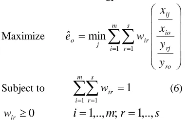
must be defined. Despic et al. (2007) presented their DEA-R efficiency model for evaluation of DMUo in constant returns to scale technology as follows:
Maximize
m i s r ro rj io ij ir j oy
y
x
x
w
e
1 1min
ˆ
Subject to
1
1 1
s r ir m iw
(6)0
ir
w
i
1
,..,
m
;
r
1
,..,
s
Where wir is the weight of the ratio in the objective function (6).
Wei et al. (2011a) proved the relationship between models (5) and (6) as eo eˆo.
3. Two-stage network DEA-R models Evaluating DMUs which possess ratio data such as
j j
X Z and
j j
Z
Y requires models
which firstly, possess the requirements of the respective production possibility set, and secondly, are able to calculate efficiency value of the units. In this section, we first suggest two-stage DEA-R models and then introduce the production possibility set in each stage. In the second part, we will propose two-stage DEA-R models using MOLP and present numerical expressions in the end. (Fig 1)
3.1 Efficiency in two-stage DEA-R model
Assume that we have (Xj,Zj,Yj) for DMUj where
j j X Z and j j Z
Y ratios are
available. Our aim is to evaluate the DMUs in a two-stage process using the defined ratios. Our proposed output-oriented CRS model for the first stage is as follows:
Minimize
E
1
1Subject to 1
1 1 =
b f io fo ij fj if m ix
z
x
z
w
nj1,..., (7)
1
1 1
b f if m iw
, 0 ifw
i
1
,..,
m
;
f
1
,..,
b
.The output-oriented DEA-R envelopment model for evaluation of the DMUo can be The output-oriented DEA-R envelopment model for evaluation of the DMUo can be formulated as follows:
Maximize
1Subject to 1 1
1 n
j o
j
j j o
Z Z X X
(8)1 1
1
1,
0,
1,..., .
n j j j
j
n
Definition 1. DMUo is DEA-R efficient (output-oriented DEA-R efficient) if and only if the optimal objective function value of model (8)
*1
1
.In the second stage, our proposed output-oriented DEA-R model is as follows: Minimize
E
2
2Subject to. 2
1 1 =
b f fo ro fj rj if s r z y z y w nj 1,..., (9)
1
1 1
b f rf s rv
0
rfv
r
1
,..,
s
;
f
1
,..,
b
The output-oriented envelopment model under CRS technology in stage 2 for evaluation of DMUo can be written as follows:
Maximize
2 Subject to 22 1
n
j o
j
j j o
Y Y Z Z
2 1 21,
0,
1,..., .
n
j j
j
j
n
(10)Definition 2. DMUo is DEA-R efficient (output-oriented DEA-R efficient) if and only if the optimal objective function value of model (10)
*2
1
.3.2 Two-stage Network DEA-R models based on MOLP
In this section, we will propose two-stage network DEA models which use MOLP. First, a bi-objective linear programming model is suggested for measuring overall efficiency of DMUO with ratio data
defined as j j X Z and
j j Z
Y (CRS,
output-oriented), And finally, the bi-objective linear programming model is solved using the lexicographic and adaptive weighted sum approaches. Combining the restrictions of models (7) and (9), we suggest the bi-objective linear model (11) for measuring overall efficiency of the two-stage DEA-R process. Model (11) is proposed for output-oriented evaluation of DMUo under the assumption of constant returns to scale technology based on MOLP.
Minimize
1,
2
Subject to.
m i b f io fo ij fj ifx
z
x
z
w
1 1 1
nj1,..., (11)
s r b f fo ro fj rj rfz
y
z
y
v
1 1 2
j1,...,n1 1 1 =
b f rf s rv 1
1 1 =
b f if m i w 0 ; 0 if rf w v m i b f sr 1,..., ; 1,..., ; 1,...,
The second step, the set of constraints is extended by 1 = 1* and the second objective function is optimized. Using this approach a Pareto efficient solution of the MOLP problem (11) is given. We propose an envelopment model for evaluating the overall efficiency of a two-stage network DEA-R as follows:
Maximize
1
2
Subject to 1 1 1
n
j o
j
j j o
Z Z
X X
2
2 1
n
j o
j
j j o
Y Y
Z Z
(12)1 2
1 2
1 1
1 2
,
,
0,
0,
1,..., .
n n
j j
j j
j j
P
P
j
n
Model (12) is a linear programming problem, in which
p
1 andp
2 are parameters determining overall efficiency of the two-stage process. The variable
1j and
2j correspond to stage 1 and stage 2respectively. If 2 0 1
j n
j
then only stage
1 process is considered. Similarly, if
0 1 1
j
n
j
, then we consider the process in stage 2 only. However, if we consider
1 1 1
p
j n
j
and 2 2
1
p
j n
j
, where p1+p2=1,
p1, p2 > 0, the Pareto optimal solution of model (11) defines the overall efficiency of DMUo of the two-stage models with ratio data.
3.3 Illustration
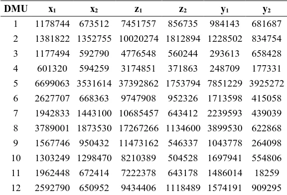
The illustration presented in this section is given from (Kao and Hwang, 2008) where 24 non-life insurance companies have been analyzed. Despotis et al. (2016) and Guo et al. (2016) have previously used this data set in order to measure efficiency of two-stage processes and overall efficiency. We will use the same data set in order to evaluate the two-stage DEA-R process using presented MOLP techniques. The original data set is presented in Table 1.
Table 1. Inputs, intermediate variables, and outputs of 24 DMUs
DMU x1 x2 z1 z2 y1 y2
13 2609941 1368802 13921464 811343 3609236 223047 14 1396002 988888 7396396 465509 1401200 332283 15 2184944 651063 10422297 749893 3355197 555482 16 1211716 415071 5606013 402881 854054 197947 17 1453797 1085019 7695461 342489 3144484 371984 18 757515 547997 3631484 995620 692731 163927 19 159422 182338 1141951 483291 519121 46857 20 145442 53518 316829 131920 355624 26537 21 84171 26224 225888 40542 51950 6491 22 15993 10502 52063 14574 82141 4181 23 54693 28408 245910 49864 0.1 18980 24 163297 235094 476419 644816 142370 16976
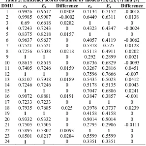
Table 2. Efficiency scores obtained by models (1), (2), (7) and (9) DMU e1 E1 Difference e2 E2 Difference
1 0.9926 0.9617 0.0309 0.7134 0.7152 -0.0018 2 0.9985 0.9987 -0.0002 0.6449 0.6311 0.0138 3 0.69 0.6618 0.0282 1 1 0 4 0.7243 0.7243 0 0.4323 0.4347 -0.0024 5 0.8375 0.8218 0.0157 1 1 0 6 0.9637 0.9637 0 0.4057 0.4119 -0.0062 7 0.7521 0.7521 0 0.5378 0.525 0.0128 8 0.7256 0.7038 0.0218 0.5113 0.4911 0.0202 9 1 1 0 0.292 0.2899 0.0021 10 0.8615 0.8615 0 0.6736 0.6829 -0.0093 11 0.7405 0.7246 0.0159 0.3267 0.2816 0.0451 12 1 1 0 0.7596 0.7666 -0.007 13 0.8107 0.7918 0.0189 0.5435 0.5023 0.0412 14 0.7246 0.7246 0 0.5178 0.5135 0.0043 15 1 1 0 0.7047 0.6806 0.0241 16 0.9072 0.8881 0.0191 0.3847 0.3857 -0.001
17 0.7233 0.7233 0 1 1 0
18 0.7935 0.7685 0.025 0.3976 0.3737 0.0239
19 1 1 0 0.4158 0.4158 0
20 0.9332 0.9332 0 0.9014 0.9014 0 21 0.7505 0.7505 0 0.2795 0.2906 -0.0111 22 0.5895 0.5802 0.0093 1 1 0 23 0.8501 0.8217 0.0284 0.5599 0.5599 0
24 1 1 0 0.3351 0.3351 0
This example consists of two inputs (x1, x2), two intermediate measures (z1, z2) and two outputs (y1, y2).
All ratios
1 1 x z ,
2 1 x z ,
1 2
x z
,
2 2
x z
,
1 1
z y
,
2 1
z y
,
1 2 z y ,
2 2 z
y are known. That is why we can
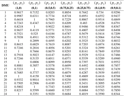
Table 3. Results obtained by MOLP models (11) and (12) with different parameters
DMU
(
p
1,
p
2)
(
p
1,
p
2)
(
p
1,
p
2)
(
p
1,
p
2)
(
p
1,
p
2)
(
p
1,
p
2)
(
p
1,
p
2)
(1,0) (0,1) (0.5,0.5) (0.75,0.25) (0.25,0.75) (0.1,0.9) (0.9,0.1)1 0.9617 0.7152 0.8203 0.8854 0.7642 0.734 0.9296 2 0.9987 0.6311 0.7734 0.8718 0.6951 0.6552 0.9437 3 0.6618 1 0.7965 0.7229 0.8867 0.9514 0.6849 4 0.7243 0.4347 0.5433 0.6209 0.483 0.4528 0.6791 5 0.8218 1 0.9022 0.8601 0.9486 0.9788 0.8367 6 0.9637 0.4119 0.5771 0.7219 0.4807 0.4369 0.8498 7 0.7521 0.525 0.6184 0.6787 0.5679 0.5414 0.7209 8 0.7038 0.4911 0.5785 0.6351 0.5312 0.5064 0.6746 9 1 0.2899 0.4495 0.6202 0.3525 0.3120 0.8032 10 0.8615 0.6829 0.7619 0.8087 0.7203 0.6974 0.8396 11 0.7246 0.2816 0.4056 0.5201 0.3324 0.2999 0.6261 12 1 0.7666 0.8679 0.9293 0.8141 0.7849 0.9705 13 0.7918 0.5023 0.6147 0.6921 0.5529 0.5214 0.7486 14 0.7246 0.5135 0.6011 0.6571 0.5539 0.5289 0.6960 15 1 0.6806 0.8099 0.8950 0.7397 0.7031 0.9552 16 0.8881 0.3857 0.5378 0.6699 0.4492 0.4088 0.7857 17 0.7233 1 0.8394 0.7771 0.9127 0.9632 0.7439 18 0.7685 0.3737 0.5028 0.6079 0.4287 0.3939 0.6951 19 1 0.4158 0.5874 0.7400 0.4869 0.4416 0.8768 20 0.9332 0.9014 0.9170 0.9250 0.9091 0.9045 0.9299 21 0.7505 0.2906 0.4189 0.5377 0.3431 0.3095 0.6479 22 0.5802 1 0.7343 0.6482 0.8468 0.9325 0.6056 23 0.8217 0.5599 0.6660 0.7357 0.6084 0.5783 0.7850 24 1 0.3351 0.5020 0.6684 0.4019 0.3590 0.8344
The second and third column of Table 2 presents the efficiency score obtained by models (1) and (7), i.e. models measuring the efficiency in the first stage of the production process using the output-oriented DEA model (1) and DEA-R model under CRS technology (7) respectively. There is a very small difference between efficiency values of the first stage in DEA and DEA-R – in many cases the efficiency scores are identical. The units 9, 12, 15, 19 and 24 are efficient at this stage. The last two columns of Table 2 present similar results for the second stage of the production process. They are calculated using models (2) and (9). The units 3, 5, 17 and 22 are efficient in the second stage measuring by both models.
Table 3 contains the results obtained by MOLP models (11) and (12). The
allows to decision makers analyzing the two-stage production process in more detail.
4. Three-stage network DEA-R processes
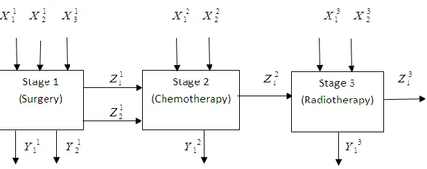
This section presents a three-stage network production process with inputs X1, X2 and X3, and final outputs Y1, Y2 and Y3 for all three stages. Z1 are intermediate measures - the outputs of the first stage and the inputs of the second stage. Z2 are the outputs of the second stage entering the third stage as its inputs. Z3 are the outputs of the third stage.
We propose a model for evaluation three-stage network DEA-R processes under the following assumptions:
a. The proposed model is output-oriented DEA-R envelopment model under the assumption of CRS technology.
b. Our proposed model is a parametric linear model in a three-stage network process; this model aims to increase the outputs in every stage in order to evaluate units with ratio data.
In all network stages, we consider the constraint ∑𝑛𝑗=1𝜆𝑗𝑡 = 𝑃𝑡 corresponding to
each stage 𝑡, on the condition that
𝑃1+𝑃2+𝑃3= 1. Therefore, since 𝜆𝑗𝑡≥ 0,
if ∑𝑛𝑗=1𝜆𝑗𝑡 = 0, then 𝜆𝑗𝑡 = 0 for every 𝑗.
In general, we consider two scenarios for the parameters 𝑃𝑡:
i) If 𝑃𝑡 ∈ {0,1} and 𝑃1+𝑃2+𝑃3 = 1, then
the proposed model can calculate the efficiency of every stage.
ii) If 𝑃𝑡∈ [0,1] and 𝑃1+𝑃2+𝑃3= 1, then
the proposed model can calculate the overall efficiency of our network.
c. Let I1, I2 and I3 are the sets of indices of inputs in all three stages. Similarly F1, F2 and F3, and R1, R2 and R3 are the sets of indices of intermediate measures and final outputs respectively.
d. In the suggested model, parameters 𝑃1, 𝑃2 and 𝑃3 correspond to variables 𝜆𝑗1, 𝜆𝑗2
and 𝜆𝑗3, respectively. Now, since the three stages of our network as well correspond
to 𝜆𝑗1, 𝜆𝑗2 and 𝜆𝑗3, therefore the parameters
𝑃1, 𝑃2 and 𝑃3 have a very significant role
in calculation of stage and overall efficiencies.
e. Variables
1j,
2j,
3j correspond to stages 1, 2 and 3, respectively.f. Since the three-stage network process is output-oriented, the proposed model aims to increase the output-to-input ratios, which are increased radially. Variables
𝜑1, 𝜑2 and 𝜑3 are used to increase the
outputs in stages one, two and three of a network with ratio data, respectively. The DEA-R model we propose for overall evaluation of three-stage serial production process is as follows:
Maximize
1
2
3
Subject to 1 1 1 1 1 1 1 n fj fo jj ij io
z
z
x
x
1 1;
f
F
I
i
(13) 1 1 1 1 1 1 1 n rj ro j
j ij io
y
y
x
x
i
I
1;
r
R
1 2 2 2 2 2 2 1 n lj lo jj ij io
z
z
x
x
i
I
1;
l
F
1 2 2 2 2 2 2 1 n rj ro j
j ij io
y
y
x
x
i
I
2;
r
R
2 3 3 3 3 3 3 1 n tj to j
j ij io
z
z
x
x
i
I
3;
t
F
3 3 3 3 3 3 3 1 n rj ro j
j ij io
y
y
x
x
iI3;rR3 3 3 3 3 3 3 1 n rj ro j
j tj to
y
y
z
z
i
I
3;
t
F
3
n j fo lo fj lj j z z z z 1 1 2 1 2 2
f
F
1;
l
F
2
n j lo to lj tj j z z z z 1 2 3 2 3 3
n
j lo
ro
lj rj j
z y z
y
1
2 3 2
3 3
rR3;lF2
n
j
j
p
1
1 1
,
n
j
j
p
1
2 2
,
n
j
j
p
1
3 3
p1 + p2 + p3 = 1,
0 ; 0 ;
0 2 3
1
j j
j
j1,...,n.Model (13) is a linear programming problem, in which
p
1,p
2 andp
3 are parameters determining overall efficiency for three-stage network processes. Generally speaking, model (13) can be a suitable alternative for model (8) in stage one and model (10) in stage two; in this regard, if we consider 𝑃1= 1 and 𝑃2= 𝑃3= 0, we can only calculate theefficiency of stage one, as ∑ 𝜆𝑗1= 1 and
∑ 𝜆𝑗2= ∑ 𝜆
𝑗3= 0. Similarly, we can
calculate the efficiency of later stages by changing the parameters 𝑃1, 𝑃2 and 𝑃3 to
zeros or ones. However, if the parameters
𝑃1, 𝑃2 and 𝑃3 were strictly greater than
zero, then all constraints used in each network stage would influence the overall efficiency.
5. A case study
Let us consider 22 Iranian medical centers
which provide necessary services to special patients with tumors. The data set available is taken from summer months 2016. The treatment process of patients with cancer diseases can generally be divided into three stages:
Stage 1 includes patients needing surgery.
Patients at this stage generally have special diseases and their tumors are either benign of types A or B, or they are malignant. All three groups of patients need surgery according to conclusions by an expert physician.
Stage 2 includes patients who need
chemotherapy based on doctor’s orders. This group generally consists of patients with special diseases who either have had a surgery in previous years and currently need chemotherapy, or did not undergo the surgery because of their age or other specific factors and now chemotherapy is needed.
Stage 3 includes radiotherapy. Generally,
this group of patients either has undergone surgery, chemotherapy and radiotherapy during past years and according to doctor’s diagnosis need radiotherapy, or has finished the treatment process and need radiotherapy in order to destroy the cancer cells after surgery or chemotherapy.
Generally, in treatment of patients with tumors, medical centers provide the following treatment processes after the radiology and sampling stages.
i) If the tumor was malignant, the stages of surgery, chemotherapy and radiotherapy are indeed essential.
ii) If the tumor was malignant but the patient was not able to undergo surgery due to age limits, chemotherapy and radiotherapy are performed.
iii) If the tumor was benign, there could only be a need for surgery based on doctor’s diagnosis.
The treatment process is graphically illustrated on Figure 2. It is three-stage process where the following input, intermediate and output variables are used:
1 1
x the number of patients with type A benign tumors needing a surgery,
1 2
x the number of patients with type B benign tumors needing a surgery,.
1 3
x
the number of patients with malignant tumors needing a surgery.1 1
y patients who only require surgery according to the doctor’s diagnosis and their surgery is only successful in the first stage; based on the post-surgery pathology report, these patients don’t need to continue treatment and only make annual visits to the physician for follow-ups.
1 2
y : Patients who undergo surgery, but cannot continue the treatment process due to age limits. Meaning the patients are not in a suitable condition to continue treatment after surgery and it is in their best interest to stop the process.
1 1
z : Number of special patients who have benign tumors, but for whom the need for chemotherapy becomes apparent in the radiological tests at the start of surgery.
1 2
z : Number of patients with malignant tumors who need chemotherapy following surgery.
2 1
x : Number of special patients who start the treatment process with chemotherapy because of their age or problems with other diseases such as heart or liver disease.
2 2
x : Number of patients who have had surgery in previous years and their respective physician has prescribed chemotherapy in the current annual screening.
2 1
y
: Number of special patients who have finished chemotherapy but don’t need radiotherapy because of special conditions or other diseases.2 1
z : Number of patients who have undergone chemotherapy in stage 2 and do not require radiotherapy
3 1
x : Number of patients who have undergone chemo and radiotherapy in previous years but currently require further radiotherapy based on doctor’s orders.
3 2
x : Number of patients who only need radiotherapy based on their tumor type and age.
3 1
z : Number of patients who recover following radiotherapy (relatively satisfied with treatment).
3 1
y : Number of patients who recover after undergoing all treatment stages (completely satisfied with treatment). Regarding patients visiting the 22 medical centers, due to the special conditions of patients and uncertainty of the treatment process in each stage (since there is a chance of cell proliferation and dependency of patient’s immune system), it’s often impossible to obtain accurate data in terms of inputs and outputs for each stage. Consequently, we usually only have access to a ratio of
1 1 ij
fj
x
z
,
1 1 ij rj
x
y
,
2 2 ij lj
x
z
and
3 3
ij tj
x z
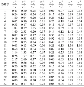
Table 4. Data related to the 22 Iranian medical centers in summer 2016 (stage 1)
DMU
1 1 1 1 z x
1 2 1 1 z x
1 1 1 2 z x
1 2 1 2
z x
1 1 1 3 z x
1 2 1 3
z x
1 1 1 1 y x
1 1 1 2 y x
1 1 1 3 y x
1 2 1 1 y x
1 2 1 2
y x
1 2 1 3
y x
1 0.10 0.14 0.15 0.22 0.43 0.61 0.93 1.40 4.00 0.58 0.88 2.50 2 0.22 0.06 0.08 0.02 1.56 0.44 0.72 0.25 5.00 1.07 0.37 7.41 3 0.01 0.51 0.01 0.30 0.02 0.66 0.98 0.59 1.27 1.66 1.00 2.16 4 0.38 0.07 0.50 0.09 1.88 0.34 0.81 1.08 4.06 0.39 0.52 1.96 5 0.10 0.19 0.04 0.07 0.27 0.52 0.73 0.29 2.03 2.26 0.89 6.24 6 0.17 0.23 0.19 0.26 0.56 0.76 0.70 0.81 2.36 0.62 0.71 2.08 7 0.12 0.07 0.06 0.04 0.05 0.03 0.93 0.48 0.42 1.88 0.98 0.85 8 0.43 0.22 0.48 0.25 1.00 0.51 0.57 0.64 1.34 0.72 0.81 1.69 9 0.77 0.37 0.64 0.31 0.33 0.16 0.51 0.43 0.22 0.34 0.29 0.15 10 0.01 0.02 0.05 0.15 0.01 0.02 0.04 0.37 0.04 0.03 0.30 0.03 11 0.54 0.04 5.26 0.39 0.59 0.04 0.94 9.18 1.02 0.09 0.89 0.10 12 0.04 0.07 0.03 0.05 0.03 0.05 0.98 0.70 0.62 1.04 0.75 0.66 13 0.08 0.07 0.11 0.09 0.37 0.32 0.97 1.28 4.37 0.70 0.92 3.16 14 0.59 0.10 0.30 0.05 1.10 0.18 0.95 0.48 1.77 1.93 0.97 3.62 15 0.13 0.11 0.19 0.16 0.50 0.42 0.91 1.34 3.58 0.53 0.78 2.08 16 0.31 0.51 0.24 0.40 0.61 1.00 0.83 0.64 1.61 1.09 0.84 2.11 17 0.33 0.23 0.45 0.32 0.37 0.26 0.82 1.12 0.93 0.69 0.95 0.79 18 1.00 0.07 1.40 0.10 1.25 0.09 0.93 1.31 1.17 0.58 0.81 0.73 19 0.12 0.03 0.15 0.04 0.23 0.06 0.90 1.16 1.75 0.62 0.80 1.21 20 0.33 0.08 0.42 0.10 0.58 0.13 0.14 0.18 0.25 0.07 0.08 0.11 21 0.06 0.23 0.03 0.11 0.04 0.16 0.97 0.47 0.69 2.06 0.99 1.47 22 0.30 0.21 0.39 0.27 1.31 0.91 0.30 0.39 1.31 0.21 0.27 0.91
Table 5. Data related to the 22 Iranian medical centers in summer 2016 (stage 2)
DMU
2 1
1 1 z z
2 1
1 2
z z
2 1
2 1
z x
2 1
2 2
z x
2 1 2 1 y x
2 1
2 2 y x
3 1 3 1
z x
3 1 3 2 z x
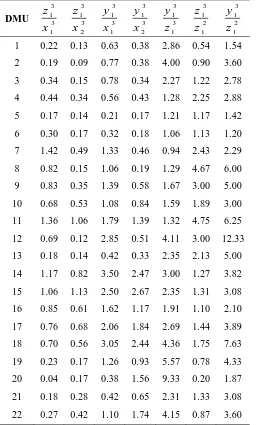
Table 6. Data related to the 22 Iranian medical centers in summer 2016 (stage 3)
Therefore, we can easily evaluate the units using the suggested network DEA-R model. Using the structure of MOLP in three-stage network DEA-R has the following outcomes:
a) By considering P1M1, P2M2 and
3
3 M
P in model (17) where
1 3 2 1M M
M and M1,M2,M3
0,1efficiency value of each process would be calculated separately.
b) If M1,M2,M3
0,1 in model (17), we would arrive at the overall efficiency and the evaluation criterion would depend on the values of M1, M2 and M3.DMU
3 1 3 1
z
x
3 1 3 2
z
x
3 1 3 1
y
x
3 1
3 2
y
x
3 1
3 1
y
z
3 1 2 1
z
z
3 1 2 1
y
z
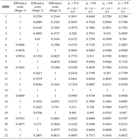
Table 7. Comparison of efficiency values obtained from model (17) using different parameters
DMU
Efficiency score (Stage 1)
Efficiency score (Stage 2)
Efficiency score (Stage 3)
4 . 0
3
p p10.8 p20.8 p3 0.8
p1 = p2 =
0.3
p2 = p3 =
0.1
p1 = p3 =
0.1
p1 = p2 =
0.1 1 1 0.2556 0.2164 0.3011 0.6049 0.2709 0.2388 2 1 0.6089 0.3365 0.5047 0.7928 0.5844 0.3786 3 1 0.6105 0.3283 0.4975 0.7884 0.5831 0.3702 4 1 0.4003 0.4737 0.528 0.7931 0.433 0.4905 5 1 0.61 0.2456 0.4132 0.7294 0.5499 0.284 6 0.9086 1 0.2386 0.4335 0.7145 0.7523 0.2807 7 0.9878 1 1 0.9963 0.9903 0.9988 0.9988 8 0.9974 0.5158 0.9825 0.7755 0.911 0.5705 0.9022 9 1 1 0.6876 0.8462 0.9566 0.9566 0.7335 10 0.3662 1 0.5206 0.5298 0.4038 0.7904 0.5236 11 1 0.2617 1 0.5416 0.7799 0.307 0.7799 12 1 0.3519 1 0.6441 0.8444 0.4043 0.8444 13 1 0.8564 0.5442 0.7218 0.9087 0.8211 0.5928
14 1 1 1 1 1 1 1
15 0.9689 1 1 0.9905 0.9749 0.9968 0.9968 16 1 0.3034 0.6591 0.5275 0.7805 0.3462 0.6085 17 1 0.2642 0.767 0.511 0.764 0.3069 0.6572
18 1 0.9706 1 0.991 0.997 0.9763 0.997
19 0.9343 1 0.4861 0.6925 0.8606 0.8987 0.5397 20 0.4877 0.272 0.5846 0.4162 0.4589 0.3014 0.5151 21 1 1 0.3975 0.6226 0.8684 0.8684 0.452 22 1 0.2607 0.6813 0.4907 0.7517 0.3016 0.6032
Model (17) is a linear programming problem;
p
1,p
2 andp
3 are determining parameters for overall efficiency of the three-stage network process.Firstly, due to the priority of stage 1 compared to other stages, p11 and
0
3 2p
p , meaning that
n
j
j p
1
1 1
1
.
Therefore, based on the categorization of
I
,F
&R
for the first stage, we canpatients receive quality services in the surgery stage, but chemotherapy and radiotherapy stages lack proper service provision.
After a detailed study of stages 2 & 3, we arrived at the following issues:
a) Due to drug shortages and inability of patients to receive drugs (in terms of weak immune systems and allergic reactions to drugs), the chemotherapy stage requires special attention.
b) The services provided in the radiotherapy stage lack quality due to the high number of patients, their desire for liberation from the treatment process (pain & suffering during treatment & disease) and problems with radiotherapy devices.
Therefore, it is of great importance in this stage to fix the issues with radiotherapy machines, train the personnel to provide better services, convince the patients to stick to timetables in between radiotherapy sessions and make them aware of the dangers of radiotherapy. Columns 5 to 8 from Table 7 present the overall efficiency obtained from model (17).
Four groups of weights were selected for the vector
p1,p2,p3
:Group 1: Equal priority for all three network stages with parameters
p1,p2,p3
0.3,0.3,0.4
. Unit 14 is the only efficient one, however, units 7, 15 & 18 are closer to being efficient.Group 2: Priority of the first stage in all three stages and finding the Pareto efficient solution using parameters
p1,p2,p3
0.8,0.1,0.1
. Unit 14 is theonly one efficient, however, units 7, 8, 9, 13 & 15 are closer to efficiency.
Group 3: Priority of the second stage in all three stages and finding the Pareto efficient solution using parameters
p1,p2,p3
0.1,0.8,0.1
. But units 7, 9, 15 & 18 are closer to efficiency.Group 4: Priority of the third stage in all three stages and finding the Pareto
efficient solution using parameters
p1,p2,p3
0.1,0.1,0.8
. But units 7, 15 & 18 are closer to efficiency.As can be witnessed in figures 5, 6 & 7, the first stage has similar behavior to the overall efficiency of the network, but stages 2 & 3 aren’t similar, therefore the medical centers don’t have an overall high efficiency. Since only unit 14 is efficient, the first stage has good efficiency but the second and third stages showed weak performances. Therefore, it’s essential to revise the process of treatment in stages 2 & 3.
6. Conclusions
DEA-R models (a combination of DEA and ratio data) are used in data envelopment analysis for evaluation of decision-making units, when inputs and outputs are not available and we only have access to a defined ratio of data. In many DMUs, intermediate links play an important role in the network structure of DEA. Therefore, we evaluated 22 medical centers in this paper using network DEA-R models based on the structure of MOLP. Therefore, the reasons for using a three-stage network DEA-R model are as follows:
I) When
x
j,y
j andz
j are not available for DMUj in all three-stages and we only have access to a ratio ofj j
x z
and
j j
z y
, network DEA-R models can be a suitable alternative for network DEA.
were efficient in stage 2 and 27% became efficient in stage 3. However, based on overall efficiency, unit 14 was the only one deemed efficient. With an optimistic view of model (17)’s optimal solutions (columns 5 to 8 of Table 7), we can say that units 6, 15 & 18 had proper performances in all three stages; on this basis, 18% of the units were approved in all stages based on overall efficiency value. Finally, our overall suggestions for the studied medical centers are as follows: a) The first stage of treatment requires the most attentive service provision; most of the centers, except units 10 & 20, had an acceptable performance in the first stage (Surgery).
b) The second stage (Chemotherapy) requires even more attention in service provision. In this regard, units 6, 7, 9, 10, 14, 15 & 19 were efficient and units 1, 11, 12, 16, 17, 20 & 22 had weak performances. Those centers need to receive necessary training on service provision, patient guidance and drug prescription.
References
Banker, R.D., Charnes, A. and Cooper, W.W. (1984). Some models for estimating technical and scale inefficiencies in data envelopment analysis. Management Science, 30 (9), 1078-1092.
Charnes, A., Cooper, W.W. and Rhodes, E. (1978). Measuring the efficiency of decision making units. European Journal of Operational Research, 2 (6), 429-444. Chen, C. and Yan, H. (2011). Network DEA model for supply chain performance evaluation. European Journal of Operational Research, 213 (1), 147–155. Chen, C., Zhu, J., Yu, J.Y. and Noori, H. (2012). A new methodology for evaluating sustainable product design performance with two-stage network data envelopment analysis. European Journal of Operational Research, 221 (2), 348– 359.
Chen, Y., Cook, W.D., Li, N. and Zhu, J. (2009). Additive efficiency decomposition in two-stage DEA. European Journal of Operational Research, 196 (3), 1170–1176.
Chen, Y., Liang, L. and Yang, F. (2006). A DEA game model approach to supply chain efficiency. Annals of Operations Research, 145 (1), 5-13.
Cook, W.D. and Zhu, J. (2014). Data envelopment analysis - a handbook of modeling internal structure and network. New York: Springer.
Cook, W.D., Zhu, J., Bi, G. and Yang, F. (2010). Network DEA: Additive efficiency decomposition. European Journal of Operational Research, 207 (2), 1122-1129.
Despic, O., Despic, M. and Paradi, J.C. (2007). DEA-R: Ratio-based comparative efficiency model, its mathematical relation to DEA and its use in applications. Journal of Production Analysis, 28 (1-2), 33-44.
Despotis, D. K., Koronakos, G. and Sotiros, S. (2015). A multi-objective programming approach to network DEA with an application to the assessment of the academic research activity. Procedia Computer Science, 55, 370–379.
Despotis, D. K., Koronakos, G. and Sotiros, D. (2016a). The “weak-link” approach to network DEA for two-stage processes. European Journal of Operational Research, 254 (2), 481-492. Despotis, D. K., Koronakos, G. and Sotiros, D. (2016b). Composition versus decomposition in two-stage network DEA: A reverse approach. Journal of Production Analysis, 45 (1), 71–87. Despotis, D.K., Sotiros, D. and Koronakos, G. (2016c). A network DEA approach for series multi-stage processes. Omega, 61 (1), 35-48.
Färe, R. and Grosskopf, S. (1996). Productivity and intermediate products: A frontier approach. Economics Letters, 50 (1), 65-70.
Färe, R. and Grosskopf, S. (2000). Network DEA. Socio-Economic Planning Sciences, 34 (1), 35–49.
Farrell, M.J. (1957). The measurement of productive efficiency. Journal of the Royal Statistical Society. Series A (General), 120 (3), 253-290.
efficiency in two-stage additive network DEA. European Journal of Operational Research, 257 (3), 896–906.
Kao, C. and Hwang, S.N. (2008). Efficiency decomposition in two-stage data envelopment analysis: An application to non-life insurance companies in Taiwan. European Journal of Operational Research, 185 (1), 418– 429.
Kao, C. (2009). Efficiency decomposition in network data envelopment analysis: A relational model. European Journal of Operational Research, 192 (3), 949–962. Kao, C. (2014a). Efficiency decomposition for general multi-stage systems in data envelopment analysis. European Journal of Operational Research, 232 (1), 117–124.
Kao, C. (2014b). Network data envelopment analysis: A review. European Journal of Operational Research, 239 (1), 1–16.
Li, Y., Chen, Y., Liang, L. and Xie, J. (2012). DEA models for extended two-stage network structures. Omega, 40 (5), 611–618.
Liang, L., Cook, W.D. and Zhu, J. (2008). DEA models for two-stage processes: Game approach and efficiency decomposition. Naval Research Logistics, 55 (7), 643–653.
Liu, W.B., Zhang, D.Q., Meng, W., Li, X.X. and Xu, F. (2011). A study of DEA models without explicit inputs. Omega, 39 (5), 472–480.
Mozaffari, M.R., Gerami, J. and Jablonsky, J. (2014a). Relationship between DEA models without explicit inputs and DEA-R models. Central
European Journal of Operations Research, 22 (1), 1-12.
Mozaffari, M.R., Kamyab, P., Jablonsky, J. and Gerami, J. (2014b). Cost and revenue efficiency in DEA-R models. Computers & Industrial Engineering, 78, 188-194.
Olesen, O.B., Petersen, N.C. and Podinovski, V.V. (2015). Efficiency analysis with ratio measures. European Journal of Operational Research, 245, 446-462.
Wei, C.K., Chen, L.C., Li, R.K. & Tsai, C.H. (2011a). A study of developing an input-oriented ratio-based comparative efficiency model. Expert Systems with Applications, 38 (3), 2473-2477.
Wei, C.K., Chen, L.C., Li, R.K. & Tsai, C.H. (2011b). Exploration of efficiency underestimation of CCR model: Based on medical sectors with DEA-R model. Expert Systems with Applications, 38 (4), 3155-3160.