Quality Improvement Through Multiple Response Optimization (TECHNICAL NOTE)

TECHNECAL NOTE

QUALITY IMPROVEMENT THROUGH

MULTIPLE RESPONSE OPTIMIZATION

R. Noorossana

Department of Industrial Engineering, Iran University of Science and Technology Tehran 16844 Iran, [email protected]

H. Alemzad

Alka Ravesh Company

Tehran 19697 Iran, [email protected]

(Received: August 8, 2001 - Accepted in Revised Form: December 12, 2002)

Abstract The performance of a product is often evaluated by several quality characteristics. Optimizing the manufacturing process with respect to only one quality characteristic will not always lead to the optimum values for other characteristics. Hence, it would be desirable to improve the overall quality of a product by improving quality characteristics, which are considered to be important. The problem consists of optimizing several responses using multiple objective decision making (MODM) approach and design of experiments (DOE). A case study will be discussed to show the application of the proposed method.

Key Words Multi-response Optimization, Multi Objective Decision Making, Goal Programming, Capability Index, Statistical Process Control, Design of Experiments

ﻩﺪﻴﻜﭼ

ﻩﺪﻴﻜﭼ

ﻩﺪﻴﻜﭼ

ﻩﺪﻴﻜﭼ

ﺩﻮﺷ ﻲﻣ ﻲﺑﺎﻳﺯﺭﺍ ﻲﻔﻴﻛ ﻪﺼﺨﺸﻣ ﻦﻳﺪﻨﭼ ﺱﺎﺳﺍ ﺮﺑ ﹰﺎﺒﻟﺎﻏ ﻝﻮﺼﺤﻣ ﻚﻳ ﺩﺮﻜﻠﻤﻋ .

ﺪﻨﻳﺁﺮﻓ ﻚﻳ ﻱﺯﺎﺳ ﻪﻨﻴﻬﺑ

ﺎﺑ ﺪﻴﻟﻮﺗ ﺪﺷ ﺪﻫﺍﻮﺨﻧ ﻲﻔﻴﻛ ﻱﺎﻫ ﻪﺼﺨﺸﻣ ﺮﻳﺎﺳ ﻥﺪﺷ ﻪﻨﻴﻬﺑ ﻪﺑ ﺮﺠﻨﻣ ﻪﺸﻴﻤﻫ ﻲﻔﻴﻛ ﻪﺼﺨﺸﻣ ﻚﻳ ﻂﻘﻓ ﻦﺘﻓﺮﮔ ﺮﻈﻧ ﺭﺩ .

ﺩﻮﺷ ﻱﺯﺎﺳ ﻪﻨﻴﻬﺑ ﻥﺁ ﻢﻬﻣ ﻲﻔﻴﻛ ﻱﺎﻫ ﻪﺼﺨﺸﻣ ﻪﻴﻠﻛ ﻪﺑ ﻪﺟﻮﺗ ﺎﺑ ﻝﻮﺼﺤﻣ ﻚﻳ ﺖﻴﻔﻴﻛ ﺎﺗ ﺩﺩﺮﮔ ﻲﻌﺳ ﺪﻳﺎﺑ ﻦﻳﺍ ﺮﺑﺎﻨﺑ .

ﻱﺮﻴﮔ ﻢﻴﻤﺼﺗ ﺩﺮﻜﻳﻭﺭ ﻪﻠﻴﺳﻭ ﻪﺑ ﺦﺳﺎﭘ ﺮﻴﻐﺘﻣ ﻦﻳﺪﻨﭼ ﻱﺯﺎﺳ ﻪﻨﻴﻬﺑ ﻞﻣﺎﺷ ﺮﻈﻧ ﺩﺭﻮﻣ ﻪﻟﺎﺴﻣ ﻪﻓﺪﻫ ﺪﻨﭼ

) MODM ( ﻭ

ﺎﻬﺸﻳﺎﻣﺯﺁ ﻲﺣﺍﺮﻃ )

DOE ( ﺪﺷﺎﺑ ﻲﻣ . ﻪﻳﺰﺠﺗ ﺩﺭﻮﻣ ﻱﺩﺭﻮﻣ ﻪﻌﻟﺎﻄﻣ ﻚﻳ ﻱﺩﺎﻬﻨﺸﻴﭘ ﺵﻭﺭ ﺩﺮﺑﺭﺎﻛ ﻥﺩﺍﺩ ﻥﺎﺸﻧ ﺭﻮﻈﻨﻣ ﻪﺑ

ﺖﻓﺮﮔ ﺪﻫﺍﻮﺧ ﺭﺍﺮﻗ ﻞﻴﻠﺤﺗ ﻭ .

1. INTRODUCTION

The overall value of a manufactured product is usually determined with respect to several quality characteristics or responses of interest. These responses are often interrelated and need to be considered simultaneously. For the case of a single response, design of experiments methods can be employed to analyze data and determine the optimum operating levels for process parameters, which influence the response. However, for the case of two or more responses, process optimization

by means of optimizing only one characteristic at a time often results in non-optimal or even unacceptable values for other quality characteristics.

In multi-response experiments usually a combination of the following three types of responses are considered:

1. Responses that we like them to be minimized (Lower The Better - LTB)

2. Responses that are required to be maximized (Higher The Better - HTB)

Hence, we can easily encounter an experiment in which the responses of interest are in contrast with each other and reaching a solution that optimizes all of these characteristics is usually impossible. Therefore, a compromise solution that improves these responses is desired. Simultaneous optimization techniques are mathematical procedures that can be helpful for the analysis of multi-response experiments in order to determine the optimum operating condition. This is the operating condition at which all quality characteristics are as close to their nominal values as possible.

Simultaneous consideration of multiple responses involves first building an appropriate response surface model for each response and then trying to find a set of operating conditions which in some sense optimizes all responses or at least keeps them in desired ranges (Montgomery [1]). Figure 1 summarizes the main steps in multiple response experiments.

The desirability function approach to multi-response optimization is one of the most commonly used techniques for the analysis of experiments in which several quality characteristics must be optimized simultaneously. This method was first developed by Harrington [2] and later was modified by Derringer and Suich to improve its

performance [3]. The latter method ignores the variability of the response variables and this can be considered as its major drawback. Goik et al. [4] compensates for this problem by incorporating variation in the desirability function.

The basic idea of the desirability function approach is to transform a multi-response problem into a single response problem by means of mathematical transformations. In this approach, for each response Yi (x), i = 1, 2, …, p, a function

di(Yi(x)) with range of values between 0 and 1 is

defined that measures how desirable it is that Yi(x)

takes on a particular value. Here x = (x1, x2, x3, …,

xk) denotes the vector of controllable or independent

factors. Once the desirability function for each response variable is defined, an overall objective function D(x) is defined as the geometric mean of

the individual desirability.

( )

[

( )

( )

( )

]

1 p p p 2

2 1

1Y d Y d Y

d

D x = x x _L x (1)

The reason for considering the geometric mean is that if any quality characteristic has an undesirable value (i.e., d_i

(

Y_i

( )

x

)

= 0) at some

treatment combination or operating condition x = x0

then the overall performance of the manufactured

Step 1- Performing experiment using suitable designs such as factorial, fractional factorial or

central composite designs

Step 2- Obtaining significant regression models for predicting response values according to

control variable settings.

Step 3- Choosing the utility or value criterion for transforming response values to these

criterions which enables one to effectively and correctly compare different control variable

settings.

Step 4- Determining bounds, targets, weights, priorities, etc. for each response.

Step 5- Modeling the problem and using the resulting model to optimize responses through

specified criterions by changing control variable levels.

Step 6- Optimizing the model by using an appropriate optimization technique.

product is unacceptable, regardless of the values taken by the remaining response variables.

Box, Hunter and Hunter [5] considered using overlaying contour plots. This graphical method is also widely used since it can be easily performed and results are also easy to interpret but it has two major disadvantages. First, it is not applicable when we have more than two process variables and its’ interpretation becomes difficult when the number of response variables increases to more than three. Second, contour plots are incapable of showing inherent errors. In this method, decisions are mostly made subjectively.

Many researchers have used Taguchi’s loss function as a value criterion in optimization of several responses. For example, Artiles-Leon [6] uses a dimensionless loss function for combining several loss functions associated with different response variables and uses this method to optimize a plastic molding process. Pignatiello [7] expanded Taguchi’s loss function to a multivariate loss function and presented a method based on minimization of deviation from target and maximization of robustness to noise. Elsayed and Chen [8] proposed a two-step method using Taguchi’s loss function. Many authors including Jayaram and Ibrahim [9], Kunjur and Krishnamurti [10] have also considered Taguchi’s loss function in their studies.

Jayaram and Ibrahim [11] introduced a method by using Cp and Cpk capability indices as desirability

criteria. Khuri [12] introduced a new multi-response optimization approach based on a multivariate metric called Mahalanobis distance. His proposed distance metric is nearly the squared deviation of responses from their desired targets, normalized by the variance of the predicted responses. He is among the researchers who have published many articles in the area of multi-response optimization. Interested readers are referred to Khuri and Conlon [12], Khuri and Cornell [13], and Khuri [14]. In the area of problem formulation and modeling, some researchers have applied multi-criteria decision making (MCDM) techniques for obtaining a compromise solution in multi-response optimization. Chang and Shivpuri [15] used an MODM technique for optimizing both casting quality and die life in a die casting process. In their work, they used desirability function proposed by Derringer and Suich [3] as the desirability criterion. Tang and Su

[16] considered Technique for Order Preference by Similarity to Ideal Solution (TOPSIS) method to optimize a multi-response problem. Fogliatto [17] and Reddy [18] used Saati’s Analytical Hierarchy Process (AHP) and goal programming in multi-response optimization, respectively. Multi Attribute Decision Making (MADM) techniques are used for selecting between several existing alternatives and therefore their application for optimizing multi-response experiments is only suggested when a significant regression model is not available.

Another MCDM technique that has been considered in optimization problems is the multi-criteria steepest ascent method based on MCDM/PO (Duineveld and Coenegracht [19]). Briefly, in this method the steepest ascent direction that simultaneously optimizes the response variables is determined by identifying Pareto Optimal (PO) points on the common PO plot. Experimentation will be continued on this direction until no further improvement is perceived.

Some other techniques and procedures are also available in the literature, each having its own strengths and weaknesses. Some important issues that should be considered in multi-response techniques are:

1. Simplicity and ease of application.

2. Consideration of variability and correlation of responses.

3. Interactivity.

4. Flexibility of solutions.

The method proposed in this paper tries to incorporate these issues in the optimization problem.

In this paper, we propose a new approach for optimization and analysis of experiments with multiple responses based on the capability index Cpm, which is often considered in process

capability analyses. This index is used as a utility criterion for assessing each response and then with the aid of MODM goal programming technique we try to determine an optimum solution for the process variables.

General formulation of multi-response models is reviewed in the next section. In the third section, the Cpm index is discussed. The fourth section

2. GENERAL FORMULATION OF MULTI-RESPONSE MODELS

In general, formulation of the multi-response models starts with designing experiments and collecting information on each of the response variables Y_i, i = 1, 2, …, p for each treatment combination of design variables (Xj’s, j = 1, 2, …,

k). Total number of treatments is denoted by t. Each response is related to a set of design variables by the following functional relationship:

(

1 2 k

)

ij

i

ij

f

X

,

X

,

,

X

Y

=

K

+

ε

i = 1, 2, …, p

j = 1, 2, …, k (2) In the above equation, the error term, ε_ij, is normally and independently distributed with mean zero and variance σ_ij2.

Let Y(x) denote the 1p× vector of the

responses at a particular setting of the X’s in the experimental region denoted by x. Expected value

of the response vector Y(x) is a p×1 vector

shown by η(x). Mean of the ith response at a

particular setting x, ηi(x) is estimated by a

regression model. Let r denote the number of regression coefficients. The regression model for the response variable i at x is defined by:

i i( ) z( )βˆ

Yˆ x = ′ x (3)

where βˆ_i is a r×1 vector of regression coefficient estimates and z′(x) is an r×1 vector of regression variables. These regression variables may be main effect terms, cross-product terms, and squared terms as needed by the selected model. For example, z′(x) can be equal to

(

1,x1,x2,x1x2,x12

)

.

The variance-covariance of Y_i(x) is shown by the p×p matrix

∑

( )

x . If variance of response

variables are equal for all treatments, then

( )

∑

∑

x = . Let S_y(x) denote the estimate of

( )

∑

x and let

∑

ˆ

be the estimator for

∑

.

The p×1 vector of target values for the

response is defined by ττττ . Let ub and lb be p×1 vectors of the upper and lower bounds, respectively, for the acceptability region of the response variables. Any response value outside this region is considered unacceptable.

Our proposed approach uses a process capability index denoted by Cpm for assessing each setting of

process variables considering both optimality of the response value and variability of the responses in that particular setting (Robustness). Before proceeding to model formulation using the Cpm

capability index as an optimization criterion, we need to discuss few issues related to this index.

3. THE CPM INDEX

Chan et al. [20] suggested first the capability index, Cpm, sometimes referred to as the Taguchi

index. This index gives a single numerical value, which pictures the total performance of a process and depends on both variability and deviation from target (centering). It ensures that conditions of centering and variability are satisfied. The Cpm

index is defined by

(

)

[

2 2

]

1 2

6 σσσσ µµµµ Target LSL USL C_pm

− +

−

= (4)

The loss function appears in the denominator. The term ₆

[

2

(

)

2

]

12

Target

µ µµ µ σ σσ

σ + − gives average loss per piece for a sample.

The Cpm index is equal to the traditional

capability index Cp when the process is perfectly

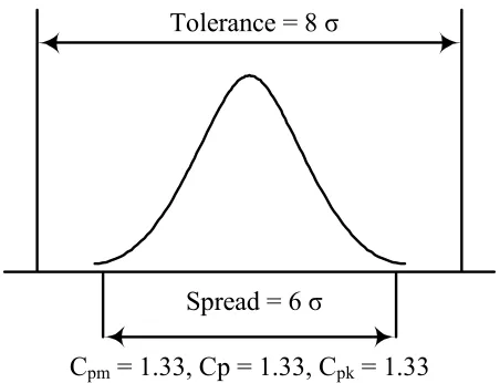
centered between the upper and lower specification limits. The Cpm index begins to decrease as the

process mean shifts away from the pre-specified target value or the process variability increases. Figure 2 presents a reference situation corresponding to the maximum acceptable loss in the case of a normal distribution. This situation refers to a centered production when Cpm = Cp = Cpk = 1.33.

To avoid generating a loss (according to Taguchi) superior to the reference situation, the Cpm must

remain superior to 1.33.

The Cpm index proposed by Chan et al. [20] is

specification limits for the process and a target which is usually at the center of the upper and lower tolerance interval. In many cases we are faced with process characteristics, which have unilateral tolerance limits (LTB and HTB). Pillet et al. [21] proposed a Cpm index for the case of

unilateral tolerances bounded by zero. Their proposed Cpm index is defined as:

[

_{2 2}

]

1 2

A Tolerance X σ σσ σ Cpm +

= (5)

where σ is the standard deviation of the population X is the mean of the population, A is a constant

that depends on the desired quality. Pillet et al. [21] recommended using A = 1.46 and they justify that this value ensures a good quality level.

In our proposed approach, we use Cpm as an

index for assessing desirability of responses at each setting of control variables (factors). For the bilateral case, we use

( )

( )

(

( )

)

[

₂

]

12

i i 2 i i i i, pm ˆ ˆ 6 lb ub C ττττ x x x − η + σ −

= (6)

For the unilateral case when higher-the-better type

response is considered Cpm is defined as

( )

( )

(

( )

)

[

]

12

i max 2 i i max i , pm ˆ y ˆ 46 . 1 lb y C x x x η − + σ −

= (7)

and for lower-the-better type response Cpm can be

defined as

( )

( )

(

( )

)

[

_min

]

12

i 2 i min i i , pm y ˆ ˆ 46 . 1 y ub C − η + σ − = x x

x (8)

In the above equations, C_pm,i(x) denotes the Cpm

index value for ith response at control variables setting x. The quantities ubi and lbi are the upper

and lower limits for ith response, respectively.

( )

x

2 i

ˆ

σ and ηˆ_i

( )

x are the variance and mean of the

ith predicted response at setting x, and

τ

_i denotes

the desired target for the ith _response.

The variance of the predicted response (σˆ_i2

( )

x )

is derived from the following equation:

( )

(

)

[

( )

]

( )

[

0 0

]

2 0 0 2

x

X

X'

x

x

X

X'

x

x

'

'

1

ˆ

'

'

1

p

t

yˆ

y

ˆ

1 1 i n 1 i 2 i i i − − =

+

σ

=

+

























−

−

=

σ

∑

(9)

where

t

is number of treatments and

p_i

is the

number of regression coefficients for response i.

When C

pm

is utilized as a value function for

assessing the response variables the following

advantages can be expected:

1. Since the variability of the response is considered the performance of the index will be superior to Derringer and Suich's desirability function and also other methods that only focus on the centering of the responses.

2. It is relatively easier to understand and it can be compared to many other methods such as Khuri and Cornell [12], Pignatiello [7] and Oh [22]. This index is also applied in process capability studies in statistical process control (SPC) programs and it can be easily computed

Tolerance = 8

σ

Spread = 6

σ

C

pm

= 1.33, Cp = 1.33, C

pk

= 1.33

by most statistical packages.

3. This index considers both deviation from target and variability in one single value and therefore it is superior to the method suggested by Jayaram and Ibrahim [11].

4. THE PROPOSED OPTIMIZATION APPROACH

In this section, the problem will be formulated and solved as a non-linear goal-programming (NLGP) model. NLGP is a multiple objective decision making technique in which all objectives are considered as constraints in the model and a numerical goal level (ideal) is specified for each constraint. Goal constraints are conditions that are desired, but not required. For each objective (goal constraint) a positive and a negative deviation variable will be specified. The model will be optimized for minimizing the summation of these deviation variables. Weights can also be used in this procedure to indicate the proportional importance of each objective. The aim of goal programming is to minimize

(

)

∑

=

− − +

+

+

=

m 1 i

i i i

i

d

w

d

w

z

₍₁₀₎

Subject to:

( )

d d g i

fi x + i−− i+= i ∀ (11)

i 0

d ,

d_i+ _i− ≥ ∀

The proposed approach in optimization of multi-response experiments is summarized as follows. 1. Specifying the process parameters to study

and determine their ranges and levels. 2. Specifying the response variables.

3. Using DOE techniques and response surface methodology to obtain empirical models for

i

Y where i=1,2,…,p for predicting the response values as a function of control variables x.

4. Specifying the upper and lower bounds and target for the responses (ubi, lbi, and τi).

a. In case of NIB responses, the target is usually

in the middle of the specification limits. b. In case of HTB (LTB) responses, the target is defined as _ymax

( )

_ymin _{and is determined}

through solving the following model for the response:

(

Minimize

)

z ηˆ

( )

x

Maximze = _i (12)

Subject to:

( )

j

{

(

1,...,p

)

j i

}

ˆ

j

j x ≤ub ∈ ≠

ηηηη (13)

( )

j

{

(

1,...,p

)

j i

}

ˆ

j

j x ≥lb ∈ ≠

ηηηη (14)

X

x

∈

5. Specifying the desired goals for Cpm,i(x)

indices (Cpm,i*(x)).

6. Applying NLGP methodology to formulate a problem for minimizing deviation of each of the Cpm,i(x) indices from its specified goal

(Cpm,i*(x)).

Minimize:

∑

=

− − = m

1 i

i id

w

z (15)

Subject to:

( )

d C i

C_{pm,i x} + _i− = _pm,i∗ ∀ ₍₁₆₎

i 0

d_i ≥ ∀

∈ −

X, x

7. Solving the NLGP model with an appropriate optimization method to obtain a compromise solution (x∗).

8. Performing verification experiments in the optimum setting acquired in the previous step to confirm the achieved results.

9. Applying the new setting to the process and start a statistical process control program to maintain the results.

5. A CASE STUDY

and results will be compared to two other methods from the literature. We use the problem presented by Montgomery [1] for simultaneous optimization of a chemical process.

In this problem the aim is to identify process settings in order to simultaneously optimize three quality characteristics, process yield (Y1), viscosity

(Y2), and molecular weight (Y3) such that yield is

maximized, viscosity is set on a specified target, and molecular weight is minimized (see Table 1 for details).

Two process parameters, reaction time (x1) and

reaction temperature (x2), were considered to have

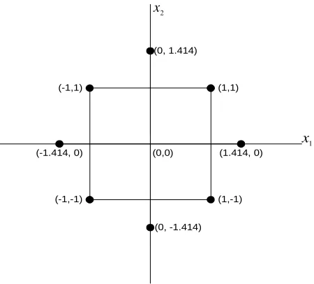
the maximum effect on these three responses. The central composite design (CCD) shown in Figure 3

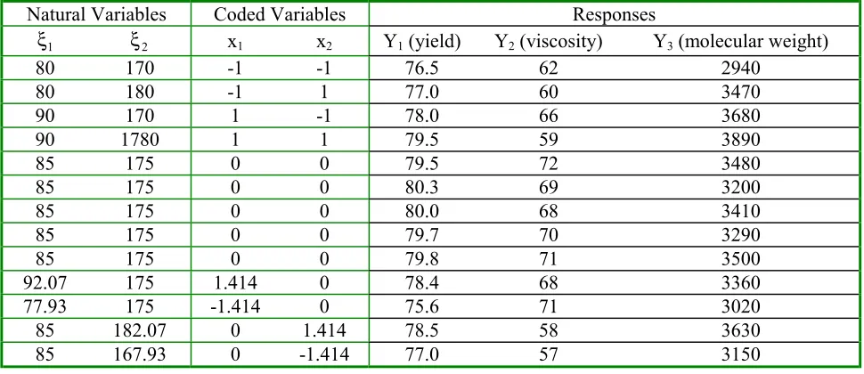
was used to assess the relationship between these process parameters (Factors) and the selected responses. The experimental settings along with the data are shown in Table 2.

Using multiple regression technique, the

following models will be achieved for yield,

viscosity and molecular weight responses,

respectively:

2 1 2

2 2

1

2 1

1

x x 25 . 0 x 00 . 1 x 38 . 1

x 52 . 0 x 99 . 0 94 . 79 Yˆ

+ −

−

+ +

=

(17)

2 1 2

2 2

1

2 1

2

x x 25 . 1 x 69 . 6 x 69 . 0

x 95 . 0 x 16 . 0 00 . 70 Yˆ

− −

−

− −

=

(18)

2 1

3 3386.2 205.1x 17.4x

Yˆ = + + (19)

Now, we solve the problem and compare the results to the results obtained from following two alternatives:

1. Derringer and Suich's desirability function approach (DS)

2. Chang and Shivpuri's MODM Approach (CS) We used MS-Excel 97 software for solving the problem using each of the three approaches. The NLGP model we used for this problem is:

Minimize: z=

(

w1−d1− +w2−d2− +w3−d3−

)

(20)

TABLE 1. Response Variables.

Dependent Variables Description Unit Type Lower Bound Target Upper Bound

1

Y Process Yield % HTB 70 79.33* --

2

Y Viscosity (cc) NIB 62 65 68

3

Y Temperature Difference (°F) LTB -- 2927.21* ₃₄₀₀

* The Target values for Y₁ andY₃ were determined as suggested in step 4 of the proposed approach.

(-1,1) (1,1)

(1,-1) (-1,-1)

(0,0) (1.414, 0) (0, 1.414)

(-1.414, 0)

(0, -1.414)

1

x

2

x

Subject to:

( )

i 0

d ,

i C

d x C

i

* i , pm i i , pm

∀ ≥

∀ =

+ −

−

x

(21)

According to this table, the model outperforms the other two models with respect to the standard deviation uniformly, which is an important issue in robust design problems. However, the model does not perform equally well in terms of the means. In general, these results indicate that the proposed approach is capable of providing a relatively better solution than the other two approaches in terms of the rate of non-conformity (%N/C). Table 4

compares the rate of non-conformity in responses resulted from the proposed approach to those obtained from the Derringer and Suich's and Chang and Shivpuri's approaches. The algebraic sum for the differences of each response is shown in the last column denoted by Σ.

6. CONCLUSIONS

This paper is concerned with enhancement of quality through multi-response optimization. The vehicles used to accomplish this goal are a common process capability index known as Cpm

TABLE 2. Experimental Runs.

Natural Variables Coded Variables Responses

1

ξ ξ₂ x1 x2 Y1 (yield) Y2 (viscosity) Y3 (molecular weight)

80 170 -1 -1 76.5 62 2940

80 180 -1 1 77.0 60 3470

90 170 1 -1 78.0 66 3680

90 1780 1 1 79.5 59 3890

85 175 0 0 79.5 72 3480

85 175 0 0 80.3 69 3200

85 175 0 0 80.0 68 3410

85 175 0 0 79.7 70 3290

85 175 0 0 79.8 71 3500

92.07 175 1.414 0 78.4 68 3360

77.93 175 -1.414 0 75.6 71 3020

85 182.07 0 1.414 78.5 58 3630

85 167.93 0 -1.414 77.0 57 3150

TABLE 5. Optimal Solutions Resulting from the Proposed Approach, the Derringer Method, and the MODM Technique.

%N/C Method x1 x2 Yˆ₁ Yˆ₂ Yˆ₃ σˆ1 σˆ2 σˆ3

1

Yˆ Yˆ₂ Yˆ₃

Proposed

and goal programming as an optimization technique. Although, many optimization techniques have been used or developed by researchers (see for example, Wurl and Albin [23], Del Castillo, Montgomery, and McCrville [24], Del Castillo [25], Das [26], Fogliatto and Albin [27], and Carlyle, Montgomery, and Runger [28]) for optimization purposes but we used goal programming because of its flexibility and its’ applicability to real world engineering problems.

Using a set of data from Montgomery [1], the performance of the proposed model was evaluated against two other methods suggested by Derringer and Suich [3] and Chang and Shivpuri [15]. The results indicated a better performance for the proposed model. Future work is necessary not only to determine the weights and goals analytically but also to provide a methodology that utilizes the possible correlation that might be present between responses.

7. ACKNOWLEDGMENT

The authors would like to thank the two anonymous referees for their helpful comments and suggestions, which led to improvements in our original manuscript.

8. REFERENCES

1. Montgomery, D. C., “Design and Analysis of Experiments”, 4th _{Edition, John Wiley and Sons, New}

York, (2001).

2. Harrington, E. C. Jr., “The Desirability Function”,

Industrial Quality Control, Vol. 21, (1965), 494-498.

3. Derringer, G. and Suich, R., “Simultaneous Optimization

of Several Response Variables”, Journal of Quality Technology, Vol. 12, (1980), 214-219.

4. Goik, P., Liddy, J. W. and Taam, W., “Use of Desirability Functions to Determine Operating Windows for New Product Designs”,Quality Engineering, Vol. 7,

No. 2, (1995), 267-276.

5. Box, G. E. P., Hunter, W. G. and Hunter, J. S., “Statistics for Experimenters: an Introduction to Design, Data Analysis and Model Building”, John Wiley and Sons, New York, (1978).

6. Artiles-Leon, N., “A Pragmatic Approach to Multiple-Response Problems Using Loss Functions”, Quality Engineering, Vol. 9, No. 2, (1995), 213-220.

7. Pignatiello, J. J. Jr., “Strategies for Robust Multi-Response Quality Engineering” IIE Trans., Vol. 25,

(1993), 5-15.

8. Elsayed, E. A. and Chen, A., “Optimal Levels of Process Parameters for Products with Multiple Characteristics”,

International Journal of Production Research, Vol. 31,

No. 5, (1993), 17-32.

9. Jayaram, J. S. R. and Ibrahim, Y., “Robustness for Multiple Response Problems Using a Loss Model”,The International Journal of Quality Science, Vol. 2, No. 3,

(1997), 199-205.

10. Kunjur, A. and Krishnamurthy, S., “A Multi-Criteria Based Robust Design Approach”, Technical Report,

Department of Mechanical Eng., University of Massachusetts, (1997).

11. Jayaram, J. S. R. and Ibrahim, Y., “Multiple Response Robust Design and Yield Maximization”, International Journal of Quality and Reliability Management, Vol. 16, No. 9, (1999), 826-837.

12. Khuri, A. I. and Conlon, M., “Simultaneous Optimization of Multiple Responses Presented by Polynomial Regression Functions”, Technometrics, Vol. 23, (1981), 363-375.

13. Khuri, A. I. and Cornell, M., “Response Surfaces”, Marcel Dekker, Inc., New York, (1987).

14. Khuri, A. I., “Recent Advances in Multi-response Design and Analysis”, Technical Report #599, Department of

Statistics, University of Florida, Gainesville, Florida, (1999).

15. Chang, S. I. and Shivpuri, R., “A Multiple-Objective Decision Making Approach for Assessing Simultaneous Improvements in Die Life and Casting Quality in a Die Casting Process”,Quality Engineering, Vol. 7, No. 2,

(1995), 371-383.

TABLE 4. Comparison of the Proposed Approach to the Two Other Approaches.

) C / N (%

∆ Y1 Y2 Y3

∑

) DS ( )

oposed

(Pr %N/C

C / N

% − 0.00% -5.51% 0.38 -5.13%

) MODM ( )

oposed

(Pr %N/C

C / N

16. Tang, L. I. and Su, C. T., “Optimizing Multi-Response Problems in the Taguchi Method by Fuzzy Multiple Attribute Decision Making”, Quality and Reliability Engineering International, Vol. 13, (1997), 25-34.

17. Fogliatto, F. S., “A Hierarchical Method for Multi-response Experiments Where Some Outcomes are Assessed by Sensory Panel Data”, IIE Transactions on Quality and Reliability Eng., Vol. 33, No. 12, (2001),

1081-1092.

18. Reddy, P. B. S., Nishina, K. and Babu, S., “Unification of Robust Design and Goal Programming for Multi-Response Optimization - A Case Study”, Quality and Reliability Engineering, Vol. 13, No. 6, (1997),

371-383.

19. Duineveld, C. A. A. and Coenegracht, P. M. J., “Multicriteria Steepest Ascent in a Design Space Consisting of Both Mixture and Process Variables”,

Research Group Chemometrics, Pharmacy Center,

University of Groningen, The Netherlands.

20. Chan, L. K., Cheng, S. W. and Spring, F. A., “A New Measure of Process Capability: Cpm”, Journal of Quality

Technology, Vol. 20, No. 3, (1988), 162-173.

21. Pillet, M., Rochon, S. and Duclos, E., “SPC- Generalization of Capability Index Cpm: Case of

Unilateral Tolerances”, Quality Engineering, Vol. 10,

No. 1, (1998), 171-176.

22. Ribeiro, J. L. and Elsayed, E. A., “A Case Study on

Process Optimization Using the Gradient Loss Function”, Int. J. Product. Res., Vol. 33, (1995),

3233-3248. Gaitherburg, MD, (1988).

23. Wurl, B. C. and Albin, S. L., “A Comparison of Multi-Response Optimization: Sensitivity to Parameter Selection”,Quality Engineering,Vol. 11, No. 3, (1999),

405-415.

24. Del Castillo, E., Montgomery, D. C. and McCrville, D. R., “Modified Desirability Functions for Multiple Response Optimization”, J o u r n a l o f Q u a l i t y Technology, Vol. 28, No. 3, (1996), 337-345.

25. Del Castillo, E., “Multi-response Process Optimization via Constrained Confidence Regions”, Journal of Quality Technology, Vol. 28, No. 1, (1996), 61-70.

26. Das, P., “Concurrent Optimization of Multi-response Product Performance”, Quality Engineering, Vol. 11,

No. 3, (1999), 365-368.

27. Fogliatto, S. F. and Albin, S. L., “Variance of Predicted Response as an Optimization Criterion in Multi-response Experiments”, Quality Engineering, Vol. 12, No. 4,

(2000), 523-533.

28. Carlyle, W. M., Montgomery, D. C., and Runger, G. C., “Optimization Problems and Methods in Quality Control and Improvement” with discussions, Journal of Quality Technology, Vol. 32, No. 1, (2000),