Solution of Bimatrix Games with Interval Data Using Linear Complementarity Problem

Vol. 3, No.2, 2013, 201-209

ISSN: 2279-087X (P), 2279-0888(online) Published on 15 September 2013

www.researchmathsci.org 

  Annals of

Solution of Bimatrix Games with Interval Data Using

Linear Complementarity Problem

C.Loganathan1and M.S.Annie Christi2

1_{Department of Mathematics, Maharaja Arts and Science College} Coimbatore – 641407, India

e-mail:[email protected]

2_{Department of mathematics, Providence College for Women} Coonoor-643104, India

e-mail:[email protected]

 

Received 19 August 2013; accepted 29 August 2013

Abstract. A method for the two person non-zero sum game whose payoffs are represented by interval data has been investigated. In this paper a new method for solving bimatrix game with triangular fuzzy numbers using LCP has been applied. The obtained solution of this FLCP is the solution of the given fuzzy bimatrix game.

Keywords: Interval data, Bimatrix game, Triangular fuzzy number, Fuzzy linear Complementarity Problem

AMS Mathematics Subject Classification (2010): 91A05 1. Preliminaries

Game theory has played an important role in the field of decision making theory such as economics, management, operation research etc. When we apply the game theory to model some practical problems which we encounter in real situation; we have to know the values of payoffs exactly. However, it is difficult to know the exact values of payoffs and we could only know the values of payoff approximately. Hence we investigate two-person games with imprecise data represented by interval data.

1.1.Two person games

zero- sum game. In this case it is possible to develop the concept of an optimum strategy for playing the game using Von-Neumann’s Minimax theorem.

Games that are not zero-sum games are called non-zero-sum games or bimatrix games. In bimatrix games it is difficult to define an optimum strategy. However, in this case, an equilibrium pair of strategies can be defined and problem of computing an equilibrium pair of strategies can be transformed into a Linear Complementarity Problem.

1.2. Interval arithmetic

While modeling certain problems in the physical sciences and engineering, it is often observed that the parameters of the problem are not known precisely but rather lie in an interval. In the past, such situations have been handled by the application of interval arithmetic (Moore [7]) which allows mathematical computations (operations) to be performed on intervals and obtain meaningful estimates of desired quantities also in terms of intervals.

In this context, a closed interval in R is also called an interval of confidence as it limits the uncertainty of data to an interval. Let A =

[

a a₁, ₂

]

and B =

[

b b₁, ₂

]

be two closed intervals in R. Then we have the following definitions:

Definition 1.1. Ifx∈

[

a a₁, ₂

]

, y∈

[

b b₁, ₂

]

be two intervals in R, then (i) A+B =

[

a₁+b a₁, ₂+b₂

]

(ii) A-B =

[

a₁−b a₂, ₂−b₁

]

(iii)The image of A, denoted by

A

=

[ , ]

a a

_{1 2}

= −

[

a

₂

,

−

a

₁

]

.

(iv)A *B =

[

min(a b a b a b a b_{1 1}, _{1 2}, _{2 1}, _{2 2}), max(a b a b a b a b_{1 1}, _{1 2}, _{2 1}, _{2 2})

]

(v) k*A =

[

ka ka₁, ₂

]

(vi)The inverse of A, denoted by 1

[

]

1 1 2

2 1 1 1

, ,

A a a

a a −

− _{= = ⎢}⎡ ⎤

⎥

⎣ ⎦

provided 0∉

[

a a₁, ₂

]

(vii) The division of two numbers is given by

A\B = 1 1 2 2 1 1 2 2

2 1 2 1 2 1 2 1

min(a a a a, , , ), max(a a a a, , , )

b b b b b b b b

⎡ ⎤

⎢ ⎥

⎣ ⎦

1.3. Fuzzy numbers and their representation

For the motivation to define a fuzzy number, let us consider the fuzzy statement, “numbers that are close to a given real number r”. Since the real number r is certainly close to r itself, any fuzzy set A in R which tries to represent the property that

µ

_A

( ) 1.

r

=

i.e. A must be a normal fuzzy set. Also, just prescribing an interval around r is not enough. The intervals should be considered at varying levels

α

∈

(0,1]

to have the proper gradation i.e. the α-cuts of A must be closed intervals of the type

[ ,

_{a a}

L R

]

α α . Further, to carry out interval arithmetic as described in the previous section, the intervals

[ ,

_{a a}

L R

]

α α

for α€ (0, 1] must be of finite length and for that one needs that the support of A is bounded. Therefore it makes sense to define a fuzzy number as follows.

Definition 1.2. A fuzzy set A in R is called a fuzzy number if it satisfies the following conditions:

(i) A is normal,

(ii)

A

_αis a closed interval for every α€(0,1],

(iii) The support of A is bounded.

The theorem presented below gives a complete characterization of a fuzzy number.

Theorem1.1. Let A be a fuzzy set in R .Then A is a fuzzy number if and only if there exists a closed interval(which may be singleton)[a,b]≠ф such that

1, [ , ]

( ) ( ), ( , )

( ), ( , )

A

x a b

x l x x a

r x x b

µ

∈ ⎧ ⎪

=_⎨ ∈ −∞

⎪ _{∈ ∞}

⎩

where(i) l: (-∞,a)→[0,1] is increasing, continuous from the right and l(x)=0 for

1 1

(

, ),

and ( ) : ( , )

[0,1]

x

∈ −∞

w w

<

a

ii r b

∞ →

_,

x

∈ −∞

(

, )

w

₁ is decreasing continuous from the left and

r x

( ) 0 for

=

x

∈

( , ),

w

₂

∞

w

_2.

>

b

In the above the theorem the term “increasing” is to be understood in the sense that “

( )

( )

x y

≥ ⇒

l x

≥

l y

” i.e. l is non-decreasing.

Remark 1. In case the membership function of the fuzzy set A in R takes the form

µ

_A (x) =1 for x=a and

µ

_A(x) =0 for x≠a, it becomes the characteristic function of the singleton set {a} and therefore represents the real number a. A real interval [a, b] can also be identified similarly by its characteristics function in most of the practical application the function l(x) and r(x) are continuous which give the continuity of the membership function.

1 1 0, , ( ) , , l u A l u u u

x a x a x a

x a x a

a a a x

a x a a a

µ

⎧

⎪ _{< >} ⎪ ⎪ − =_{⎨ −} ≤ ≤ ⎪ ⎪ − < ≤ ⎪ − ⎩

The TFN A is denoted by the triplet A = (

a a a

₁

, ,

_u) and has the shape of a triangle. Further the α-cut of the TFN A= [

a a a

₁

, ,

_u] is the closed interval

1 1

[ ,

L R

] [(

)

(

)

],

(0,1].

u u

A

_α

=

a a

_{α α}

=

a a

−

α

+ −

a

a

−

a

α

+

a

α

∈

Next let A =[

a a a

₁

, ,

_u] and B=[

b b b

₁

, ,

_u] be two TFNSs then using the α-cuts,

A

_α and

B

_α for α€(0,1] one can compute A*B where *may be(+),(-),(.),(:),∨ ∧, operation. In this context it can be verified that

A (+) B=

(

a

₁

+

b a b a

₁

,

+

,

_u

+

b

_u

),

1

(

_u

,

,

),

A

a

a a

− = −

− −

KA=

(

ka ka ka k

_u

, ,

₁

),

>

0,

and A (-) B=

(

a

₁

−

b a b a

_u

,

−

,

_u

−

b

_l

)

0,

,

,

( )

_1,

_,

,

l u l l l A u u

x a x a

x a

a

x a

a a

x

_{a x a}

a

x

a x a

a

a

µ

− − − − −

<

>

⎧

⎪ −

⎪

_{≤ ≤}

⎪ −

⎪⎪

= ⎨

_{≤ ≤}

⎪

⎪

−

⎪

_{≤ ≤}

⎪

−

⎪⎩

2. Linear Complementarily Problem

Let M be a given square matrix of order n and q a column vector in

R

n. Throughout this paper we will use the symbols

w w

₁

,

₂

,...,

w and z z

_{n 1}

, ,...,

₂

z

_n to denote the variable in the problem. In an LCP there is no objective function to be optimized. The problem is to find

( ,

_{1 2}

,...,

)

T

( , ,..., )

_{1 2} T

n n

W

=

w w

w

and Z

=

z z

z

satisfying the conditions W-MZ=q

W ≥ 0, Z ≥ 0 (1)

i i

The only data in the problem is the column vector q and the square matrix

M

_nxn.So we will denote the LCP of finding _{W∈R Z}n, _∈Rn _{satisfying (1) by the symbol (q, M). It is}

said to be an LCP of order n. In a LCP of order n there are 2n variables.

Suppose player I picks his choice i with probability of

x

_i. The column vector

( )

m

i

x

=

x

∈

R

completely defines player I’s strategy. Similarly let the probability vector

( ) N

j

y= y ∈R be player II’S strategy. If player I adopts strategy x and player II adopts strategy y, the expected loss of player I is obliviously

_{x A y}

T

'

_{and that of player II is}

'

T

x B y

.

The strategy pair

( , )

x y

is said to be an equilibrium pair if no player benefits by unilaterally changing his own strategy while the other player keeps his strategy in the pair

( , )

x y

unchanged, that is if

' ' ,

' ' ,

T T m

T T N

x A y x A y For all probability vector x R x B y x A y For all probability vector x R

⎧ ≤ ∈

⎨ _{≤ ∈}

⎩ (2)

Let α, β be arbitrary positive numbers such thata_ij =a'_ij+ >

α

0 and b_ij =b'_ij+ >

β

0 for all i, j.

Let A=(

a

_ij), B= (

b

_ij) Since

_{x A y}

T

'

₌

_{x Ay}

T _{-α and}

_{x B y}

T

_'

₌

_{x By}

T _{-β for all}

probability vector x€

R

m and y€

R

N, if

( , )

x y

is an equilibrium pair of strategies for the game with loss matrices A’,B’ then

( , )

x y

is an equilibrium pair of strategies for the game with loss matrices A,B and vice versa. So without any loss of generality, consider the game in which the loss matrices are A, B. Since x is a probability vector, the condition

x Ay

T

≤

x Ay

T for all probability vector x€

R

m is equivalent to the system of constraints

T

i

x Ay

≤

A y

(For all I =1, 2… m) (3) Let

e

_r denote the column vector in

R

r in which all elements are equal to 1. In matrix

notation the above system of constraints can be written as

(

T

)

m

x Ay e

≤

A y

. In similar way the condition

_{x B y}

T

'

_≤

_{x By}

T _{by for all probability vectors y}

€

R

Nis equivalent to

(

T

)

T

N

x By e

≤

B x

. Hence the strategy pair

( , )

x y

is an equilibrium pair strategies for the game with loss matrices A, B if

(

T

)

m

Ay

≥

x Ay e

(4)

(

)

T T

N

B x

≥

x By e

Since A,B is strictly positive matrices

_{x Ay}

T _and

_{x By}

T _{is strictly positive numbers. Let}

T T

x

y

and

x By

x Ay

Introducing slack variable corresponding to the inequality, constraints (4) is equivalent to 0 0 0, 0 0 m T N T e u A e v B u v u v

ξ

η

ξ

η

ξ

η

− ⎡ ⎤ ⎡ ⎤ ⎡ ⎤ ⎛ ⎞ −_{⎜ ⎟⎢ ⎥}=_{⎢ ⎥} ⎢ ⎥ ₋ ⎣ ⎦ ⎝ ⎠⎣ ⎦ ⎣ ⎦ ⎡ ⎤ ⎡ ⎤ ≥ _{⎢ ⎥}≥ ⎢ ⎥ ⎣ ⎦ ⎣ ⎦ ⎡ ⎤ ⎡ ⎤ = ⎢ ⎥ ⎢ ⎥ ⎣ ⎦ ⎣ ⎦ (6)

Conversely, if

( , , , )

u v

ξ η

is a solution of LCP(6) then the equilibrium pair of strategies

for the original game is

( , )

x y

where

i i

x

ξ

and y

η

ξ

η

= = ∑ ∑ (7) Therefore ( ) 0 ( 0

m m j m

T T

T

N N i N

e A e A y e

A

e B e B x e

B

η

η

ξ

ξ

ξ

η

≥ ⇒ ∑ ≥ ⎛ ⎞ ⎛ ⎞ ⎧ ⎛ ⎞ ≥ _{⇒ ⎨} ⎜ ⎟ ⎜ ⎟ ⎜ ⎟ _{≥ ⇒ ∑ ≥}

⎝ ⎠⎝ ⎠ ⎝ ⎠ ⎩ (8)

Then we have

1

1

m j T N

Ay

e

B x

e

η

ξ

⎧

_≥

⎪

_∑

⎪

⎨

⎪

_≥

⎪

∑

⎩

(9) By defining 1 1 , T j i

xAy x By

η

ξ

= =

∑ ∑ (10)

We have ( ) ( ) T m T T N

Ay x Ay e B x x By e

⎧ ≥

⎨ _≥

⎩ (11)

Therefore the converse part has been established.

In the next section we develop the above mentioned procedure with interval data and we extend the procedure when the data are not precisely known.

2.1. Fuzzy Linear Complementarity Problem (FLCP)

Given a real nxn square matrix M and a nx1 real vector q, then the linear Complementarity problem denoted by LCP (q, M) is to find real nx1 vector w, z such that

W – Mz = q (12)

0,

0,

1,2,3,..

j j

w

≥

z

≥ ∀ =

j

n (13)

0

j j

Here the pair

( , )

w z

_{j j} is said to be a pair of complementary variables.

A solution (w, z) to the above system is called a complementary feasible solution, if (w, z) is a basic feasible solution to (12) to (13) with one of the pair

( , )

w z

_{j j} is basic for j=1, 2, 3…n.

If q≥0, then we immediately see that w=q, z=0 is a solution to the linear Complementarity problem. If however, q≤0, we consider the related system,

0

W

−

MZ ez

−

=

q

(15)

0

0,

0,

0,

1,2,3,...

j j

w

≥

z

≥

z

≥

j

=

n

(16)

0,

1,2,3,...

j j

w z

=

j

=

n

(17) where

z

₀is an artificial variable and e is an n-vector with all components equal to one. Letting

z

₀=maximum

{

−q_i / 1≤ ≤i n

}

, Z=0, and we obtain

w q ez

= +

₀; we obtain a starting solution to the above system. Lemke’s algorithm attempts to drive

z

₀to zero, thus obtaining a solution to the linear Complementarity problem (LCP). Using the method adopted in [4], without using the artificial variable

z

₀, we solve the above LCP. Assuming all the parameters in (12) to (14) are fuzzy and are described by triangular fuzzy numbers, the solution of the LCP can be obtained by replacing crisp parameters by fuzzy numbers.

The pair ( , )w z_{j j} is sad to be a pair of fuzzy Complementarity variables. 2.2. Algorithm

Lemke [6] suggested an algorithm for solving linear Complementarity problems. Based on this idea and using the method given by [4] an algorithm for solving fuzzy LCP is developed. Consider the FLCP

( ,

q M

)

of order n, suppose there exists a column vector of

M

in which all the entries are strictly positive. Then a variant of the Complementarity pivot algorithm which uses no artificial variable at all can be applied on the FLCP

( ,

q M

)

. The table for this algorithm is given below:

W

Z

I

−

M

q

0,

0,

1, 2,3,...

0,

1, 2,3,...

j j

j j

W MZ q

w

z

j

n

w z

j

n

−

=

≥

≥

=

We assume that

q

<0. Let s be such thatMs >0. So, the column vector associated with

s

Z is strictly negative. Hence the variable Z_scan be made to play the same role as of the artificial variableZ₀.

Step 1. Choose the row t, to satisfy min t 1, 2,... t

is ts

q q

i n

m m

⎧ ⎛ ⎞ ⎫

⎪ _{∀ =} ⎪₌

⎨ ⎜ ⎟ ⎬

⎪ ⎝ ⎠ ⎪

⎩ ⎭

and update the

table by pivoting at row t and

Z

_scolumn.

Step 2. In the updated table w_tis selected to be the entering variable if w_t is strictly negative. The basic feasible solution of the given FLCP is at the end of an almost Complementarity ray.

Step 3. Choose Z_s as the entering variable. Hence the basic feasible vector is ( 1, 2,... t 1, s, t 1,... n

w w w₋ Z w ₊ w ). Proceeding like this we can determine the entering variables using the Complementarity pivot rule.

This algorithm will terminate if either one of the variables from the Complementarity pair (W Zs, s) leaves out of the basic vector or becomes zero in the basic feasible solution of

the FLCP or at some stage of the algorithm, both the variables in the Complementarity pair (W Zs, s) may be strictly positive in the basic feasible solution and the pivot column

in that stage may turn out to be non-positive.

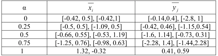
3. Numerical Example

Consider the Fuzzy Linear Complementarity Problems

( ,

q M

)

, with fuzzy triangular numbers.

Consider the fuzzy game matrices,

A =

(

) (

)

(

) (

)

90,100,110

110,160,170

130,140,190

60,110,120

⎛

⎞

⎜

⎟

⎝

⎠

and B =

(

) (

)

(

) (

)

80,105,110

110,150,190

120,140,200

80,90,140

⎛

⎞

⎜

⎟

⎝

⎠

The above fuzzy triangular number payoff matrix can be converted into the interval number payoff matrix using α-cut. The solution obtained for different α-cuts are given as follows:

α x_i

y

_j

0 [-0.42, 0.5], [-0.42,1] [-0.14,0.4], [-2.8, 1] 0.25 [-0.5, 0.5], [-1.09, 0.5] [-0.42, 0.46], [-1.15,0.54]

0.5 [-0.66, 0.55], [-0.53, 1.19] [-1.6, 1.14], [-0.73, 0.31] 0.75 [-1.25, 0.76], [-0.98, 0.63] [-2.28, 1.4], [-1.44,2.28]

1 1.32, -0.32 0.41, 0.59

4. Conclusion

variable. This method can be applied to any higher order bimatrix games. We strongly emphasize that the procedure introduced in this paper is an approximation.

REFERENCES

1. R.W.Cottle, J.S.Pang and R.E.Stone, The Linear Complementarity Problem, Republished as SIAM Classics in Applied Mathematics, Vol. 60, Philadelphia (2009).

2. V.Vijay, S.Chandra and C.R.Bector, Matrix Games with Fuzzy Goals and Fuzzy Payoffs, Omega, 33 (2005), 425-429.

3. K.G.Murthy, Linear Complementarity, Linear and Nonlinear Programming, Internet Edition, 1997.

4. A.Nagoor Gani and C.Arunkumar, A new method for solving bimatrix game using LCP under fuzzy environment, J. Math. Comput. Sci., 3(1) (2013), 135-149.

5. C.R. Bector and S. Chandra, Fuzzy Mathematical Programming and Fuzzy Matrix Games, Springer, 2005.

6. C.E.Lemke and J.T.Howson, Jr., Equilibrium points of bimatrix games, Journal of the Society for Industrial and Applied Mathematics, 12 (2) (1964), 413-423.

7. R. E. Moore, Methods and Applications of Interval Analysis, 2, SIAM Studies in Applied Mathematics, 1979.

8. S.Sohraiee, F.HosseinZadeh Lofti and M.Anisi, Two person games with interval data, Applied Mathematical Sciences, 4(28) (2010), 1355-1365.