Bounded Kernel-Based Online Learning

(1)

Bounded Kernel-Based Online Learning

∗

Francesco Orabona [email protected]

Joseph Keshet† [email protected]

Barbara Caputo [email protected]

Idiap Research Institute CH-1920 Martigny, Switzerland

Editor: Yoav Freund

Abstract

A common problem of kernel-based online algorithms, such as the kernel-based Perceptron algo-rithm, is the amount of memory required to store the online hypothesis, which may increase with-out bound as the algorithm progresses. Furthermore, the computational load of such algorithms grows linearly with the amount of memory used to store the hypothesis. To attack these problems, most previous work has focused on discarding some of the instances, in order to keep the memory bounded. In this paper we present a new algorithm, in which the instances are not discarded, but are instead projected onto the space spanned by the previous online hypothesis. We call this algorithm Projectron. While the memory size of the Projectron solution cannot be predicted before training, we prove that its solution is guaranteed to be bounded. We derive a relative mistake bound for the proposed algorithm, and deduce from it a slightly different algorithm which outperforms the Per-ceptron. We call this second algorithm Projectron++. We show that this algorithm can be extended to handle the multiclass and the structured output settings, resulting, as far as we know, in the first online bounded algorithm that can learn complex classification tasks. The method of bounding the hypothesis representation can be applied to any conservative online algorithm and to other online algorithms, as it is demonstrated for ALMA2. Experimental results on various data sets show the

empirical advantage of our technique compared to various bounded online algorithms, both in terms of memory and accuracy.

Keywords: online learning, kernel methods, support vector machines, bounded support set

1. Introduction

Kernel-based discriminative online algorithms have been shown to perform very well on binary and multiclass classification problems (see, for example, Freund and Schapire, 1999; Crammer and Singer, 2003; Kivinen et al., 2004; Crammer et al., 2006). Each of these algorithms works in rounds, where at each round a new instance is provided. On rounds where the online algorithm makes a prediction mistake or when the confidence in the prediction is not sufficient, the algorithm adds the instance to a set of stored instances, called the support set. The online classification function is defined as a weighted sum of kernel combination of the instances in the support set. It is clear that if the problem is not linearly separable or the target hypothesis is changing over time, the classification function will never stop being updated, and consequently, the support set will grow unboundedly.

∗. A preliminary version of this paper appeared in the Proceedings of the 25th International Conference on Machine Learning under the title “The Projectron: a Bounded Kernel-Based Perceptron”.

(2)

This leads, eventually, to a memory explosion, which limits the applicability of these algorithms for those tasks, such as autonomous agents, for example, where data must be acquired continuously over time.

Several authors have tried to address this problem, mainly by bounding a priori the size of the support set with a fixed value, called a budget. The first algorithm to overcome the unlimited growth of the support set was proposed by Crammer et al. (2003), and refined by Weston et al. (2005). In these algorithms, once the size of the support set reaches the budget, an instance from the support set that meets some criterion is removed, and replaced by the new instance. The strategy is purely heuristic and no mistake bound is given. A similar strategy is also used in NORMA (Kivinen et al., 2004) and SILK (Cheng et al., 2007). The very first online algorithm to have a fixed memory budget and a relative mistake bound is the Forgetron algorithm (Dekel et al., 2007). A stochastic algorithm that on average achieves similar performance to Forgetron, and with a similar mistake bound was proposed by Cesa-Bianchi et al. (2006). Unlike all previous work, the analysis presented in the last paper is within a probabilistic context, and all the bounds derived there are in expectation. A different approach to address this problem for online Gaussian processes is proposed in Csat´o and Opper (2002), where, in common with our approach, the instances are not discarded, but rather projected onto the space spanned by the instances in the support set. However, in that paper no mistake bound is derived and there is no use of the hinge loss, which often produces sparser solutions. Recent work by Langford et al. (2008) proposed a parameter that trades accuracy for sparseness in the weights of online learning algorithms. Nevertheless, this approach cannot induce sparsity in online algorithms with kernels.

In this paper we take a different route. While previous work focused on discarding some of the instances in order to keep the support set bounded, in this work the instances are not discarded. Either they are projected onto the space spanned by the support set, or they are added to the support set. By using this method, we show that the support set and, hence, the online hypothesis, is guar-anteed to be bounded, although we cannot predict its size before training. Instead of using a budget parameter, representing the maximum size of the support set, we introduce a parameter trading ac-curacy for sparseness, depending on the needs of the task at hand. The main advantage of this setup is that by using all training samples, we are able to provide an online hypothesis with high online accuracy. Empirically, as suggested by the experiments, the output hypotheses are represented with relatively small number of instances, and have high accuracy.

We start with the most simple and intuitive kernel-based algorithm, namely the kernel-based Perceptron. We modify the Perceptron algorithm so that the number of stored samples needed to represent the online hypothesis is always bounded. We call this new algorithm Projectron. The empirical performance of the Projectron algorithm is on a par with the original Perceptron algo-rithm. We present a relative mistake bound for the Projectron algorithm, and deduce from it a new online bounded algorithm which outperforms the Perceptron algorithm, but still retains all of its advantages. We call this second algorithm Projectron++. We then extend Projectron++ to the more general cases of multiclass and structured output. As far as we know, this is the first bounded mul-ticlass and structured output online algorithm, with a relative mistake bound.1 Our technique for bounding the size of the support set can be applied to any conservative kernel-based online algo-rithm and to other online algoalgo-rithms, as we demonstrate for ALMA2 (Gentile, 2001). Finally, we present some experiments with common data sets, which suggest that Projectron is comparable to

(3)

Perceptron in performance, but it uses a much smaller support set. Moreover, experiments with Pro-jectron++ shows that it outperforms all other bounded algorithms, while using the smallest support set. We also present experiments on the task of phoneme classification, which is considered to be difficult and naturally with a relatively very high number of support vectors. When comparing the Projectron++ algorithm to the Passive-Aggressive multiclass algorithm (Crammer et al., 2006), it turns out that the cumulative online error and the test error, after online-to-batch conversion, of both algorithms are comparable, although Projectron++ uses a smaller support set.

In summary, the contributions of this paper are (1) a new algorithm, called Projectron, which is derived from the kernel-based Perceptron algorithm, which empirically performs equally well, but has a bounded support set; (2) a relative mistake bound for this algorithm; (3) another algorithm, called Projectron++, based on the notion of large margin, which outperforms the Perceptron algo-rithm and the proposed Projectron algoalgo-rithm; (4) the multiclass and structured output Projectron++ online algorithm with a bounded support set; and (5) an extension of our technique to other online algorithms, exemplified in this paper for ALMA2.

The rest of the paper is organized as follows: in Section 2 we state the problem definition and the kernel-based Perceptron algorithm. Section 3 introduces Projectron, along with its theoretical analysis. Next, in Section 4 we derive Projectron++. Section 5 presents the multiclass and structured learning variant of Projectron++. In Section 6 we apply our technique for another kernel-based online algorithm, ALMA2. Section 7 describes experimental results of the algorithms presented, on different data sets. Section 8 concludes the paper with a short discussion.

2. Problem Setting and the Kernel-Based Perceptron Algorithm

The basis of our study is the well known Perceptron algorithm (Rosenblatt, 1958; Freund and Schapire, 1999). The Perceptron algorithm learns the mapping f :

X

→R based on a set of ex-amples

T

={(x1,y1),(x2,y2), . . .}, where xt ∈

X

is called an instance and yt ∈ {−1,+1}is called

a label. We denote the prediction of the Perceptron algorithm as sign(f(x))and we interpret|f(x)| as the confidence in the prediction. We call the output f of the Perceptron algorithm a

hypothe-sis, and we denote the set of all attainable hypotheses by

H

. In this paper we assume that

H

is a Reproducing Kernel Hilbert Space (RKHS) with a positive definite kernel function k :

X

×

X

→R implementing the inner producth·,·i. The inner product is defined so that it satisfies the reproducing property,hk(x,·),f(·)i= f(x).

The Perceptron algorithm is an online algorithm, where learning takes place in rounds. At each round a new hypothesis function is estimated, based on the previous one. We denote the hypothesis estimated after the t-th round by ft. The algorithm starts with the zero hypothesis, f0=0. At each round t, an instance xt∈

X

is presented to the algorithm, which predicts a label ˆyt∈ {−1,+1}using

the current function, ˆyt =sign(ft(xt)). Then, the correct label yt is revealed. If the prediction ˆyt

differs from the correct label yt, the hypothesis is updated as ft = ft−1+ytk(xt,·), otherwise the

hypothesis is left intact, ft =ft−1. The hypothesis ft can be written as a kernel expansion according

to the representer theorem (Sch¨olkopf et al., 2001),

ft(x) =

∑

xi∈St

αik(xi,x), (1)

where αi =yi and

S

t is defined to be the set of instances for which an update of the hypothesis

occurred, that is,

S

_t ={xi,0≤i≤t|yˆi6=yi}. The set

S

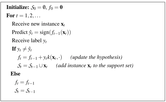
t is called the support set. The Perceptron

(4)

Initialize:

S

₀= /0, f0=0 For t=1,2, . . .

Receive new instance xt

Predict ˆyt =sign(ft−1(xt))

Receive label yt

If yt6=yˆt

ft =ft−1+ytk(xt,·) (update the hypothesis)

S

_t =

S

_t₋₁∪xt (add instance xt to the support set)

Else

ft= ft−1

S

_t =

S

_t₋₁

Figure 1: The kernel-based Perceptron Algorithm.

Although the Perceptron algorithm is very simple, it produces an online hypothesis with good performance. Our goal is to derive and analyze a new algorithm, which outputs a hypothesis that attains almost the same performance as the Perceptron hypothesis, but can be represented using many fewer instances, that is, an online hypothesis that is “close” to the Perceptron hypothesis but represented by a smaller support set. Recall that the hypothesis ft is represented as a weighted sum

over all the instances in the support set. The size of this representation is the cardinality of the support set,|

S

t|.

3. The Projectron Algorithm

This section starts by deriving the Projectron algorithm, motivated by an example of a finite dimen-sional kernel space. It continues with a description of how to calculate the projected hypothesis and describes some other computational aspects of the algorithm. The section concludes with a theoretical analysis of the algorithm.

3.1 Definition and Derivation

Let us first consider a finite dimensional RKHS

H

induced by a kernel such as the polynomial kernel. Since

H

is finite dimensional, there are a finite number of linearly independent hypotheses in this space. Hence, any hypothesis in this space can be expressed using a finite number of examples. We can modify the Perceptron algorithm to use only one set of independent instances as follows. On each round the algorithm receives an instance and predicts its label. On a prediction mistake, we check if the instance xt can be spanned by the support set, namely, for scalars di∈R,1≤i≤ |

S

t−1|, not all zeros, such that

k(xt,·) =

∑

xi∈St−1

dik(xi,·).

(5)

set. Namely, for every i

αi=yi+ytdi.

On the other hand, if the instance and the support set are linearly independent, the instance is added to the set withαt=ytas before. This technique reduces the size of the support set without changing

the hypothesis. A similar approach was used by Downs et al. (2001) to simplify SVM solutions. Let us consider now the more elaborate case of an infinite dimensional RKHS

H

induced by a kernel such as the Gaussian kernel. In this case, it is not possible to find a finite number of linearly independent vectors which span the whole space, and hence there is no guarantee that the hypothesis can be expressed by a finite number of instances. However, we can approximate the concept of linear independence with a finite number of vectors (Csat´o and Opper, 2002; Engel et al., 2004; Orabona et al., 2007).

In particular, let us assume that at round t of the algorithm there is a prediction mistake, and that the mistaken instance xt should be added to the support set,

S

t−1. Let

H

t−1be an RKHS which is the span of the kernel images of the instances in the set

S

_t₋₁. Formally,

H

t−1=span({k(x,·)|x∈

S

t−1}) . (2) Before adding the instance to the support set, we construct two hypotheses: a temporary hypothesis,

f_t′, using the function k(xt,·), that is, ft′ = ft−1+ytk(xt,·), and a projected hypothesis, ft′′, that

is the projection of f_t′ onto the space

H

_t₋₁. That is, the projected hypothesis is that hypothesis from the space

H

_t₋₁ which is the closest to the temporary hypothesis. In a later section we will describe an efficient way to calculate the projected hypothesis. Denote byδt the distance between

the hypotheses, δt = ft′′−ft′. If the norm of distance kδtk is below some threshold η, we use

the projected hypothesis as our next hypothesis, that is, ft = ft′′, otherwise we use the temporary

hypothesis as our next hypothesis, that is, ft=ft′. As we show in the following theorem, this strategy

assures that the maximum size of the support set is always finite, regardless of the dimension of the RKHS

H

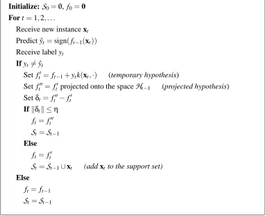
. Guided by these considerations we can design a new Perceptron-like algorithm that projects the solution onto the space spanned by the previous support vectors whenever possible. We call this algorithm Projectron. The algorithm is given in Figure 2.

The parameter η plays an important role in our algorithm. If η is equal to zero, we obtain exactly the same solution as the Perceptron algorithm. In this case, however, the Projectron solution can still be sparser when some of the instances are linearly dependent or when the kernel induces a finite dimensional RKHS

H

. Ifηis greater than zero we trade precision for sparseness. Moreover, as shown in the next section, this implies a bounded algorithmic complexity, namely, the memory and time requirements for each step are bounded. We analyze the effect ofηon the classification accuracy in Subsection 3.3.

3.2 Practical Considerations

We now consider the problem of deriving the projected hypothesis f_t′′in a Hilbert space

H

, induced by a kernel function k(·,·). Recall that f′

t is defined as ft′= ft+ytk(xt,·). Denote by Pt−1ft′ the

projection of f_t′ ∈

H

onto the subspace

H

t−1 ⊆

H

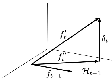
. The projected hypothesis ft′′ is defined as

f_t′′=Pt−1ft′. Schematically, this is depicted in Figure 3.

Expanding f_t′we have

(6)

Initialize:

S

₀=/0, f0=0 For t=1,2, . . .

Predict ˆyt=sign(ft−1(xt))

Receive label yt

If yt 6=yˆt

Set f_t′=ft−1+ytk(xt,·) (temporary hypothesis)

Set f_t′′= f_t′projected onto the space

H

_t₋₁ (projected hypothesis) Setδt = ft′′−ft′

Ifkδtk ≤η

ft =ft′′

S

_t =

S

_t₋₁ Else

ft =ft′

S

_t =

S

_t₋₁∪xt (add xt to the support set)

Else

ft= ft−1

S

_t=

S

_t₋₁

Figure 2: The Projectron Algorithm.

The projection is a linear operator, hence

f_t′′= ft−1+ytPt−1k(xt,·). (3)

Recall thatδt = ft′′−ft′. By substituting ft′′from Equation (3) and ft′we have

δt= ft′′−ft′=ytPt−1k(xt,·)−ytk(xt,·). (4)

The projection of f_t′∈

H

onto a subspace

H

_t₋₁⊂

H

is defined as the hypothesis in

H

_t₋₁closest to f_t′. Hence, let∑_x_j_∈St−1djk(xj,·)be an hypothesis in

H

t−1, where d= (d1, . . . ,d|St−1|)is a set of

coefficients, with di∈R. The closest hypothesis is the one for which it holds that

kδtk2=min

d

_x_j_∈

∑

St−1

djk(xj,·)−k(xt,·)

2

. (5)

Expanding Equation (5) we get

kδtk2=min

d _x

∑

i,xj∈St−1

djdik(xj,xi)−2

∑

xj∈St−1

djk(xj,xt) +k(xt,xt)

!

(7)

δ

_t

f

′′

t

f

′

t

f

t

−1

H

_t

−1

Figure 3: Geometrical interpretation of the projection of the hypothesis f_t′′onto the subspace

H

_t₋1.

Let us define Kt−1∈Rt−1×t−1to be the matrix generated by the instances in the support set

S

t−1,

that is,{Kt−1}i,j=k(xi,xj) for every xi,xj ∈

S

t−1. Let us also define kt ∈Rt−1 to be the vector

whose i-th element is kti =k(xi,xt). We have

kδtk2=min

d d

T_K

t−1d−2dTkt+k(xt,xt)

. (6)

Solving Equation (6), that is, applying the extremum conditions with respect to d, we obtain

d⋆=K_t−₋1₁kt (7)

and, by substituting Equation (7) into Equation (6),

kδtk2=k(xt,xt)−kTt d⋆. (8)

Furthermore, by substituting Equation (7) back into Equation (3) we get

f_t′′= ft−1+yt

∑

xj∈St−1

d⋆_jk(xj,·). (9)

We have shown how to calculate both the distanceδt and the projected hypothesis ft′′. In summary,

one needs to compute d⋆according to Equation (7), and plug the result either into Equation (8) to obtainδt, or into Equation (9) to obtain the projected hypothesis.

In order to make the computation more tractable, we need an efficient method to calculate the matrix inversion K−t 1iteratively. The first method, used by Cauwenberghs and Poggio (2000) for

incremental training of SVMs, directly updates the inverse matrix. An efficient way to do this, exploiting the incremental nature of the approach, is to recursively update the inverse matrix. Using the matrix inversion lemma it is possible to show (see, e.g., Csat´o and Opper, 2002) that after the addition of a new sample, K−_t 1becomes

K_t−1=



   

0

K−_t₋1₁ ... 0 0 · · · 0 0



   

+ 1 kδtk2

d⋆ −1

(8)

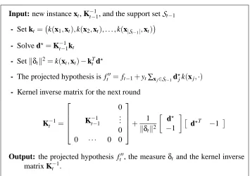
Input: new instance xt, K−t−11, and the support set

S

t−1 - Set kt= k(x1,xt),k(x2,xt), . . . ,k(x|St−1|,xt)

- Solve d⋆=K−_t₋1₁kt

- Setkδtk2=k(xt,xt)−kTt d⋆

- The projected hypothesis is f_t′′=ft−1+yt∑xj∈St−1d

⋆ jk(xj,·)

- Kernel inverse matrix for the next round

K−_t 1=



   

0

K−_t₋1₁ ... 0 0 · · · 0 0



   

+ 1 kδtk2

d⋆ −1

d⋆T −1

Output: the projected hypothesis f_t′′, the measureδt and the kernel inverse

matrix K−_t 1.

Figure 4: Calculation of the projected hypothesis f_t′′.

where d⋆ andkδtk2 are already evaluated during the previous steps of the algorithm, as given by

Equation (7) and Equation (8). Thanks to this incremental evaluation, the time complexity of the linear independence check is O(|

S

_t₋₁|2_{), as one can easily see from Equation (7). Note that the} matrix Kt−1can be safely inverted since, by incremental construction, it is always full-rank.

An alternative way to derive the inverse matrix is to use the Cholesky decomposition of Kt−1 and to update it recursively. This is known to be numerically more stable than directly updating the inverse. In our experiments, however, we found out that the method presented here is as stable as the Cholesky decomposition.

Overall, the time complexity of the algorithm is O(|

S

t|2), as described above, and the space

complexity is O(|

S

_t|2_{), due to the storage of the matrix K}−1

t , similar to the second-order Perceptron

algorithm (Cesa-Bianchi et al., 2005). A summary of the derivation of f_t′′, the projection of f_t′onto the space spanned by

S

t−1, is described in Figure 4.

3.3 Analysis

We now analyze the theoretical aspects of the proposed algorithm. First, we present a theorem which states that the size of the support set of the Projectron algorithm is bounded.

Theorem 1 Let k :

X

×

X

→Rbe a continuous Mercer kernel, with

X

a compact subset of a Banach space. Then, for any training sequence

T

={(xi,yi)},i=1,2,· · · and for anyη>0, the size of the

support set of the Projectron algorithm is finite.

(9)

an Hilbert space, k(x,x′) =hφ(x),φ(x′₎_i_and_φ_{is continuous. Given that}_φ_{is continuous and that}

_X

is compact, we obtain thatφ(

X

)is compact. From the definition ofδt in Equation (5) we get that

every time a new basis vector is added we have

η2_{≤ k}_δ

tk2=min

d

_x_j_∈

∑

St−1

djk(xj,·)−k(xt,·)

2 ≤min

dj

d_jk(x_j,·)−k(x_t,·)

2

=min

dj

d_jφ(x_j)−φ(x_t)

2 ≤

φ(x_j)−φ(x_t)

2

for any 1≤ j≤ |

S

_t₋₁|. Hence from the definition of packing numbers (Cucker and Zhou, 2007, Definition 5.17), we get that the maximum size of the support set in the Projectron algorithm is bounded by the packing number at scale η of φ(

X

). This number, in turn, is bounded by the covering number at scaleη/2, and it is finite because the set is compact (Cucker and Zhou, 2007, Proposition 5.18).

Note that this theorem guarantees that the size of the support set is bounded, however it does not state that the size of the support set is fixed or that it can be estimated before training.

The next theorem provides a mistake bound. The main idea is to bound the maximum number of mistakes of the algorithm, relative to any hypothesis g∈

H

, even chosen in hindsight. First, we define the loss with a marginγ∈Rof the hypothesis g on the example(xt,yt)as

ℓ_γ(g(xt),yt) =max{0,γ−ytg(xt)}, (10)

and we define the cumulative loss, D_γ, of g on the first T examples as

Dγ=

T

∑

t=1

ℓγ(g(xt),yt).

Before stating the bound, we present a lemma that will be used in the rest of our proofs. We will use its first statement to bound the scalar product between a projected sample and the competitor, and its second statement to derive the scalar product between the current hypothesis and the projected sample.

Lemma 2 Let(ˆx,yˆ)be an example, with ˆx∈

X

and ˆy∈ {+1,−1}. If we denote by f(·)an hypoth-esis in

H

, and denote by q(·)any function in

H

, then the following holds

ˆ

yhf,qi ≥γ−ℓ_γ(f(ˆx),yˆ)− kfk · kq−k(ˆx,·)k.

Moreover, if f(·)can be written as∑m_i₌₁αik(xi,·)withαi∈Rand xi∈

X

,i=1,· · ·,m, and q(·)is

the projection of k(ˆx,·)onto the space spanned by k(xi,·),i=1,· · ·,m, then

ˆ

yhf,qi=y fˆ (ˆx).

Proof The first inequality comes from an application of the Cauchy-Schwarz inequality and the definition of the hinge loss in Equation (10). The second equality follows from the fact thathf,q− k(ˆx,·)i=0, because f(·)is orthogonal to the difference between k(ˆx,·)and its projection onto the space in which f(·)lives.

(10)

Theorem 3 Let (x1,y1),· · ·,(xT,yT) be a sequence of instance-label pairs where xt ∈

X

, yt ∈

{−1,+1}, and k(xt,xt)≤1 for all t. Assume that the Projectron algorithm is run with η≥0.

Then the number of prediction mistakes it makes on the sequence is bounded by

kgk2 (1−ηkgk)2+

D1 1−ηkgk+

kgk 1−ηkgk

s D1 1−ηkgk

where g is an arbitrary function in

H

, such thatkgk<1

η.

Proof Define the relative progress in each round as∆t=kft−1−λgk2− kft−λgk2, whereλis a

positive scalar to be optimized. We bound the progress from above and below, as in Gentile (2003). On rounds where there is no mistake,∆t equals 0. On rounds where there is a mistake there are

two possible updates: either ft = ft−1+ytPt−1k(xt,·)or ft = ft−1+ytk(xt,·). In the following we

start bounding the progress from below, when the update is of the former type. In particular we set

q(·) =Pt−1k(xt,·)in Lemma 2 and useδt =ytPt−1k(xt,·)−ytk(xt,·)from Equation (4). Letτt be

an indicator function for a mistake on the t-th round, that is,τt is 1 if there is a mistake on round t

and 0 otherwise. We have

∆t =kft−1−λgk2− kft−λgk2=2τtythλg−ft−1,Pt−1k(xt,·)i −τt2kPt−1k(xt,·)k2

≥τt

2λ−2λℓ1(g(xt),yt)−τtkPt−1k(xt,·)k2−2λkgk · kδtk −2ytft−1(xt)

. (11)

Moreover, on every projection updatekδtk ≤η, andkPt−1k(xt,·)k ≤1 by the theorem’s assumption,

so we have

∆t≥τt

2λ−2λℓ1(g(xt),yt)−τt−2ηλkgk −2ytft−1(xt)

.

We can further bound∆t by noting that on every prediction mistake ytft−1(xt)≤0. Overall we have

kft−1−λgk2− kft−λgk2≥τt

2λ−2λℓ1(g(xt),yt)−τt−2ηλkgk

. (12)

When there is an update without projection, similar reasoning yields that

kft−1−λgk2− kft−λgk2≥τt

2λ−2λℓ1(g(xt),yt)−τt

,

hence the bound in Equation (12) holds in both cases.

We sum over t on both sides, remembering thatτt can be upper bounded by 1. The left hand

side of the equation is a telescoping sum, hence it collapses tokf0−λgk2− kfT−λgk2, which can

be upper bounded byλ2kgk2_{, using the fact that f0}₌_{0 and that}_k_f

T−λgk2is non-negative. Finally,

we have

λ2_k_g_k2₊₂_λD

1≥M(2λ−2ηλkgk −1), (13)

where M is the number of mistakes. The last equation implies a bound on M for any choice ofλ>0, hence we can take the minimum of these bounds. From now on we can suppose that M> D1

1−ηkgk.

In fact, if M≤ D1

1−ηkgk then the theorem trivially holds. The minimum of Equation (13) as a function

ofλoccurs at

(11)

By our hypothesis that M> D1

1−ηkgk we have thatλ∗is positive. Substitutingλ∗into Equation (13)

we obtain

(D1−M(1−ηkgk))2

kgk2 −M≤0. Solving for M and overapproximating concludes the proof.

This theorem suggests that the performance of the Projectron algorithm is slightly worse than that of the Perceptron algorithm. Specifically, if we setη=0, we recover the best known bound for the Perceptron algorithm (see for example Gentile, 2003). Hence the degradation in the performance of Projectron compared to Perceptron is related to₁₋_η1_k_g_k. Empirically, the Projectron algorithm and the Perceptron algorithm perform similarly, for a wide range of settings ofη.

4. The Projectron++ Algorithm

The proof of Theorem 3 suggests how to improve the Projectron algorithm to improve upon the performance of the Perceptron algorithm, while maintaining a bounded support set. We can change the Projectron algorithm so that an update takes place not only if there is a prediction mistake, but also when the confidence of the prediction is low. We refer to this latter case as a margin error, that is, 0<ytft−1(xt)<1. This strategy is known to improve the classification rate but also increases

the size of the support set (Crammer et al., 2006). A possible solution to this obstacle is not to update on every round in which a margin error occurs, but only when there is a margin error and the new instance can be projected onto the support set. Hence, the update on round in which there is a margin error would in general be of the form

ft= ft−1+ytτtPt−1k(xt,·),

with 0<τt≤1. The last constraint comes from the proof of Theorem 3, where we upper boundτt

by 1. Note that settingτt to 0 is equivalent to leaving the hypothesis unchanged.

In particular, disregarding the loss term in Equation (11), the progress∆t can be made positive

with an appropriate choice ofτt. Whenever this progress is non-negative the worst-case number

of mistakes decreases, hopefully along with the classification error rate of the algorithm. With this modification we expect better performance, that is, fewer mistakes, but without any increase of the support set size. We can even expect solutions with a smaller support set, since new instances can be added to the support set only if misclassified, hence having fewer mistakes should result in a smaller support set. We name this algorithm Projectron++. The following theorem states a mistake bound for Projectron++, and guides us in how to chooseτt.

X

, yt ∈

{−1,+1}, and k(xt,xt)≤1 for all t. Assume that Projectron++ is run with η>0. Then the

number of prediction mistakes it makes on the sequence is bounded by

kgk2 (1−ηkgk)2+

D1 1−ηkgk+

kgk 1−ηkgk

s

max

0, D1

1−ηkgk−B

(12)

H

, such thatkgk<1

η,

0<τt <min

 



2ℓ1(ft−1(xt),yt)−

kδtk

η

kPt−1k(xt,·)k2 ,1

 



and

B=

∑

{t:0<ytft−1(xt)<1}

τt

2ℓ1(ft−1(xt),yt)−τtkPt−1k(xt,·)k2−2

kδtk

η

>0.

Proof The proof is similar to the proof of Theorem 3, where the difference is that during rounds in which there is a margin error we update the solution whenever it is possible to project ensuring an improvement of the mistake bound. Assume thatλ≥1. On rounds when a margin error occurs, as in Equation (11), we can write

∆t+2τtλℓ1(g(xt),yt)≥ τt 2λ−τtkPt−1k(xt,·)k2−2λkδtk · kgk −2ytft−1(xt)

> τt

2

1−kδtk η

−τtkPt−1k(xt,·)k2−2ytft−1(xt)

= τt

2ℓ1(ft−1(xt),yt)−τtkPt−1k(xt,·)k2−2

kδtk

η

, (14)

where we used the bounds onkgkandλ. Letβt be the right hand-side of Equation (14). A sufficient

condition to haveβt positive is

τt <2

ℓ1(ft−1(xt),yt)−kδ_ηtk

kPt−1k(xt,·)k2 .

Constrainingτt to be less than or equal to 1 yields the update rule in the theorem.

Let B=∑_{_t:0_<_y_t_f_t₋₁₍_x_t₎_<₁_}βt. Similarly to the proof of Theorem 3, we have

λ2_k_g_k2₊₂_λD

1≥M(2λ−2ηλkgk −1) +B. (15) Again, the optimal value ofλis

λ∗₌M(1−ηkgk)−D1 kgk2 . We can assume that M(1−ηkgk)−D1≥ kgk2. In fact, if M<kgk

2₊_D 1

1−ηkgk, then the theorem trivially

holds. With this assumption, λ∗ is positive and greater than or equal to 1, satisfying our initial constraint onλ. Substituting this optimal value ofλinto Equation (15), we have

(D1−M(1−ηkgk))2

(13)

The proof technique presented here is very general, in particular it can be applied to the Passive-Aggressive algorithm PA-I (Crammer et al., 2006). In fact, removing the projection step and up-dating on rounds in which there is a margin error, with ft = ft−1+ytτtk(xt,·), we end up with the

condition 0<τt <min

n

2ℓ1(ft−1(xt),yt)

kk(xt,·)k2 ,1

o

. This rule generalizes the PA-I bound whenever R=1 and C=1, however the obtained bound substantially improves upon the original bound in Crammer et al. (2006).

The theorem gives us some freedom for the choice ofτt. Experimentally we have observed that

we obtain the best performance if the update is done with the following rule

τt =min

 



ℓ1(ft−1(xt),yt)

kPt−1k(xt,·)k2

,2ℓ1(ft−1(xt),yt)−

kδtk

η

 



.

The added term in the minimum comes from ignoring the term−2kδtk

η and in finding the maximum

of the quadratic equation. Notice that the termkPt−1k(xt,·)k2in the last equation can be practically

computed as kT_t d⋆, as can be derived using the same techniques presented in Subsection 3.2. We note in passing that the condition on whether xt can be projected onto

H

t−1on margin error may stated asℓ1(ft−1(xt),yt)≥kδ_ηtk. This means that if the loss is relatively large, the progress is

also large and the algorithm can afford “wasting” a bit of it for the sake of projecting.

The algorithm is summarized in Figure 2. The performance of the Projectron++ algorithm, the Projectron algorithm and several other bounded online algorithms are compared and reported in Section 7.

5. Extension to Multiclass and Structured Output

In this section we extend Projectron++ to the multiclass and the structured output settings (note that Projectron can be generalized in a similar way). We start by presenting the more complex decision problem, namely the structured output, and then we derive the multiclass decision problem as a special case.

In structured output decision problems the set of possible labels has a unique and defined struc-ture, such as a tree, a graph or a sequence (Collins, 2000; Taskar et al., 2003; Tsochantaridis et al., 2004). Denote the set of all labels as

Y

={1, . . . ,k}. Each instance is associated with a label from

Y

. Generally, in structured output problems there may be dependencies between the instance and the label, as well as between labels. Hence, to capture these dependencies, the input and the output pairs are represented in a common feature representation. The learning task is therefore defined as finding a function f :

X

×

Y

→_Rsuch that

yt =arg max

y∈Y f(xt,y). (16)

Let us generalize the definition of the RKHS

H

introduced in Section 2 to the case of structured learning. A kernel function in this setting should reflect the dependencies between the instances and the labels, hence we define the structured kernel function as a function on the domain of the instances and the labels, namely, kS_:₍

_X

_×

_Y

₎2 _→_R_{. This kernel function induces the RKHS}

H

S_{, where the inner product in this space is defined such that it satisfies the reproducing property,}

(14)

Initialize:

S

₀=/0, f0=0 For t=1,2, . . .

Predict ˆyt=sign(ft−1(xt))

Receive label yt

If yt 6=yˆt (prediction error)

Set f_t′= ft−1+ytk(xt,·)

Set f_t′′=Pt−1ft′

Setδt= ft′′−ft′

Ifkδtk ≤η

ft = ft′′

S

_t =

S

_t₋₁ Else

ft = ft′

S

_t =

S

_t₋₁∪xt

Else If yt=yˆtand ytft−1(xt)≤1 (margin error)

Setδt=Pt−1k(xt,·)−k(xt,·)

Ifℓ1(ft−1(xt),yt)≥kδ_ηtk (check if the xt can be projected onto

H

t−1)

Setτt =min

ℓ1(ft−1(xt),yt)

kPt−1k(xt,·)k2,2

ℓ1(ft−1(xt),yt)−kδ_ηtk

Set ft = ft−1+ytτtPt−1k(xt,·)

S

_t =

S

_t₋₁ Else

ft = ft−1

S

_t =

S

_t₋₁ Else

ft =ft−1

S

_t =

S

_t₋₁

Figure 5: The Projectron++ Algorithm.

As in the binary classification algorithm presented earlier, the structured output online algorithm receives instances in a sequential order. Upon receiving an instance, xt∈

X

, the algorithm predicts a

label, y′_t, according to Equation (16). After making its prediction, the algorithm receives the correct label, yt. We define the loss suffered by the algorithm on round t for the example(xt,yt)as

ℓS_γ(f,xt,yt) =max{0,γ−f(xt,yt) +max y′t6=yt

(15)

and the cumulative loss DS_γ as

DS_γ =

T

∑

t=1

ℓS

γ(f,xt,yt).

Note that sometimes it is useful to defineγas a functionγ:

Y

×

Y

→Rdescribing the discrepancy between the predicted label and the true label. Our algorithm can handle such a label cost function, but we will not discuss this issue here (see Crammer et al., 2006, for further details).

As in the binary case, on rounds in which there is a prediction mistake, y′_t 6=yt, the algorithm

updates the hypothesis ft−1 by adding k((xt,yt),·)−k((xt,y′t),·)or its projection. When there is

a margin mistake, 0< ℓS

γ(ft−1,xt,yt)<γ, the algorithm updates the hypothesis ft−1 by adding

τtPt−1(k((xt,yt),·)−k((xt,y′t),·)), where 0<τt<1 and will be defined shortly. Now, for the

struc-tured output case,δt is defined as

δt =k((xt,yt),·)−k((xt,y′t),·)−Pt−1 k((xt,yt),·)−k((xt,y′t),·)

.

The analysis of the structured output Projectron++ algorithm is similar to that provided for the binary case. We can easily obtain the generalization of Lemma 2 and Theorem 4 as follows

Lemma 5 Let(ˆx,yˆ)be an example, with ˆx∈

X

and ˆy∈

Y

. Denote by f(·)an hypothesis in

H

S_.

Let q(·)∈

H

S_{. Then the following holds for any y}′_∈

_Y

_:

hf,qi ≥γ−ℓS_γ(f,ˆx,yˆ)− kfk ·q− k((ˆx,yˆ),·)−k((ˆx,y′),·)

.

Moreover if f(·)can be written as∑m_i₌₁αik((xi,yi),·)withαi∈Rand xi∈

X

,i=1,· · ·,m, and q is

the projection of k((ˆx,yˆ),·)−k((ˆx,y′),·)in the space spanned by k((xi,yi),·),i=1,· · ·,m, we have

that

hf,qi= f(ˆx,yˆ)−f(ˆx,y′).

Theorem 6 Let(x1,y1),· · ·,(xT,yT)be a sequence of instance-label pairs where xt ∈

X

, yt ∈

Y

,

andkk((xt,y),·)k ≤1/2 for all t and y∈

Y

. Assuming that Projectron++ is run withη>0, the

kgk2 (1−ηkgk)2+

DS₁

1−ηkgk+ kgk 1−ηkgk

s

max

0, D S

1

1−ηkgk−B

H

S_{, such that}_k_g_k_< 1

η,

a = Pt−1 k((xt,yt),·)−k((xt,y′t),·)

0<τt < min

 



2ℓ

S

1(ft−1,xt,yt)−kδ_ηtk

kak2 ,1

 



B =

∑

{t:0<ℓS

1(ft−1,xt,yt)<1}

τt

2ℓS₁(ft−1,xt,yt)−τtkak2−2

kδtk

η

(16)

As in Theorem 4 there is some freedom in the choice ofτt, and again we set it to

τt =min







ℓS

1(ft−1,xt,yt)

kak2 ,2

ℓS

1(ft−1,xt,yt)−kδ_ηtk

kak2 ,1







.

In the multiclass decision problem case, the kernel k((x1,y1),(x2,y2)) is simplified to

δy1y2k(x1,x2), where δy1y2 is the Kronecker delta. This corresponds to the use of a different

pro-totype for each class. This simplifies the projection step, in fact k((xt,yt),·)can be projected only

onto the functions in St−1 belonging to yt, the scalar product with the other functions being zero.

So instead of storing a single matrix K_t−₋1₁, we need to store m matrices, where m is the number of classes, each one being the inverse matrix of the Gram matrix of the functions of one class. This results in improvements in both memory usage and computational cost of the algorithm. To see this suppose that we have m classes, each with n vectors in the support set. Storing a single matrix means having a space and time complexity of O(m2n2)(cf. Section 3), while in the second case the complexity is O(mn2). We use this method in the multiclass experiments presented in Section 7.

6. Bounding Other Online Algorithms

It is possible to apply the technique in the basis of the Projectron algorithm to any conservative online algorithm. A conservative online algorithm is an algorithm that updates its hypothesis only on rounds on which it makes a prediction error. By applying Lemma 2 to a conservative algorithm, we can construct a bounded version of it with worst case mistake bounds. As in the previous proofs, the idea is to use Lemma 2 to bound the scalar product of the competitor and the projected function. This yields an additional term which is subtracted from the marginγof the competitor.

The technique presented here can be applied to other online kernel-based algorithms. As an example, we apply our technique to ALMA2 (Gentile, 2001). Again we define two hypotheses: a temporary hypothesis f_t′, which is the hypothesis of ALMA2after its update rule, and a projected hypothesis, which is the hypothesis f_t′ projected on the set

H

_t₋₁as defined in Equation (2). Define the projection errorδt asδt= ft′−ft′′. The modified ALMA2algorithm uses the projected

hypoth-esis f_t′′whenever the projection error is smaller than a parameterη, otherwise it uses the temporary hypothesis f_t′. We can state the following bound

X

, yt ∈

{−1,+1}, and k(xt,xt)≤1 for all t. Letα, B and C∈R+satisfy the equation

C2+2(1−α)BC=1.

Assume ALMA2(α;B,C) projects every time the projection errorkδtkis less than η≥0, then the

Dγ

γ−η+ ρ2

2 +

s ρ4

4 +

ρ2

γ−ηDγ+ρ2 whereγ>η,ρ= 1

C2₍_γ₋_η₎2, and g is an arbitrary function in

H

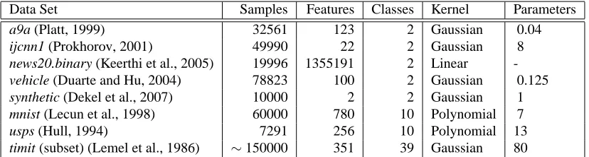
, such thatkgk ≤1.

(17)

Data Set Samples Features Classes Kernel Parameters

a9a (Platt, 1999) 32561 123 2 Gaussian 0.04

ijcnn1 (Prokhorov, 2001) 49990 22 2 Gaussian 8

news20.binary (Keerthi et al., 2005) 19996 1355191 2 Linear -vehicle (Duarte and Hu, 2004) 78823 100 2 Gaussian 0.125 synthetic (Dekel et al., 2007) 10000 2 2 Gaussian 1 mnist (Lecun et al., 1998) 60000 780 10 Polynomial 7

usps (Hull, 1994) 7291 256 10 Polynomial 13

timit (subset) (Lemel et al., 1986) ∼150000 351 39 Gaussian 80

Table 1: Data sets used in the experiments

γ−η−ℓ_γ(g(xt),yt), and further substituteγ−ηforγ.

7. Experimental Results

In this section we present experimental results that demonstrate the effectiveness of the Projec-tron and the ProjecProjec-tron++ algorithms. We compare both algorithms to the PercepProjec-tron algorithm, the Forgetron algorithm (Dekel et al., 2007) and the Randomized Budget Perceptron (RBP) algo-rithm (Cesa-Bianchi et al., 2006). For Forgetron, we choose the state-of-the-art “self-tuned” variant, which outperforms all of its other variants. We used the PA-I variant of the Passive-Aggressive algo-rithm (Crammer et al., 2006) as a baseline algoalgo-rithm, as it gives an upper bound on the classification performance of the Projectron++ algorithm. All the algorithms were implemented in MATLAB us-ing the DOGMA library (Orabona, 2009).

We tested the algorithms on several standard machine learning data sets:2a9a, ijcnn1, news20.binary, vehicle (combined), usps, mnist. We also used a synthetic dataset and the acoustic-phonetic dataset timit. The synthetic dataset was built in the same way as in Dekel et al. (2007). It is composed of

10000 samples taken from two separate bi-dimensional Gaussian distributions. The means of the positive and negative samples are(1,1)and(−1,−1), respectively, while the covariance matrices for both are diagonal matrices with(0.2,2) as their diagonal. The labels are flipped with a proba-bility of 0.1 to introduce noise. The list of the data sets, their characteristics and the kernels used, are given in Table 1. The parameters of the kernels were selected to have the best performance with the Perceptron and were used for all the other algorithms to result in a fair comparison. The

C parameter of PA-I was set to 1, to give an update similar to Perceptron and Projectron. All the

experiments were performed over five different permutations of the training set.

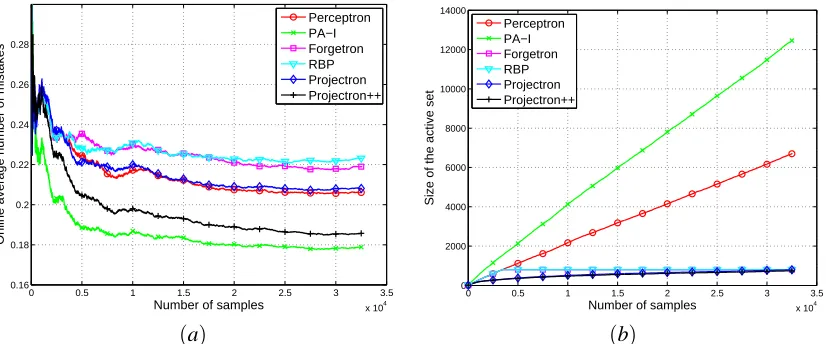
Experiments with one setting of η. In the first set of experiments we compared the online average number of mistakes and the support set size of all algorithms. Both Forgetron and RBP work by discarding vectors from the support set, if the size of the support set reaches the budget size, B. Hence for a fair comparison, we set η to some value and selected the budget sizes of Forgetron and RBP to be equal to the final size of the support set of Projectron. In particular, in Figure 6, we setη=0.1 in Projectron and ended up with a support set of size 793, hence B=793. In Figure 6(a) the average online error rate for all algorithms on the a9a data set is plotted. Note that Projectron closely tracks Perceptron. On the other hand Forgetron and RBP stop improving

(18)

0 0.5 1 1.5 2 2.5 3 3.5 x 104 0.16

0.18 0.2 0.22 0.24 0.26 0.28

Number of samples

Online average number of mistakes

Perceptron PA−I Forgetron RBP Projectron Projectron++

0 0.5 1 1.5 2 2.5 3 3.5 x 104 0

2000 4000 6000 8000 10000 12000 14000

Number of samples

Size of the active set

(a) (b)

Figure 6: Average online error (left) and size of the support set (right) for the different algorithms on a9a data set as a function of the number of training samples (better viewed in color).

B is set to 793,η=0.1.

after reaching the support set size B, around 3400 samples. Moreover, as predicted by its theoretical analysis, Projectron++ achieves better results than Perceptron, even with fewer number of supports. Figure 6(b) shows the growth of the support set as a function of the number of samples. While for the PA-I and the Perceptron the growth is clearly linear, it is sub-linear for Projectron and Pro-jectron++: they will reach a maximum size and then they will stop growing, as stated in Theorem 1. Another important consideration is that Projectron++ outperforms Projectron both with respect to the size of the support set and number of mistakes. Using our MATLAB implementation, the run-ning times for this experiment are∼35s for RBP and Forgetron,∼40s for Projectron and Projec-tron++, ∼130s for Perceptron, and ∼375s for PA-I. Hence Projectron and Projectron++ have a running time smaller than Perceptron and PA-I, due to their smaller support sets.

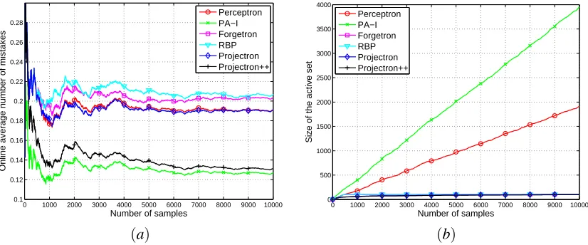
The same behavior can be seen in Figure 7, for the synthetic data set. Here the gain in perfor-mance of Projectron++ over Perceptron, Forgetron and RBP is even greater.

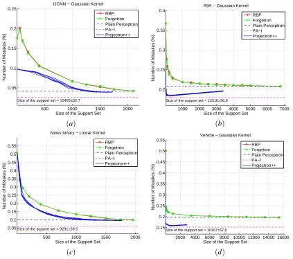
Experiments with a range of values forη- Binary. To analyze in more detail the behavior of our algorithms we decided to run other tests using a range of values ofη. For each value we obtain a different size of the support set and a different number of mistakes. We used the data to plot a curve corresponding to the percentage of mistakes as a function of the support set size. The same curve was plotted for Forgetron and RBP, where the budget size was selected as described before. In this way we compared the algorithms along the continuous range of budget sizes, displaying the trade-off between sparseness and accuracy. For the remaining experiments we chose not to show the performance of Projectron, as it was always outperformed by Projectron++.

(19)

0 1000 2000 3000 4000 5000 6000 7000 8000 9000 10000 0.1

0.12 0.14 0.16 0.18 0.2 0.22 0.24 0.26 0.28

Number of samples

Online average number of mistakes

0 1000 2000 3000 4000 5000 6000 7000 8000 9000 10000 0

500 1000 1500 2000 2500 3000 3500 4000

Number of samples

Size of the active set

(a) (b)

Figure 7: Average online error (left) and size of the support set (right) for the different algorithms on the synthetic data set as a function of the number of training samples (better viewed in color). B is set to 103,η=0.04.

note that there is a point in all the graphs where the performance of Projectron++ is better than Perceptron, and has a smaller support set. Projectron++ gets closer to the classification rate of the PA-I, without paying the price of a larger support set. Note that the performance of Projectron++ is consistently better than RBP and Forgetron, regardless of the kernel used, particularly, on the database news20.binary, which is a text classification task with linear kernel. In this task the samples are almost mutually orthogonal, so finding a suitable subspace on which to project is difficult. Nevertheless Projectron++ succeeded in obtaining better performance. The reason is probably due to the margin updates, which are performed without increasing the size of the solution. Note that a similar modification would not be trivial in Forgetron and in RBP, because the proofs of their mistake bounds strongly depend on the rate of growth of the norm of the solution.

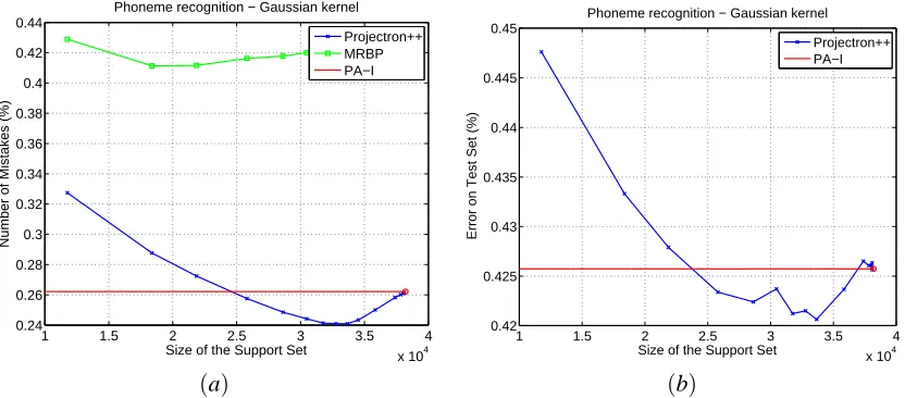
Experiments with a range of values forη- Multiclass. We have also considered multiclass data sets, using the multiclass version of Projectron++. Due to the fact that there are no other bounded online algorithms with a mistake bound for multiclass, we have extended RBP in the natural manner to multiclass. In particular we used the max-score update in Crammer and Singer (2003), for which a mistake bound exists, discarding a vector at random from the solution each time a new instance is added and the number of support vectors is equal to the budget size. We name it Multiclass Random Budget Perceptron (MRBP). It should be possible to prove a mistake bound for this algorithm, extending the proof in Cesa-Bianchi et al. (2006). In Figure 9 we show the results for Perceptron, Passive-Aggressive, Projectron++ and MRBP trained on (a) usps, and (b) mnist data sets. The results confirm the findings found for the binary case.

(20)

500 1000 1500 2000 0.05 0.1 0.15 0.2 0.25

IJCNN − Gaussian Kernel

Size of the Support Set

Number of Mistakes (%)

Size of the support set = 10493±52.7

RBP Forgetron Plain Perceptron PA−I Projectron++

1000 2000 3000 4000 5000 6000 7000 0.2

0.25 0.3 0.35 0.4

A9A − Gaussian Kernel

(a) (b)

500 1000 1500 2000 0.05 0.1 0.15 0.2 0.25 0.3 0.35 0.4 0.45 0.5 0.55

News binary − Linear Kernel

2000 4000 6000 8000 10000 12000 14000 16000 0.15 0.2 0.25 0.3 0.35 0.4 0.45 0.5 0.55

Vehicle − Gaussian Kernel

(c) (d)

Figure 8: Average online error for the different algorithms as a function of the size of the support set on different binary data sets.

(21)

100 200 300 400 500 0

0.1 0.2 0.3 0.4 0.5

USPS − Polynomial Kernel

MRBP Plain Perceptron PA−I Projectron++

500 1000 1500 2000 2500 0

0.1 0.2 0.3 0.4 0.5

MNIST − Polynomial Kernel

MRBP Plain Perceptron PA−I Projectron++

(a) (b)

Figure 9: Average online error for the different algorithms as a function of the size of the support set on different multiclass data sets.

1 1.5 2 2.5 3 3.5 4 x 104 0.24

0.26 0.28 0.3 0.32 0.34 0.36 0.38 0.4 0.42 0.44

Phoneme recognition − Gaussian kernel Projectron++ MRBP PA−I

1 1.5 2 2.5 3 3.5 4 x 104 0.42

0.425 0.43 0.435 0.44 0.445 0.45

Error on Test Set (%)

Phoneme recognition − Gaussian kernel Projectron++ PA−I

(a) (b)

Figure 10: Average online error(a) and test error(b) for the different algorithms as a function of the size of the support set on a subset of the timit data set.

8. Discussion

(22)

before training, practically, for a given target accuracy, the size of the support sets of Projectron or Projectron++ are much smaller than those of other budget algorithms such as Forgetron and RBP.

The first algorithm, Projectron, is based on the Perceptron algorithm. The empirical perfor-mance of Projectron is comparable to that of Perceptron, but with the advantage of a bounded solution. The second algorithm, Projectron++, introduces the notion of large margin and, for some values of η, outperforms the Perceptron algorithm, while assuring a bounded solution. The ex-perimental results suggest that Projectron++ outperforms other online bounded algorithms such as Forgetron and RBP, with a similar hypothesis size.

There are two unique advantages of Projectron and Projectron++. First, these algorithms can be extended to the multiclass and the structured output settings. Second, a standard online-to-batch conversion can be applied to the online bounded solution of these algorithms, resulting in a bounded batch solution. The major drawback of these algorithms is their time and space complexity, which is quadratic in the size of the support set. Trying to overcome this acute problem is left for future work.

Acknowledgments

The authors would like to thank the anonymous reviewers for suggesting a way to improve Theorem 3. This work was supported by EU project DIRAC (FP6-0027787). The authors would like to thank Andy Cotter for proofreading the manuscript.

References

G. Cauwenberghs and T. Poggio. Incremental and decremental support vector machine learning. In

Advances in Neural Information Processing Systems 14, pages 409–415, 2000.

N. Cesa-Bianchi, A. Conconi, and C. Gentile. On the generalization ability of on-line learning algorithms. IEEE Trans. on Information Theory, 50(9):2050–2057, 2004.

N. Cesa-Bianchi, A. Conconi, and C. Gentile. A second-order perceptron algorithm. SIAM Journal

on Computing, 34(3):640–668, 2005.

N. Cesa-Bianchi, A. Conconi, and C. Gentile. Tracking the best hyperplane with a simple budget Perceptron. In Proc. of the 19th Conference on Learning Theory, pages 483–498, 2006.

L. Cheng, S. V. N. Vishwanathan, D. Schuurmans, S. Wang, and T. Caelli. Implicit online learning with kernels. In Advances in Neural Information Processing Systems 19, pages 249–256, 2007.

M. Collins. Discriminative reranking for natural language parsing. In Proc. of the 17th International

Conference on Machine Learning, pages 175–182, 2000.

K. Crammer and Y. Singer. Ultraconservative online algorithms for multiclass problems. Journal

of Machine Learning Research, 3:951–991, 2003.

K. Crammer, J. Kandola, and Y. Singer. Online classification on a budget. In Advances in Neural

(23)

K. Crammer, O. Dekel, J. Keshet, S. Shalev-Shwartz, and Y. Singer. Online passive-aggressive algorithms. Journal of Machine Learning Research, 7:551–585, 2006.

L. Csat´o and M. Opper. Sparse on-line gaussian processes. Neural Computation, 14:641–668, 2002.

F. Cucker and D. X. Zhou. Learning Theory: An Approximation Theory Viewpoint. Cambridge University Press, New York, NY, USA, 2007.

O. Dekel, S. Shalev-Shwartz, and Y. Singer. The Forgetron: A kernel-based perceptron on a budget.

SIAM Journal on Computing, 37(5):1342–1372, 2007.

T. Downs, K. E. Gates, and A. Masters. Exact simplification of support vectors solutions. Journal

of Machine Learning Research, 2:293–297, 2001.

M. F. Duarte and Y. H. Hu. Vehicle classification in distributed sensor networks. Journal of Parallel

and Distributed Computing, 64:826–838, 2004.

Y. Engel, S. Mannor, and R. Meir. The kernel recursive least-squares algorithm. IEEE Transactions

on Signal Processing, 52(8):2275–2285, 2004.

Y. Freund and R. E. Schapire. Large margin classification using the Perceptron algorithm. Machine

Learning, pages 277–296, 1999.

C. Gentile. A new approximate maximal margin classification algorithm. Journal of Machine

Learning Research, 2:213–242, 2001.

C. Gentile. The robustness of the p-norm algorithms. Machine Learning, 53(3):265–299, 2003.

J. J. Hull. A database for handwritten text recognition research. IEEE Transactions on Pattern

Analysis and Machine Intelligence, 16(5):550–554, 1994.

S. S. Keerthi, D. Decoste, and T. Joachims. A modified finite newton method for fast solution of large scale linear svms. Journal of Machine Learning Research, 6:2005, 2005.

J. Kivinen, A. Smola, and R. Williamson. Online learning with kernels. IEEE Trans. on Signal

Processing, 52(8):2165–2176, 2004.

J. Langford, L. Li, and T. Zhang. Sparse online learning via truncated gradient. In Advances in

Neural Information Processing Systems 21, pages 905–912, 2008.

Y. Lecun, L. Bottou, Y. Bengio, and P. Haffner. Gradient-based learning applied to document recognition. Proceedings of the IEEE, 86(11):2278–2324, November 1998.

L. Lemel, R. Kassel, and S. Seneff. Speech database development: Design and analysis. Report no. SAIC-86/1546, Proc. DARPA Speech Recognition Workshop, 1986.

F. Orabona. DOGMA: A MATLAB Toolbox for Online Learning, 2009. Software available athttp: //dogma.sourceforge.net.

(24)

J. C. Platt. Fast training of support vector machines using sequential minimal optimization. In B. Sch¨olkopf, C. Burges, and A. Smola, editors, Advances in kernel methods – support vector

learning, pages 185–208. MIT Press, Cambridge, MA, USA, 1999.

D. Prokhorov. IJCNN 2001 neural network competition. Technical report, 2001.

F. Rosenblatt. The Perceptron: A probabilistic model for information storage and organization in the brain. Psychological Review, 65:386–407, 1958.

B. Sch¨olkopf, R. Herbrich, and A. J. Smola. A generalized representer theorem. In Proc. of the 14th

Conference on Computational Learning Theory, pages 416–426, London, UK, 2001.

Springer-Verlag.

B. Taskar, C. Guestrin, and D. Koller. Max-margin Markov networks. In Advances in Neural

Information Processing Systems 17, 2003.

I. Tsochantaridis, T. Hofmann, T. Joachims, and Y. Altun. Support vector machine learning for interdependent and structured output spaces. In Proc. of the 21st International Conference on

Machine Learning, pages 823–830, 2004.