The University of San Francisco
USF Scholarship: a digital repository @ Gleeson Library |
Geschke Center
Master's Theses Theses, Dissertations, Capstones and Projects
Spring 5-16-2014
Heterogeneous Effects of Commodity Price
Shocks on Inflation Rates. Evidence from a Panel
Study.
Odbayar Batmunkh
University of San Francisco, [email protected]
Follow this and additional works at:https://repository.usfca.edu/thes
Part of theInternational Economics Commons
This Thesis is brought to you for free and open access by the Theses, Dissertations, Capstones and Projects at USF Scholarship: a digital repository @ Gleeson Library | Geschke Center. It has been accepted for inclusion in Master's Theses by an authorized administrator of USF Scholarship: a digital repository @ Gleeson Library | Geschke Center. For more information, please [email protected].
Recommended Citation
Batmunkh, Odbayar, "Heterogeneous Effects of Commodity Price Shocks on Inflation Rates. Evidence from a Panel Study." (2014). Master's Theses. 84.
Heterogeneous Effects of Commodity Price Shocks on
Inflation Rates. Evidence from a Panel Study.
Master’s Thesis
International and Development Economics
Key Words: Commodity prices, Exports, Imports, Inflation
Odbayar Batmunkh
e-mail: [email protected]
May 2014
Abstract: Do commodity price shocks have heterogeneous effect on countries based on their export and import profiles? I address this question through a panel study of 142 countries using Export and Import Indexes aimed at differentiating the retail pass-through and fiscal balance channel of transmission of Commodity Price shocks on inflation. The results show that an increase in the Export Index leads to a decrease in contemporary inflation while an increase in the Import Index leads to an increase in inflation in the next year. Average causal mediating effect of the Export Index on Inflation through the Fiscal Balance was shown to be negative.*
I would like to thank Professors Man Chiu (Sunny) Wong and Jacques Artus for their guidance and mentorship in this research project.
1. Introduction
Inflation plays a big role in the lives of the poor around the world. The poor have limited access to banking services, this leaves them unable to offset their losses to inflation. Beck (2007) has found that people in the Least Developed Countries (LDCs) have significantly lower access to banking services than people in Developed Countries. The recent episode of hyperinflation in Zimbabwe ,as analyzed by Coomer (2011), is the most outrageous example of government mismanagement of the money supply. Wines (2006) reports anecdotal evidence of negative impacts on the residents of Zimbabwe. However one does not have to experience hyperinflation to incur losses to welfare from inflation. Fujii (2013) found evidence that the poor are especially vulnerable to inflation and especially food inflation. Easterly (2001) found in an extensive survey that the poor name inflation as their top economic concern. Cardoso (1992) argues that the poor in Latin American countries are not affected by inflation because their cash holdings are too small.
In 2011 atleast 25 countries in the world experience double digit inflation according to the World Bank and all of those countries are in the Developing World. This causes the poor to lose purchasing power or change their purchasing decisions to offset inflation. The poor, in the absence of banking services, may choose to buy consumer durables to offset inflation. Even this move will still net them a loss in welfare as the consumer durable good earns a negative return equal to its depreciation. Easterly (2001) found that inflation reduced the real wage of the poor and states that inflation is a “cruel tax” on the poor.
The earliest look at inflation was done by Phillips (1958) who found a relationship between inflation and unemployment in the United States between 1861 and 1958. This finding was embraced by the Keynesian economists of the early half of the 20th century. However the hyperinflation of the 1970s in the United States and the complete breakdown of the Phillips curve in empirical testing after 1960s opened the door for the Quantity Theory of Money. Gali (1999) and other economists are still trying to revive the idea of the Phillips curve.
The dominant theory on inflation today considers it as purely a monetary phenomenon. This theory is based on the Quantity Theory of Money and was brought back to attention by Friedman (1953). This theory says that the only determinants of the inflation rate are the relative supply of money and goods in the economy. Friedman also suggested a constant money supply growth rule to help combat inflation.
was the cause of this drop in inflation around the world. Alesina and Summers (1993) believed it was the heterogeneity in central bank independence that could explain this sudden change. Romer (1993) and Lane (1997) argued that increased openness of the economy also increased the cost of unexpected inflation and therefore reduced the temptation to engage in excessive money supply increases. The famous Lucas (1976) critique of backward looking economic models created a new paradigm in economic models of inflation.
With the introduction of forward-looking expectations money supply alone cannot be sufficient in explaining the inflation dynamics of many countries. To this line of thought Sargent and Wallace (1981) predicted that the ability of the monetary policy to target inflation may only be effective with coordination with fiscal side of economic policy. Sargent and Wallace (1981) predicted that tight monetary policy could lead to a higher inflation rate under certain conditions. With a given demand for government bonds and no changes in future fiscal policy some of the debt has to be inflated away using seigniorage.
Related to Sargent and Wallace (1981) is the Fiscal Theory of the Price Level, which was developed by Leeper (1991), Sims (1994) and Woodford (1994). The Fiscal Theory of the Price Level argues that an increase in government deficits has an effect on the price level. Empirical work in Catao (2005) showed a strong association between deficits and inflation among high inflation developing countries.
Inflation plays a big role in the decision making function of households, individuals and companies. One such example is the impact of inflation in lowering real wages and reducing rigidity in wages of labor markets. Wage rigidity was shown to be nominal in nature and only reduced by inflation. Nominal inflation was shows not to decrease even in times of drought. Thus workers were unwilling to accept lower wages even in tough times. (Kaur 2012) Therefore inflation serves a very important function in reducing unemployment during
recessions. Inflation was shows to “ grease the wheels” of labor markets as predicted by Tobin (1972). One way through which inflation influences the decision making of poor individuals could be the propagation effect of price shocks in a specific product group. Propagation happens when a price hike in one product group also affects the prices in other product groups. Pedersen (2010) found that price shocks in food products resulted in higher propagation than price shocks in energy products, also emerging countries are more affected by propagation than advanced.
printing a new menu or the cost of changing the price of the firm’s product in every outlet. This cost has an effect on the firm’s decision to change the price of its product based on the increase in underlying costs. Therefore firms may or may not shift the higher cost to consumers based on the degree of price increase. There is extensive literature in microeconomics that looks at the ways that companies shift the increasing costs of raw commodities to the
customers, which results in inflation. This argument was extended by Christiano et al. (2005) who looked at the impact of expansionary monetary policy shock on marginal output.
Christiano et al.(2005) determined that staggered wage contracts and variable capital utilization impacted the degree to which inflation expectations were driving changes in real marginal costs. Rigobon (2010) used micro price data to test how much of the underlying raw material cost increases was passed on to customers. Rigobon (2010) found that sectors responded differently across countries and commodities. Therefore different characteristics of each sector have an impact on the pass through of commodity price shocks.
Exporting countries may be affected differently by a rise in underlying costs compared to net raw commodity importers. This may not be a simple case of higher raw inputs leading to higher inflation for every country. Zoli (2009) found that international commodity price shocks have a significant impact on domestic inflation, however the effect of commodity price shocks was asymmetric to inflation in a panel of 18 European countries. Previous studies of
commodity prices looked at the retail pass-through channel and assumed homogeneous effects on inflation and could not reach a consensus. Awokuse and Yang (2002), Cutler et
al.(2005) and Jumah and Kunst (2007) found that commodity prices do affect inflation while Blomberg and Harris (1995), and Furlong and Ingenito (1996) found that commodity prices do not affect inflation.
Previous work on commodity prices focused on growth rates Deaton (1999) and the Resource Curse Auty (1993). My approach also differs from existing literature on budget deficits and inflation (Elmendorf,1993; Catao and Terrones, 2005) by introducing
heterogeneous effects of commodity price shocks on inflation and budget deficits through the Export Index and the Import Index approach. The intuition behind this approach is that a rise in the price of a certain commodity will only have an effect on the country's inflation rate if the country exports or imports that commodity.
year through the retail pass-through channel. The effect of the Export Index varies by the country's income group level and by the level of inflation in the country.
Following this introduction, Section 2 of my paper presents a description of the methodology and the econometrics model used in this paper. Section 3 describes the data used in this paper. Section 4 presents the results and Section 5 summarizes and concludes.
2. Methodology
2.1 Commodity Price Index
At the core of my approach is the Commodity Price Index. In this paper I am following the methodology first used by Deaton (1999). I construct a country specific commodity Export and Import Price Index that captures exogenous shocks to commodity prices :
CommodityIndexi,t = ∏cϵC ComPricec,tθi,c
where ComPricec,t is the price of commodity c in year t. θi,cis the average export or import
weight assigned to each commodity. These weights are based on the time invariant value of exports or imports of a commodity in the GDP of the country i. This functional form of the commodity price index follows common practice in the literature, for example Collier(2007). Using this approach I can create a unique index that captures the relative value of Exports or Imports to each country. This allows me to introduce heterogeneous effects to the underlying changes in global commodity prices by differentiating between the retail pass-through channel of import commodity prices and the impact of export commodity prices on the inflation rate. I used time invariant weights to get around the limitations of the data and also to establish a unique profile of a country that is based on the average amount of a commodity
exported/imported as a share of GDP over 30 years. I created the index using local currency and US dollars to test if the variation in the Index is coming from price changes in the underlying commodities or changes in the exchange rate. Following Deaton (1999) the
commodities in question are aluminum, beef, coffee, cocoa, copper, cotton, gold, iron, maize, oil, rice, rubber, sugar, tea, tobacco, wheat and wood.
2.2 Estimation Strategy
∆logCPIi,t=γ1∆ logCPIi,t-1+γ2 ∆logExportIndexi,t+γ3 ∆logExportIndexi,t-1 +γ4 ∆logImportIndexi,t+γ5 ∆logImportIndexi,t-1 +γ6 ∆logManufacturedIndext +γ7∆ logManufacturedIndext-1 + γ8∆ logExchangeRatei,t + γ9∆ logM2i,t + γ10 ∆logM2i,t-1
+γ11∆logGDPGapi,t +αi +βt + μi,t
In the above equation the inflation rate of a country is defined as the log change in CPI. α
i are country fixed effects that capture time invariant country specific unobserved variables and
βt are year fixed effects that capture common year shocks. μi,t is the error term clustered at the country level. I use the change of the log of the Export/Import Indexes to ensure that within-country variations in the Export/Import Indexes are due to percentage changes in the local currency commodity prices. Manufactured Goods Index is a measurement of the import price of manufactured goods and is calculated in US dollars. GDP Gap , M2 , Exchange Rate , CPI and the Export/Import Indexes are calculated in local currency.
In the baseline regression I estimate the average marginal effect of commodity price fluctuations on CPI inflation by using the largest possible sample size. Later I split up the sample by income groups and level of inflation to test for heterogeneity in the marginal effects.
3. Data:
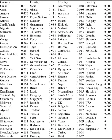
Data on annual international commodity prices for the 1970-2009 period was obtained from UNCTAD Commodity Statistics (UNCTAD,2009). Data on the value of Commodity Exports and Imports is from NBER-United Nations Trade Database (Feenstra et al., 2004). Commodities used in the index are aluminum, beef, coffee, cocoa, copper, cotton, gold, iron, maize, oil, rice, rubber, sugar, tea, tobacco, wheat and wood. For some commodities multiple prices were listed, I used a simple average of those prices. Data on the price of iron was not available for 2010-2013 years, this reduced my sample time frame to 1970-2009. Additionally the data on commodity Exports/Imports had multiple entries for some commodities, only the category describing raw commodities was used. The methodology by Deaton (1999) called for using the average time invariant weights, this helped overcome some missing data problems in the value of Exports/Imports database. NBER-United Nations Trade Database does not report zero values, thus one cannot differentiate between missing values and 0 commodities
highest weights in the sample, while a developed country like the United States has weights close to 0.
Macroeconomic data is mostly from the International Financial Statistics (IFS) database of the IMF. Additionally data from World Bank's World Development Indicators was used. The data set covers 142 countries and up to 38 annual observations per country. The definition of money supply is M2. Fiscal Balance data is from Catao (2005). Fiscal Balance data from the IMF only included deficit data from the central government and did not include state or local governments. Using more comprehensive data from Catao (2005) increased my Fiscal Balance observations from 1400 to 2800.
4. Results:
3.1 Main results
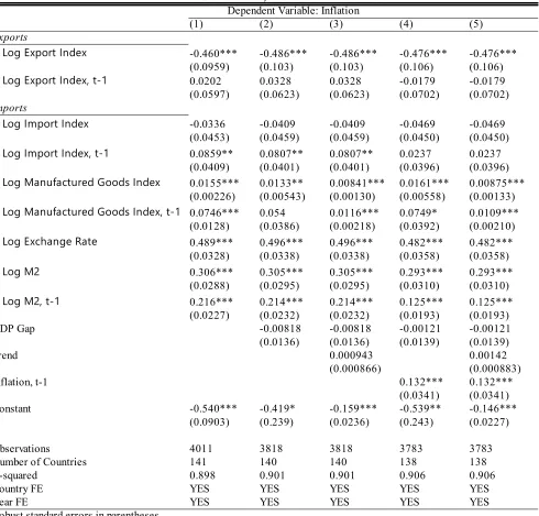
Table 3 shows the main results. In this table all variables are in log changes and local currency, except for the Manufactured Goods index which is in US dollars. The coefficients on the Manufactured Goods Index and the first lag of the Manufactured Goods Index is positive and significant at 1%. This suggests that an increase in the cost of manufactured goods leads to an increase in inflation. This finding is consistent with economic theory and expectations. The coefficient on the Exchange Rate is positive and significant, this suggests that an increase in the Exchange Rate is associated with an increase in the inflation rate. This is consistent with economic theory and is significant with the addition of other covariates. The changes in M2 is correlated with an increase in the inflation rate in both contemporary and next years. This result confirms the monetary theory of the money supply as the main driver of inflation. The first lag of the inflation rate is added to capture any possible omitted variables, this follows the methodology of Kwon (2008).
The coefficient on the log of the Export Index is negative in the contemporary case and is not significant in the first lag. This suggests that an increase in the Export Commodity Index is associated with a reduction in the inflation rate in the current year. This result suggests that the Price of Exported Commodities affects inflation differently from the Price of Imported Commodities. The coefficient is negative and significant at 1% level even with the addition of covariates.
Commodity Prices on inflation in a country. This result also confirms heterogeneous effect of commodity prices on inflation based on the Export/Import profile of that country. However this result is not significant when the first lag of the inflation rate is added in column 4 and 5. The regressions in Table 3 have between 4011 and 3783 observations with the number of countries ranging from 141 to 138. Country fixed effects and year fixed effects have been used to test for country specific and year specific shocks to inflation. The high R-squared suggests that the model is properly specified. Additionally the time trend was introduced to capture and reduction in global inflation due to the time trend.
Table 4 uses the Export and Import Indexes in US dollar currency to test whether the results in Table 3 come from changes in the underlying price of the commodities or the change in the relative Exchange Rates of each country. The coefficients on the Export Index are similar and significant at 1% level. The different size of the coefficient can be explained by the different base of the US Dollar and the Local Currency Indexes. The coefficient on the Import Index is significant only at the 10% level now, before the inclusion of the first lag of inflation.
Table 5 breaks down the sample into four different income groups based on the classification by the World Bank. The local currency Export Index has a negative coefficient in Lower Income , Middle Income and High Income OECD countries, but is not significant in the High Income non OECD group. This suggests that Low and Middle Income countries experienced reduction in their inflation rates when their Export Index increased. However this effect disappears in the High Income non OECD case. This can be explained by the make of countries in the High Income non OECD group, which consists mostly of wealthy oil exporting countries in the Middle East, Russia and are known for their weak institutional quality.
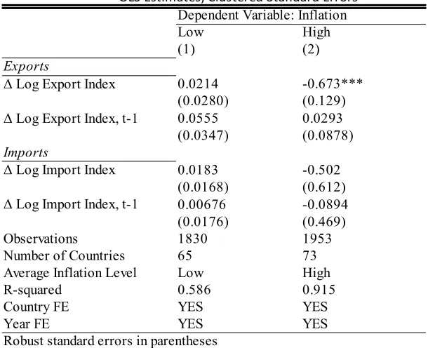
Table 7 breaks down the sample by their inflation rates. The results show that countries with highest observed inflation rates experience the largest effects of Export Index on inflation. This is consistent with the deficit channel of mediation, as theory suggests that countries that have large and chronic deficits experience high inflation. Countries that generally have low levels of inflation they are not likely to be affected by the Export Index. The coefficient of the Export Index in column 4 and 5 differ greatly in size. This suggests that most of the result comes from countries that have large and chronic deficits, which improve their Fiscal Balance by using commodity Export revenue.
countries that export raw commodities do not have enough market power to influence the price of a commodity. Figure 1 shows a diagram of the Fiscal Balance channel and explains how an exogenous change in the price of an export commodity can lead to an increase in the Fiscal Balance of a country. An improvement in the Fiscal Balance of a country then reduces inflation as shown by Catao (2005). Column 1 of Table 6 shows that an improvement in the Fiscal Balance leads to a reduction in the inflation rate in the current year. Column 2 of Table 6 shows that an exogenous increase in the Export Index leads to an improvement in the Fiscal Balance.
Using methodology by Imai (2011) in American Political Science Review the Average Causal
Mediating Effect (ACME) was calculated using the coefficient multiplication approach. Assuming Sequential Ignorability and No-Interaction assumptions ACME is asymptotically consistent and equal to -0.02. Figure 2 shows that ACME is negative and significant at the ρ=0. Sequential Ignorability is a valid assumption in the Fiscal Balance channel as all arrows point outward from the Fiscal Balance except for the Export Index.
5. Summary and Conclusions
References
Alesina, A., & Tabellini, G. (1989). External debt, capital flight and political risk. Journal of International Economics, 27(3), 199-220.
Alesina, A., & Summers, L. H. (1993). Central bank independence and macroeconomic
performance: some comparative evidence. Journal of Money, Credit and Banking, 25(2), 151-162.
Arezki, R., & Brückner, M. (2012). Commodity Windfalls, Democracy and External Debt*. The Economic Journal, 122(561), 848-866.
Auty, Richard M. "Industrial policy reform in six large newly industrializing countries: The resource curse thesis." World development 22.1 (1994): 11-26.
Awokuse, Titus O., and Jian Yang. "The informational role of commodity prices in formulating monetary policy: a reexamination." Economics Letters 79.2 (2003): 219-224.
Barton, J., 2009. The Chilean Case. In Rhys Jenkins & Enrique Dussel Peters, eds., 2009. China and Latin America: Economic Relations in the Twenty-first Century. Bonn & Mexico City: Deutsches Institut für Entwicklungspolitik &
Universidad Nacional Autónoma de México.
Beck, T., Demirguc-Kunt, A., & Martinez Peria, M. S. (2007). Reaching out: Access to and use of banking services across countries. Journal of Financial Economics, 85(1), 234-266. Bloomberg, S. Brock and Harris, ìThe Commodity ñ Consumer Price Connection: Fact
or Fable?," Federal Reserve Bank of New York Economic Policy Review, October, 1995, pages 21 - 38.
Buiter, Willem H., 1999, “The Fallacy of the Fiscal Theory of the Price Level,” NBER Working Paper No. 7302 (Cambridge, Massachusetts: National Bureau of Economic Research).
Caldentey, Esteban Pérez, and Matías Vernengo. "Back to the future: Latin America's current development strategy." Journal of Post Keynesian Economics 32.4 (2010): 623-644.
Catao, L., and M. Terrones, 2005, “Fiscal Deficits and Inflation,” Journal of Monetary Economics, Vol. 52, pp. 529–54.
Cardoso, E. (1992). Inflation and poverty (No. w4006). National Bureau of Economic Research.
Christiano, Lawrence J., Martin Eichenbaum, and Charles L. Evans. "Nominal rigidities and the dynamic effects of a shock to monetary policy." Journal of political Economy 113.1 (2005): -45.
Coomer, J., & Gstraunthaler, T. (2011). The Hyperinflation in Zimbabwe. Quarterly Journal Of Austrian Economics, 14(3), 311-346.
Deaton, Angus. "Commodity prices and growth in Africa." The Journal of Economic Perspectives (1999): 23-40.
Desormeaux, Jorge, Pablo García, and Claudio Soto. Terms of trade, commodity prices and inflation dynamics in Chile. Banco Central de Chile, 2009.
Easterly, W., & Fischer, S. (2001). Inflation and the Poor. Journal of Money, Credit and Banking, 160-178.
Elmendorf, Douglas W., 1993, “Actual Budget Deficit Expectations and Interest Rates,” Harvard Institute of Economic Research, Discussion Paper No. 1639.
Fischer, Stanley, R. Sahay, and C. Vegh, 2002, “Modern Hyper- and High inflations,” Journal of Economic Literature, Vol. 40, No. 3 (September), pp. 837–80.
Friedman, M. (1956), “The Quantity Theory of Money: A Restatement” in Studies in the Quantity Theory of Money, edited by M. Friedman.
Fujii, T. (2013). Impact of Food Inflation on Poverty in the Philippines. Food Policy, 3913-27.
Furlong, Fred, and Robert Ingenito. "Commodity prices and inflation."Economic Review-Federal Reserve Bank of San Francisco (1996): 27-47.
Hogenboom, B., 2010. The Return of the State in Latin America’s Mineral Policies: And What about Civil Society?. Paper presented for the ECPR workshop Towards Strong Publics? Civil Society and the State in Latin America, Münster, Germany, 23-25 March, 2010.
Imai, Kosuke, Luke Keele, and Teppei Yamamoto. "Identification, inference and sensitivity analysis for causal mediation effects." Statistical Science 25.1 (2010): 51-71.
Imai, Kosuke, et al. "Unpacking the black box of causality: Learning about causal mechanisms from experimental and observational studies." American Political Science Review 105.4 (2011): 765-789.
Jaggers, K., & Marshall, M. G. (2009). Polity IV Project: Dataset Users’ Manual. Center for Systemic Peace.
Jumah, Adusei, and Robert M. Kunst. "Seasonal prediction of European cereal prices: good forecasts using bad models?." Journal of Forecasting 27.5 (2008): 391-406.
Galı, J., & Gertler, M. (1999). Inflation dynamics: A structural econometric analysis. Journal of monetary Economics, 44(2), 195-222.
Kirby, P., 2010. Globalisation and State-Civil Society Relations: Lessons from Latin America. Paper prepared for the ECPR workshop Towards Strong Publics? Civil Society and the State in Latin America, Münster, Germany, 23-25 March, 2010.
Kaur, Supreet. 2012. “Nominal Wage Rigidity in Village Labor Markets.” Mimeo, Harvard University.
Kwon, G., McFarlane, L., & Robinson, W. (2006). Public debt, money supply, and inflation: A cross-country study and its application to Jamaica.
Lane, P. R. (1997). Inflation in open economies. Journal of International Economics, 42(3-4), 327-347.
Mankiw, N. Gregory. "Small menu costs and large business cycles: A macroeconomic model of monopoly." The Quarterly Journal of Economics100.2 (1985): 529-537.
McCallum, B. T., & Nelson, E. (1999). Nominal income targeting in an open-economy optimizing model. Journal of Monetary economics, 43(3), 553-578.
Leeper, E. M. (1991). Equilibria under ‘active’and ‘passive’monetary and fiscal policies. Journal of monetary Economics, 27(1), 129-147.
López, Ramón, and Sebastian J. Miller. "Chile: the unbearable burden of inequality." World Development 36.12 (2008): 2679-2695.
Lucas, R. E. (1976, January). Econometric policy evaluation: A critique. In Carnegie-Rochester conference series on public policy (Vol. 1, No. 1, pp. 19-46).
Persson, T. and Tabellini, G. (1998), Political economics and macroeconomic policy,
in J. B. Taylor and M. Woodford, eds, `Handbook of Macroeconomics', Vol. 1C, North Holland, Amsterdam, chapter 22.
Pedersen, M. (2010), “Propagation of inflationary shocks in Chile and an international comparison of propagation of shocks to food and energy prices”, Working Paper No. 566, Central Bank of Chile.
Persson, T., Tabellini, G., & Trebbi, F. (2003). Electoral rules and corruption. journal of the European Economic Association, 1(4), 958-989.
Phillips, A. W. (1958). The Relation Between Unemployment and the Rate of Change of Money Wage Rates in the United Kingdom, 1861–19571. economica, 25(100), 283-299.
Reinhart, C. M., & Rogoff, K. S. (2010). Growth in a Time of Debt (No. w15639). National Bureau of Economic Research.
Rigobon, R., 2010, “Commodity prices pass-through”, Working Paper No. 572, Central Bank of Chile.
Romer, D. (1993). Openness and inflation: theory and evidence. The Quarterly Journal of Economics, 108(4), 869-903.
Sargent, T. J., & Wallace, N. (1981). Some unpleasant monetarist arithmetic. Federal Reserve Bank of Minneapolis Quarterly Review, 5(3), 1-17.
Silva P. (1991): “Technocrats and politics in Chile: from the Chicago Boys to the CIEPLAN Monks”, Journal of Latin American Studies, 23 (2), pp. 385-410.
Silva P. (2008): In the name of reason. Technocrats and politics in Chile, The Pennsylvania State University Press, Pennsylvania.
Sims, C. A. (1994). A simple model for study of the determination of the price level and the interaction of monetary and fiscal policy. Economic Theory, 4(3), 381-399.
Singh, Anoop, Agnes Belaisch, Charles Collyns, Paula De Masi, Reva Krieger, Guy Meredith, and Robert Rennhack, 2005, Stabilization and Reform in Latin America: a
Singh, Jewellord T. Nem. "Governing the Extractive Sector: The Politics of Globalisation and Copper Policy in Chile." Journal of Critical Globalisation Studies 3 (2010).
Solimano, Andrés. Chile and the neoliberal trap: the post-Pinochet era. Cambridge University Press, 2012.
Taylor, J. B. (1993, December). Discretion versus policy rules in practice. In Carnegie-Rochester conference series on public policy (Vol. 39, pp. 195-214). North-Holland.
Tobin, James. "Inflation and unemployment." American Economic Review 62.1 (1972): 1-18.
Tornell, A., & Lane, P. R. (1999). The voracity effect. American Economic Review, 22-46.
Van der Ploeg, F. (2011). Natural resources: Curse or blessing?. Journal of Economic Literature,
49(2), 366-420.
Wines, M. (2006). How bad is inflation in Zimbabwe?. New York Times, 2.
Woodford, M., 1994, “Monetary Policy and Price Level Determined in a Cash-in-Advance Economy,” Economic Theory, Vol. 4, pp. 345–80.
Figure 1: Exports Affect Inflation Through the Fiscal Balance Channel
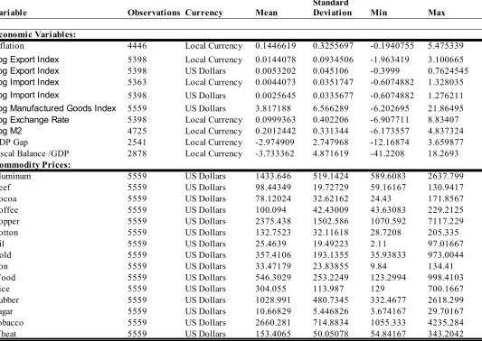
Variable Observations Currency Mean Min Max
Economic Variables:
Inflation 4446 Local Currency 0.1446619 0.3255697 -0.1940755 5.475339
5398 Local Currency 0.0144078 0.0934506 -1.963419 3.100665
5398 US Dollars 0.0053202 0.045106 -0.3999 0.7624545
5363 Local Currency 0.0044073 0.0351747 -0.6074882 1.328035
5398 US Dollars 0.0025645 0.0335677 -0.6074882 1.276211
5559 US Dollars 3.817188 6.566289 -6.202695 21.86495
5398 Local Currency 0.0999363 0.402206 -6.907711 8.83407
Log M2 4725 Local Currency 0.2012442 0.331344 -6.173557 4.837324
GDP Gap 2541 Local Currency -2.974909 2.747968 -12.16874 3.659877
Fiscal Balance /GDP 2878 Local Currency -3.733362 4.871619 -41.2208 18.2693
Commodity Prices:
Aluminum 5559 US Dollars 1433.646 519.1424 589.6083 2637.799
Beef 5559 US Dollars 98.44349 19.72729 59.16167 130.9417
Cocoa 5559 US Dollars 78.12024 32.62162 24.43 171.8567
Coffee 5559 US Dollars 100.094 42.43009 43.63083 229.2125
Copper 5559 US Dollars 2375.438 1502.586 1070.592 7117.229
Cotton 5559 US Dollars 132.7523 32.11618 28.7208 205.335
Oil 5559 US Dollars 25.4639 19.49223 2.11 97.01667
Gold 5559 US Dollars 357.4106 193.1355 35.93833 973.0044
Iron 5559 US Dollars 33.47179 23.83855 9.84 134.41
Wood 5559 US Dollars 546.3029 253.2249 123.2994 998.4103
Rice 5559 US Dollars 304.055 113.987 129 700.1667
Rubber 5559 US Dollars 1028.991 480.7345 332.4677 2618.299
Sugar 5559 US Dollars 10.66829 5.446826 3.674167 29.70167
Tobacco 5559 US Dollars 2660.281 714.8834 1055.333 4235.284
Wheat 5559 US Dollars 153.4065 50.05078 54.84167 343.2042
Table 1: Summary Statistics
Standard Deviation
Log Export Index Log Export Index Log Import Index LogImport Index
Country Country Country Country
Oman 0.6 Syria 0.111 Azerbaijan 0.038 Lithuania 0.007 Qatar 0.587 Ghana 0.111 Sudan 0.036 Poland 0.007 Angola 0.475 Uganda 0.111 Australia 0.034 Bahamas 0.006 Guyana 0.454 Papua N.Guin 0.11 Mexico 0.034 Malta 0.006 Kuwait 0.446 Ecuador 0.089 Ireland 0.033 Hungary 0.006 Saudi Arabia 0.445 Guatemala 0.086 Ethiopia 0.029 India 0.005 Nigeria 0.369 Seychelles 0.085 Malawi 0.023 Gambia 0.005 Suriname 0.356 Tajikistan 0.084 New Zealand 0.023 Finland 0.005 Iraq 0.345 Honduras 0.084 Philippines 0.023 Croatia 0.005 Congo 0.342 Egypt 0.084 Pakistan 0.022 Slovenia 0.005 Gabon 0.342 Costa Rica 0.081 Burkina Faso 0.022 Senegal 0.004 St.Kt-Nev-An 0.288 Togo 0.08 Bolivia 0.021 Romania 0.004 Zambia 0.284 Burundi 0.078 Cambodia 0.021 Mongolia 0.004 Untd Arab Em 0.28 Norway 0.074 Brazil 0.02 Israel 0.004 Liberia 0.27 Viet Nam 0.072 Ukraine 0.02 Switz.Liecht 0.004 Libya 0.267 Dominican Rp 0.071 Canada 0.02 Albania 0.004 Yemen 0.259 GuineaBissau 0.07 Zimbabwe 0.019 Nepal 0.004 Eq.Guinea 0.239 Colombia 0.068 Kyrgyzstan 0.019 Czech Rep 0.003 Iran 0.231 Chad 0.061 Sri Lanka 0.019 Djibouti 0.003 Cote Divoire 0.194 Cent.Afr.Rep 0.057 Estonia 0.018 Jordan 0.003 Guinea 0.164 Mali 0.053 Panama 0.017 Sweden 0.003 Mauritius 0.161 Sierra Leone 0.051 Niger 0.016 Bosnia Herzg 0.003 Belize 0.155 Benin 0.051 Bahrain 0.016 Korea Rep. 0.003 Kazakhstan 0.145 Latvia 0.05 Mozambique 0.015 Slovakia 0.003 Trinidad Tbg 0.144 Paraguay 0.05 South Africa 0.014 Armenia 0.003 Cameroon 0.144 Singapore 0.048 Netherlands 0.014 Belarus 0.002 Malaysia 0.143 Rwanda 0.048 UK 0.014 USA 0.002 Venezuela 0.141 Kenya 0.046 Bulgaria 0.013 Cyprus 0.002 Algeria 0.14 Thailand 0.046 Samoa 0.012 Italy 0.001 Fiji 0.131 Tunisia 0.044 Argentina 0.011 Morocco 0.001 Jamaica 0.13 Peru 0.043 Georgia 0.011 Lebanon 0 El Salvador 0.121 Madagascar 0.043 China 0.009 Iceland 0 Nicaragua 0.119 Barbados 0.043 Denmark 0.009 Japan 0 Indonesia 0.117 Russian Fed 0.042 Lao P.Dem.R 0.008 Bangladesh 0 Dem.Rp.Congo 0.115 Tanzania 0.04 Turkey 0.008
Mauritania 0.111 Uruguay 0.04 Haiti 0.007
Local Currency Index
---OLS Estimates, Clustered Standard
Errors---Dependent Variable: Inflation
(1) (2) (3) (4) (5)
Exports
-0.460*** -0.486*** -0.486*** -0.476*** -0.476*** (0.0959) (0.103) (0.103) (0.106) (0.106) 0.0202 0.0328 0.0328 -0.0179 -0.0179 (0.0597) (0.0623) (0.0623) (0.0702) (0.0702) Imports
-0.0336 -0.0409 -0.0409 -0.0469 -0.0469 (0.0453) (0.0459) (0.0459) (0.0450) (0.0450) 0.0859** 0.0807** 0.0807** 0.0237 0.0237 (0.0409) (0.0401) (0.0401) (0.0396) (0.0396) 0.0155*** 0.0133** 0.00841*** 0.0161*** 0.00875*** (0.00226) (0.00543) (0.00130) (0.00558) (0.00133) 0.0746*** 0.054 0.0116*** 0.0749* 0.0109*** (0.0128) (0.0386) (0.00218) (0.0392) (0.00210) 0.489*** 0.496*** 0.496*** 0.482*** 0.482*** (0.0328) (0.0338) (0.0338) (0.0358) (0.0358) 0.306*** 0.305*** 0.305*** 0.293*** 0.293*** (0.0288) (0.0295) (0.0295) (0.0310) (0.0310) 0.216*** 0.214*** 0.214*** 0.125*** 0.125*** (0.0227) (0.0232) (0.0232) (0.0193) (0.0193)
GDP Gap -0.00818 -0.00818 -0.00121 -0.00121
(0.0136) (0.0136) (0.0139) (0.0139)
Trend 0.000943 0.00142
(0.000866) (0.000883)
Inflation, t-1 0.132*** 0.132***
(0.0341) (0.0341)
Constant -0.540*** -0.419* -0.159*** -0.539** -0.146***
(0.0903) (0.239) (0.0236) (0.243) (0.0227)
Observations 4011 3818 3818 3783 3783
Number of Countries 141 140 140 138 138
R-squared 0.898 0.901 0.901 0.906 0.906
Country FE YES YES YES YES YES
Year FE YES YES YES YES YES
Robust standard errors in parentheses *** p<0.01, ** p<0.05, * p<0.1
Table 3. Effect of Commodity Price Shocks on Inflation
Δ Log Export Index
Δ Log Export Index, t-1
Δ Log Import Index
Δ Log Import Index, t-1
Δ Log Manufactured Goods Index
Δ Log Manufactured Goods Index, t-1
Δ Log Exchange Rate
Δ Log M2
Table 6. Fiscal Balance Channel of Mediation
Local Currency Index
---OLS Estimates, Clustered Standard
Errors---Dependent Variable: Inflation Dependent Variable: Fiscal Balance
(1) (2) Exports -0.566** 11.78*** (0.266) (3.171) -0.16 (0.115) Imports -0.05 (0.0374) 0.00474 (0.0339) 0.0144** (0.00656) -0.00109 (0.00313) -0.00201** (0.000815) 0.508*** -3.214*** (0.0388) (0.570) 0.331*** (0.0435) 0.120*** (0.0249)
GDP Gap -0.00543
(0.00689)
Trend 0.00485*
(0.00277)
Inflation, t-1 0.101**
(0.0398)
Constant -0.155** -3.192***
(0.0778) (0.563)
Observations 2087 2801
Number of Countries 84 96
R-squared 0.939 0.418
Country FE YES YES
Year FE YES YES
Robust standard errors in parentheses *** p<0.01, ** p<0.05, * p<0.1
Δ Log Export Index
Δ Log Export Index, t-1
Δ Log Import Index
Δ Log Import Index, t-1
Δ Log Manufactured Goods Index
Δ Log Manufactured Goods Index, t-1
Δ Fiscal Balance
Δ Log Exchange Rate
Δ Log M2
Local Currency Index
---OLS Estimates, Clustered Standard
Errors---Dependent Variable: Inflation
Low High
(1) (2)
Exports
0.0214 -0.673*** (0.0280) (0.129)
0.0555 0.0293
(0.0347) (0.0878) Imports
0.0183 -0.502
(0.0168) (0.612) 0.00676 -0.0894 (0.0176) (0.469)
Observations 1830 1953
Number of Countries 65 73
Average Inflation Level Low High
R-squared 0.586 0.915
Country FE YES YES
Year FE YES YES
Robust standard errors in parentheses *** p<0.01, ** p<0.05, * p<0.1
Table 7. Effect of Commodity Price Shocks on Inflation
Δ Log Export Index
Δ Log Export Index, t-1
Δ Log Import Index
Appendix
My study looks at the impact of commodity prices changes on the inflation rates of a panel of 140 countries. This Appendix focuses on a single country, Chile, and for this reason is qualitative in nature. This case study will focus on the two driving narratives of Chile's economic history in the last 40 years, “super cycle” in the price of copper and elite capture. Chile has been the exception to the global failure of “neoliberal” economic policies around the world. This exceptionalism was shaped by limited political diversity, protection of the “neoliberal” model from criticism at the cost of equality and individual rights. These policies contributed to Chile's high per capita income growth in the past 40 years. The 2008 financial crisis and the perceived failure of laissez-faire financial reforms in the United States, the cradle of neoliberal policies, shook the public's faith in “free market” capitalism domestically and also globally. This was the impetus for a host of social movements in Chile aimed to challenge the past neoliberal policies.
A.1 Introduction to Chile
Chile is located in South America and stretches along the western coast of the continent from Peru to the southernmost tip of South America. Chile is a mountainous country with large supplies of natural-resources and natural ports on its western coast that enabled its colonization by European settlers. The most abundant natural-resource of Chile are its copper reserves, that are mostly located in the northern Atacama Desert. A second notable resource of Chile is wine that is grown in the Central Valley of Chile, located in the middle of the country.
Copper exports play a huge role in Chile, accounting for half of all exports in 2010. The copper export sector is dominated by international firms which pay royalty and taxes on their earnings. The state copper exporter CODELCO was downsized as part of the neoliberal policy of privatization. This means that majority of the profits from copper exports accrue to foreign firms. The copper export sector does not create any jobs downstream from it, because it is a raw commodity exporter. Most of the supplies for the copper export sector are provided by foreign firms and mostly comprise machinery. The sustainability of this finite natural resource exporting strategy is questionable. For this reason Chile ranks poorly in most indexes that cover Environmental Sustainability.
The modern Chilean political narrative begins with the election of Eduardo Frei Montalva of the “Christian Democrats” in 1964. This centrist candidate started policies to nationalize the mostly United States owned copper companies, agrarian reform and overall progressive social policies. During this time all of South America was under the influence of socialist rhetoric from the Soviet Union and this mobilized the peasants, urban residents , students and labor activists to create the alliance of socialists, Unidad Popular. Their candidate in the 1970 election was Salvador Allende. Upon election Allende embarked on a policy of “Chilean socialism” aimed to nationalize large industry and especially the copper industry. Allende's policy of nationalism and fiscal expansion was financed by seigniorage and resulted in high inflation. These movements were perceived by the United States government and wealthy Chileans as paving the way for a socialist country. With the country embargoed by the United States and dissatisfaction with the new policies high at home, Chile was prime for a coup to swing the pendulum to the other extreme of the political spectrum.
Pinochet was the chief of the armed forces when he overthrew Allende on September 11 1973. Acting on a perceived Soviet threat to Chile , Pinochet enacted a policy of brutal crackdown on any forms of dissent to his rule. Scores of opposition activists were abducted and murdered by the Chilean military and secret police.
To implement economic reform Pinochet turned to the United States and the University of Chicago in particular. 25 Chilean nationals trained at the University of Chicago were
aggregate consumption and aggregate investment. The 1982 financial crisis and the ensuing recession combined to decrease real wages , increase poverty and unemployment in the country.
The government's reaction was to drop the fixed exchange rate of the Chilean peso versus the US dollar on recommendation from Milton Friedman. This increased the public debt of the country overnight and negatively affected companies that borrowed in US dollars. The overall cost to the Chilean government of the 1982 financial crisis was roughly 40% of the GDP.
For his sins Pinochet was never indicted or jailed. He was placed under house arrest in 1998 on a visit to the United Kingdom. Later Pinochet was extradited back to Chile where was intermittently under house arrest but was not indicted for any crimes during his presidency. Aside from being inconvenienced Pinochet escaped justice and died in 2006 a free man. The decision not to charge Pinochet in Chile for his crimes illustrates the power of Pinochet's powerbase and the complicity of those currently in power in the same crimes.
In the 1988 a referendum was called to decide whether Pinochet could serve another 8 year term as president. Upon Pinochet's defeat Chile was now on a path to democracy. The first freely elected president was Patricio Aylwin from the Christian Democrat party. The transition from military dictatorship to democracy rested on the guarantee that neoliberal economic policy would be sustained and those responsible for the crackdown and repression would not be prosecuted. The new government however did increase the minimum wage, public expenditure on services and infrastructure. Aylwin administration can be described as relatively left leaning.
The following cycle Eduardo Frei Ruiz-Tagle of the Christian Democrats was elected president in 1993. The Frei administration can be described as relatively right leaning. Frei embarked on a policy of privatization of the water sector and further integration of Chile into the world economy. Chile entered the World Trade Organization, Asia-Pacific Economic Cooperation Group, MERCOSUR and signed free trade agreements with Canada and Mexico.
In 2000 a nominally socialist Ricardo Lagos won the presidency. His policies were largely neoliberal, with the exception of public health care reform aimed at lower class people.
In 2006 Lagos was succeeded by Michelle Bachelet of the Socialist Party. Although a socialist who was jailed in the 1970s for her political activism, Bachelet embarked on similar neoliberal economic policy as her predecessors. Her biggest contribution to social welfare in Chile was her reform of the social security system to expand eligibility.
the country. The practice of appointed senators was nominally eliminated by constitutional reforms in 2005, however the practice exists in practice. This is another example of the long reach of the Pinochet regime on the future of Chile.
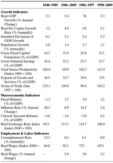
A.2 Macroeconomy of Chile
period the Terms of Trade was 143.2 with inflation rate of 3.4%. In the case of Chile an increase in the price of copper resulted in a reduction in domestic CPI inflation.
Chile adopted a policy of non-intervention in the exchange rates and thus has experienced higher variation in the nominal exchange rates in the 2000-2009 period. This increased volatility in exchange rates , not focusing on unemployment are some of the drawbacks of the Chilean approach to monetary policy with the sole goal of inflation targeting.
A.3 Inequality and Poverty
The Gini coefficient for Chile has been above 50 and constant through the last 20 years. Transition back to democracy, increases in GDP and per capita GDP did not affect the Gini coefficient and the underlying inequality in Chile. The constitution crafted under Pinochet and general low levels of empowerment reduce the amount of influence ordinary people have on public policy. This results in a lack of social services like public pensions, healthcare and good schooling.
Table 5.1 from Solimano (2012) shows the reduction in poverty and acute poverty in Chile. The recent economic prosperity and social programs targeted at the poor were successful in lowering the overall and the acute rates of poverty. These numbers are uplifting, however the methodology for calculating the official poverty rate was questioned by Larrain (2008). Additionally getting out of poverty is not permanent for all households in Chile. Lopez (2008) showed that a large part of the population is only slightly above the poverty line and any large exogenous shock can drive those households back into poverty. Chile is known for earthquakes that can wreak large scale damage even in the most adapted cities. The lack of a robust social net will mean that a large share of the population could fall into poverty in the case of a large earthquake.
reduction in institutional quality stemming from the Pinochet coup and repression should have resulted in a basketcase country. In the case of Chile both of those thing did not stop the country from growing and eventually joining OECD. It is possible that elite capture of resources and the deterioration in institutional quality happens over many decades and the past 20 years of democracy in Chile is not a long enough time horizon to see any significant effects. The problem of inequality is compounded by a very regressive tax system that heavily favors the rich over the poor and middle income citizens. The following Table 4 from Lopez(2007) provides an overview of the skewed tax system that provides 81% of tax loopholes to the top 5% of the income distribution.
Lagos and her successor Bachelet set out to change the goal of economic development in Chile by focusing on increasing social protection. The first aspect was reform of the anti poverty program Chile Solidario. This program provided cash assistance to some 300,000 families and also worked with those families to meet certain conditions over a two year period.
The education law implemented by the Pinochet regime was called Ley Organica Constitucional de Educacion (LOCE). The aim of that law was to privatize the educational system in Chile as much as possible. This resulted in a two tiered system with underfunded public schools for the poor and middle income people and a private school system for the wealthy. This resulted in university students being responsible for upto 80% of their tuition and fees. Student unions like Federacion de Estudiantes de Chile and Federacion de Estudiantes de la Pontificia Universidad Catolica de Chile protested this segregated system of education. Such a tiered system helps maintain the high inequality in Chile by denying poor and middle income students the opportunity for upward mobility through educational achievement. Efforts to reform this system were met with pushback from neoliberal forces in Chile, as the voucher system used in LOCE was the brain child of Milton Friedman. This voucher system split the educational system into three parts. Public schools, voucher subsidized schools and fully private schools.
Following massive student strikes in 2006 and 2011 president Bachelet introduced new laws governing education in Chile. Her reforms did not address the core stratification of the education system, but merely provided larger educational subsidies for low income and middle income households. The new subsidy covers preschool and primary school fees.
The Pinochet regime introduced privatization into the healthcare sector by dividing it into public and private parts. The public part, FONASA, insured access to healthcare for all. The poor people do not pay for their treatment in FONASA facilities. FONASA system is characterized by long waiting lines and under funded facilities. The private part is called ISAPRES and the fees for treatment are calculated based on the recipient's income. Healthcare sector underwent reform under the socialist governments of Lagos and Bachelet. The goal of this reform , titled AUGE, was to increase preventative treatment and increase access to treatment for lower and middle income Chileans. The military in Chile has its own health care service.
favored people in high paying white collar jobs over the majority of Chileans employed in small and medium businesses. The individual has to make at least 20 years of contributions to receive a minimum pension under this system. The privatized retirement system did contribute to the development of financial markets in Chile. Bachelet introduced reform that gave persons age 65 and over supplementary pension if they met certain criteria. This was done to help the poor people that do not receive a pension. Once again the military is exempt from the private pension system.
Since the restoration of Democracy , the military has enjoyed a privileged status in Chile. The command in chief of the Chilean army is not accountable to the civilian oversight. The military used to receive a set 10% of the revenues from the state owned copper company, CODELCO. This arrangement ended in 2009. Now the military is budgeted a nominal sum. This was done at the request of the military, because it wanted a stable source of revenue for its funding.
The Chilean experience of political instability is common in South America. Argentina has experienced repeated cycles of political turmoil from 1960 all the way up to 1990. Ecuador has experienced instability from 1960 to 1980. The Dominican Republic has experienced instability in the 1960s.
Chile ranks high in common measurements of good governance as defined by the World Bank. On the measurements of Voice and Accountability, Political Stability, Government Effectiveness, Regulatory Quality, Rule of Law and Control of Corruption Chile ranks much higher than its South American neighbors. For this reason Foreign Direct Investment has been an important part of copper mining sector's development in Chile. More recently FDI has flown into a variety of South American countries. Most of that investment has been into petroleum, natural gas and mineral production. In Chile Chinese FDI has been directed solely at the copper mining center.(Barton, 2009) Neoliberal reforms guaranteed private property rights and made Chile a relatively safer place for FDI than Bolivia, Ecuador and Venezuela. (Hogenboom, 2010; Kirby, 2010)
Chile has very low rate of investment into Research and Development. On average Chile spends about 0.5% of its GDP on R&D while other countries like Korea spend 2.6%, and Ireland spends 2.6%. The private sector in Chile does not contribute enough to Research and Development compared to other countries. In Sweden the private sector contributed 70% of all R&D, while in Chile the figure is only 26%. (Gregorio, 2005)
A.4 Copper Exports and Inflation in Chile
The main findings of my paper are confirmed in the case of Chile. An increase in the price of copper leads to a decrease in inflation. The following figure from Desormeaux(2009) shows that positive terms of trade shocks in Chile are negatively correlated with the inflation rate.
Desormeaux(2009) models both pro-cyclical and counter-cyclical fiscal policy. The following findings from Desormeaux(2009) suggest that Chile is engaged in counter-cyclical fiscal policy.
A.4 Conclusion