The University of San Francisco
USF Scholarship: a digital repository @ Gleeson Library |
Geschke Center
Master's Theses Theses, Dissertations, Capstones and Projects
Fall 12-16-2016
Phylogenetics, biogeography, and climate niche
variation of South Pacific and Hawaiian Psychotria
Elaine ZhangFollow this and additional works at:https://repository.usfca.edu/thes Part of theEvolution Commons
This Thesis is brought to you for free and open access by the Theses, Dissertations, Capstones and Projects at USF Scholarship: a digital repository @ Recommended Citation
Zhang, Elaine, "Phylogenetics, biogeography, and climate niche variation of South Pacific and Hawaiian Psychotria" (2016).Master's Theses. 222.
Phylogenetics, biogeography, and climate niche variation of South Pacific and
Hawaiian
Psychotria
by Elaine Zhang
Thesis
Submitted in Partial Satisfaction of the Requirements For the Degree of
Masters of Science In Biology
In the
College of Arts & Sciences University of San Francisco
San Francisco, California 2017
Committee in Charge
ABSTRACT
Why do some species have broad geographic distributions, while other species are confined to a narrow distribution? Species age, ecological niche, or dispersal traits may help explain why some insular species are abundant and found on many islands, while others are rare and restricted to one island. In this study, I inferred a robust, time-calibrated phylogeny of the Hawaiian Psychotria, using two nuclear and eight chloroplast loci, sampling 67 individuals. I coupled my phylogenetic hypothesis with climatic data, ecological niche modeling, and morphological dispersal characteristics to explain the variation in number of islands occupied by each species. My inferred phylogeny showed stronger support for many relationships among the Hawaiian species. Restricted lineages on the older islands were found to be basal, while younger, derived species were more widespread. The species that have managed to disperse to and colonize
multiple islands are the younger species. The biogeographical South Pacific Psychotria suggests
strong biogeographic structure, with early divergences of major clades and very few species subsequently dispersing and colonizing other geographic regions. Results of niche breadth and climatic niche models of the Hawaiian species indicate a general pattern of older species having narrower climatic niche breadths, which may explain their smaller geographic ranges. In contrast, the younger species have wider climatic niche breadths, which may explain why they occupy larger geographic ranges across multiple islands. However, multiple regression analysis indicate greater plant height (associated with dispersal abilities) has the strongest weight in
ACKNOWLEDGMENTS
I would like to first thank my thesis advisor, Dr. John R. Paul of the College of Arts & Sciences at University of San Francisco (USF). I cannot express enough gratitude and appreciation for all the support and opportunities he has given me. His guidance and exceptional knowledge helped steer me in the right direction at times when there were questions about the research or writing. His encouragement and belief has allowed me to push my boundaries and become a more confident scientist and researcher. He will always be a great advisor, mentor, professor, colleague, and friend. I give my sincerest thanks for everything and for the continuous support.
I would also like to thank my thesis committee: Dr. John R. Paul, Dr. Sikes, and Dr. Nunes of the College of Arts & Sciences at USF. I am grateful for all the guidance and valuable inputs they provided for thesis to be completed successfully.
This thesis project would not have been completed had it not been for the National Tropical Botanical Garden (NTBG) in Kauai for allowing herbarium sampling of Psychotria species. I would like to give thanks to our collaborators, Dr. David Lorence and Dr. Kenneth Wood at NTBG, and Dr. Kenta Watanabe of Okinawa National College of Technology in Okinawa, for especially curating the samples, and for being great mentors in the field during our research expedition in Kauai.
I would also like to thank the University of San Francisco Faculty Development Fund (FDF) for allowing my research to take place in the Biology Department of University of San Francisco. And thanks to the faculty and staff in the Biology Department, members of the John Paul Lab, and Dr. April Randle, with whom I got the chance to work with and got to know throughout my time in the program.
TABLE OF CONTENTS
TOPIC PAGE
ABSTRACT ………...….… i
ACKNOWLEDGMENTS ……….………..………... ii
LIST OF TABLES ……….………..………... iii
LIST OF FIGURES ……….……….………... iv
INTRODUCTION ……….….…1
METHODS ………....………...…...… 11
Molecular Methods ………....……….….… 15
Phylogenetic Methods ………....………..….... 24
Ecological Niche Modeling ……….…...…….……….... 28
Dispersal Ability ……….. 30
Statistical Tests ………..………..… 30
RESULTS ………...…………..…..,,,.…….… 32
Phylogenetic Analyses ………...……...….…….… 32
Divergence Time Estimates ………...………....…………..… 33
Ecological Niche Models ....………....……….……....… 39
Statistical Analyses ………..………..………..… 40
DISCUSSION ……….………..……..……….…… 42
TABLES ………....……….…. 52
FIGURES ………....……….…....…… 76
APPENDICES ………...……...……. 110
LIST OF TABLES
TABLE PAGE
Table 1. Characteristics and locations of Hawaiian Psychotria species. …………..………..… 52
Table 2. Taxon samples of Hawaiian and South Pacific Psychotria species used in study. …... 53
Table 3. Hawaiian and South Pacific Psychotria species from GenBank used for study. ...…... 57
Table 4. Psychotria species outgroups from GenBank used for study. ………... 62
Table 5. Nuclear ribosomal and chloroplast markers used in study. ………….………....…..… 63
Table 6. Characteristics of nuclear and chloroplast loci genomes used for inferring phylogenies. ………..… 64
Table 7. Concatenated alignments used in study to infer phylogenies of Hawaiian and South Pacific Psychotria. ……….... 64
Table 8. Occurrence data of Hawaiian Psychotria species. ……….... 65
Table 9. Global Climatic Data obtained from WorldClim. ……….…… 70
Table 10. Divergence times of the Hawaiian Psychotria. ………....……... 71
Table 11a. Model statistics from BioGeoBEARS analysis using BEAST Chronogram – Hawaiian and South Pacific Psychotria, 6 Loci. ……….… 71
Table 11b. Model statistics from BioGeoBEARS analysis using BEAST Chronogram – Hawaiian Psychotria, 6 Loci. ………..… 71
Table 12. Niche breadths of Hawaiian Psychotria. ……….… 72
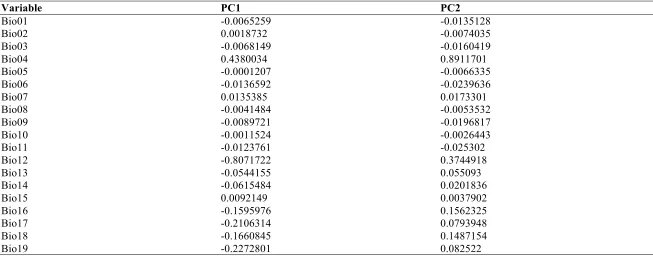
Table 13a. Variable loadings from a principal component analyses of 19 bioclimatic variables for the Hawaiian Psychotria. ………..………..…... 73
Table 13b. Variable loadings from a principal component analyses of 19 bioclimatic variables for South Pacific and Hawaiian Psychotria, using species means. ……..… 74
LIST OF FIGURES
FIGURE PAGE
Figure 1. Distribution of Hawaiian Psychotria species on the Hawaiian Islands. ..…………... 76
Figure 2a-c. Bayesian phylogeny of Hawaiian and South Pacific Psychotria species inferred using 8 loci markers (ITS, ETS, psbA, psbE, rbcL, rps16, tnK, and trnT). ... 77
Figure 3a-c.Bayesian phylogeny of Hawaiian and South Pacific Psychotria species inferred using 6 loci markers (ITS, ETS, matK, psbA, rbcL, and rps16). ………...… 80
Figure 4a-c.Bayesian phylogeny of Hawaiian and South Pacific Psychotria species inferred using 3 loci markers (ITS, ETS, and rps16). ………... 83
Figure 5a-c.Bayesian phylogeny of Hawaiian and South Pacific Psychotria species inferred using 6 loci markers (ITS, ETS, matK, psbA, rbcL, and rps16), with
ages on clade. ……….…... 86
Figure 6a-c. Bayesian phylogeny of Hawaiian and South Pacific Psychotria species inferred using 6 chloroplast loci markers (psbA, psbE, rbcL, ps16, trnK, and trnT). …….….. 89
Figure 7a. Biogeographic history of Hawaiian and South Pacific Psychotria inferred using 6 loci markers (ITS, ETS, matK, psbA, rbcL, rps16) under the DEC+J model
(on the BEAST chronogram) in BioGeoBEARS analysis. ………..… 92
Figure 7b. Biogeographic history of Hawaiian Psychotria inferred using 6 loci markers (ITS, ETS, matK, psbA, rbcL, rps16) under the DEC+J model (on the BEAST
chronogram) in BioGeoBEARS analysis. ………..………... 93
Figure 8.Haplotype network of Hawaiian Psychotria inferred using 6 chloroplast loci
markers (psbA, psbE, rbcL, rps16, tnK, and trnT). ………..… 94
Figure 9a-m. Ecological Niche Models of Hawaiian Psychotria. ………...…. 95
Figure 10a. Plot of the first two PCs of 19 bioclimatic variables across the Hawaiian
Psychotria species. ………... 108
Figure 10b. Plot of the first two PCs of 19 bioclimatic variables across 36 South Pacific
INTRODUCTION
Understanding the factors that regulate the abundance and distribution of organisms is a central
goal of ecological research. Species vary dramatically in their absolute abundances and
geographic ranges sizes (Gaston 2003). Much of this variation is expected, given the unique
ecological niches, specialized habitats, and ways of making a living that organisms possess.
However, even closely-related species that are remarkably similar in their attributes can vary
greatly in their abundance and distribution (Gaston 2003; Paul et al. 2009).
What factors are most important in driving the variation in abundance and distribution of
closely-related species? This is a complicated and multifaceted question that likely has many
answers depending on the lineages that are studied. Explaining variation in abundance has
traditionally been the purview of ecological studies focusing on proximate causes (Ricklefs
2008). In local communities, competition, predation, herbivory, and mutualistic interactions have
all been shown to be important drivers of variation in abundance (Ricklefs 1987). When taking a
more regional perspective, variation in the distribution of organisms can be viewed by
contrasting their geographic range sizes.
Only more recently have studies started to explicitly incorporate an evolutionary perspective
(Paul et al. 2009) on variation in abundance and distribution. Evolutionary history has been
proposed to be important in particular to explain variation in distributions as quantified through
proposed to explain variation in range size of closely-related species. First, species age was
proposed to be important to geographic range size in the 1920s by John Willis (Willis 1922),
whose ‘age-and-area hypothesis’ predicted many species with small geographic ranges are
simply evolutionarily young species. Recently, some empirical evidence has been found for this
pattern (Paul et al. 2009), but other studies have found no relationship between species age and
range size (Jones et al. 2005). Further, Pigot et al. (2012) used simulations to argue that
directional range size evolution patterns are mainly an artifact of the processes of speciation and
extinction. Conversely, others have proposed that many species with restricted geographic ranges
are ‘relict species’ – species that once had larger ranges but have failed to adapt to changing
climatic conditions (Murray & Hose 2005). The California redwoods and sequoias have been
proposed as such lineages (Florin 1963), as their clade once had a much broader global
distribution. However, Ricklefs (2012) argued that overall species age shows little consistent
relationship with range size and hence is a weak predictor.
If species age alone can’t explain range size variation, it doesn’t lessen the importance of an
evolutionary perspective, as species inherit their characteristics from their ancestors, and lineages
may vary in how quickly characteristics evolve. Of particular interest to geographic ranges is the
ecological niche, which can be defined as the set of ecological conditions in which a given
species can maintain stable or positive population growth (Angert 2009). Variation in ecological
niches, and by extension, the ecological tolerances of species, should be critical in determining
spatial manifestations of the ecological niche (Pulliam 2000), and as such, provide a means to
quantify and compare the ecological niches of species.
The relationship between ecological niches and geographic ranges has been examined through
lens of niche breadth, the range of environmental conditions a species can tolerate, and niche
lability, the ability of a lineage to transform its ecological niche characteristics over time. Species
with broader ecological niches may be expected to have larger geographic ranges (Slayter et al.
2013; Sheth & Angert 2014), simply because these species can occupy a greater proportion of
ecological niche space distributed in the environment. As a corollary, species with narrow niche
breadths that can only tolerate a limited set of ecological conditions are expected to have smaller
geographic ranges. Of course, these predicted patterns can be easily thrown into array, if for
example, a particular habitat that a species with a narrow niche breadth specializes on is
abundant and widespread across the landscape. Empirical evidence for the relationship between
niche breadth and range size is somewhat sparse, but recent research has been support (Sheth &
Angert 2014) and some argue for the generality of this relationship (Slayter et al. 2013).
How quickly a lineage or species’ ecological niche evolves may also have an impact on
geographic distributions. Similar to a species with a broad ecological niche, a species that can
evolve its ecological niche characteristics quickly may also rapidly transform its geographic
range size. Such niche labile lineages can be exemplified through adaptive radiations – rapid
diversification and niche expansion via adaptive evolution (Givnish et al. 2009). The Hawaiian
Phylogenetic analysis of the Hawaiian silverswords shows they share a common ancestor with a
clade of California tarweeds, and suggest a single dispersal event less than 6 mya founded the
original Hawaiian ancestral population (Baldwin et al. 1991). From there, over 50 distinct
species have evolved over the course of only 5 my. Most remarkable though is the ecological and
morphological variability this clade expresses, with some Hawaiian species being small seaside
herbs, similar to the California tarweeds, and some being succulents, woody climbers, shrubs,
and even trees. Furthermore, this clade has a very broad climatic niche with the sum of the
species distributed across all islands, from sea level to over 3000 m elevation on Mauna Kea,
Hawaii. In contrast, species that evolve their ecological niche characteristics slowly may fail to
expand their geographic ranges over evolutionary time. Such species exemplify niche
conservatism, the tendency of species to maintain the ecological niches of their ancestors (Wiens
et al. 2010). Niche conservative species may also have increased difficulty maintaining species
cohesion because of barriers to gene flow imposed by tracts of unsuitable habitat, leading
ultimately to lineage splits in the absence of substantial ecological niche evolution (Wiens et al.
2010).
Recently, ecological niche modeling (ENM) methods have been developed to estimate a species’
climatic niche characteristics using geographic distribution data (Phillips et al. 2004; Phillips et
al. 2006). Specifically, this set of methods uses the geographic coordinates from collection
records of a given species to extract a set of climatic variables (e.g., mean annual precipitation,
mean annual temperature, etc.) from a global database (e.g., WorldClim, Hijmans et al. 2005) for
collection records, the predicted ecological niche conditions in which a species can occur is
estimated, and a predicted geographic range can be extrapolated. The practicality of these
methods is enhanced by the subset of methods that only requires presence points (e.g., collection
records from a museum or herbarium) to estimate the niche, but requires no absence points
(which are typically unknown). The utility of these methods has led to an explosion of studies
incorporating ENMs to answer a wide range of questions, from conservation purposes
(Raxworthy et al. 2003) to the evolution of climatic niches (Kozak and Wiens 2010; Title &
Burns 2015), and the explanations of patterns of diversification and species richness (Kozak &
Wiens 2010).
Dispersal by definition is required to expand a species’ geographic range, so naturally variation
in dispersal ability has been proposed to be an important factor (Brown et al. 1996; Iversen et al.
2013). Dispersal is the ecological process where individuals move away from their source
population to novel habitats. In some cases, dispersal ability appears to be more important than
ecological tolerances to predict geographic range size (Arribas et al. 2012). Yet despite the
intuitive importance of dispersal characteristics, their ability to explain variation in geographic
range size has been limited (Lester et al. 2007; Gove et al. 2009).
Islands provide a unique setting to examine distributions and have played an important role in
ecological and evolutionary theory (Whittaker et al. 2008; Gillespie & Baldwin, 2010). Island
biogeography is a theory that explains the factors and biological processes that affect species
and in rates of colonization and extinction (MacArthur & Wilson 1967). Oceanic islands provide
a unique and effective model for testing geographical and ecological properties influencing
endemic diversity (MacArthur & Wilson 1967). More recently, the ‘General Dynamic Model of
Oceanic Island Biogeography’ (Whittaker et al. 2008), states diversification is greatest on larger
islands that are remote, allowing for rapid diversification amongst the few lineages that manage
to colonize remote islands (MacArthur & Wilson 1967). In addition, islands are often comprised
of novel habitats that may promote rapid evolution of new adaptations (Bennett et al. 2013),
ultimately leading to adaptive radiation. Island radiations are driven by island colonization via a
founder event and subsequent genetic divergence from source populations via natural selection
and genetic drift (Dixon et al. 2011). Evolutionary processes that underlie island adaptive
radiations, such as how species diversify in these novel ecological niches given new resources
within confined geographical regions (Schluter 2000), still remain unclear (Kapralov et al. 2013).
However, key adaptive radiations on islands have been viewed to follow similar processes as on
continents, thus examining islands can provide a general understanding of adaptation and the
drivers of species diversity (Emerson 2002).
Colonization of islands is driven by a species’ dispersal abilities (Fritz et al. 2012). Dispersal is
an important factor regulating whether colonization events are successful and whether species
subsequently spread across island archipelagos, ultimately influencing patterns of species
distribution and abundance. If dispersal abilities are low, colonization events may lead to species
divergence and possibly speciation. However, if dispersal abilities are high, gene flow can occur
ecological niche conditions due to limited range size (Kapralov et al. 2013). Therefore, limited
ecological space may restrict diversity due to decrease in genetic variability within a small
population size (Dixon et al. 2011). However, steep ecological gradients can promote diversity
within a small amount of ecological space, especially among species with high dispersal abilities
(Frankham 1997). Islands also exhibit taxon cycles, defined as the cyclic evolution of species (Wilson 1961) where species’ ranges undergo sequential phases of expansion and contraction
resulting in shifts in relative distribution and abundances of species across islands (Ricklefs et al.
2002). Taxon cycles can provide understanding of distribution and extinction patterns across
island chains by examining interactions between colonizing and resident species. Such
interactions can give rise to gaps in island occupancy if either the novel or native species faces
extinction due to genetic divergence between island populations after colonization from one
island to another, thus leading to range contraction (Ricklefs et al. 2002). The causes of taxon
cycles are unknown, but have thought to be driven by coevolution among novel and native
species (Ricklefs et al. 2002).
In this study, I use the Hawaiian Psychotriadiversification as a model system to understand the drivers of variation in abundance and distribution. Psychotria (Rubiaceae; the coffee family) is one of the most species rich genera of plants in the world (~1600 species; Paul et al. 2009) and
pantropical in distribution with diversifications across various continents and islands of the South
Pacific and the Caribbean (Nepokroeff et al. 2003). South Pacific islands have many endemic
and very few widespread species, whereas in the Caribbean there are fewer endemics and more
pantropic distribution suggests considerable dispersal abilities among species of Psychotria, which typically have red, blue, orange or purple fruits that are dispersed by birds. However some
species within Psychotria have remained confined to single oceanic island (or in a continental setting, mountaintop or unique habitat island) and do not disperse across islands. Why is this the
case? Species of Psychotria also vary tremendously in geographic range size, both generally (Paul et al. 2009) and specifically in Hawaii. Psychotria grandifloraand Psychotria hobdyi, for example, both have very small range sizes and are only found on the northwest corner of Kauai,
the oldest island of the Hawaiian Islands. In contrast, Psychotria marinianaexhibits a relatively larger geographic range and is found distributed across multiple Hawaiian islands: Kauai, Oahu,
Molokai, Lanai, and Maui (Nepokroeff et al. 2003). Why do these closely-related species vary so
greatly in their distributions? Previous work has shown that some Psychotriaspecies transform their ranges slowly (rare species = young species; Paul et al. 2009). This suggests species of
Psychotria are good at dispersing over long distances over long time periods, but are slow to
expand their range size in absolute time. Other recent work reveals Psychotriaspecies exhibit phylogenetic niche conservatism in climatic characteristics, with the inferred climatic niches of
ancestral species being a strong predictor of microhabitat associations in Neotropical species,
even after millions of years of divergence and dispersal (Sedio et al. 2013). Do Hawaiian
Psychotria display similar evidence of conservatism in climatic niche traits? Do species that
inhabit many islands occupy similar or different climatic niche space on different islands? And
are species that have colonized multiple islands also those with the greatest climatic niche
Hawaiian Psychotria are a relatively small radiation with 11 recognized species and numerous named subspecies and/or varieties (Nepokroeff et al. 2003) that provide a textbook example of
older-to-younger island colonization (see Fig. 6.11 in Futuyma 2013). In previous phylogenetic
work, Nepokroeff et al. (2003) used two nuclear ribosomal DNA markers (ITS and ETS) to build
the first phylogeny of Hawaiian Psychotria species relationships. This pioneering work laid the groundwork for future work in Hawaiian Psychotria. However, one obvious limitation of this study was the use of only two loci, both of which are ribosomal nuclear markers. As a result,
they found low support for the inferred relationships between some of the younger Hawaiian
species (Nepokroeff et al. 2003). In addition, this study did not incorporate any chloroplast
markers, yet some chloroplast markers can be useful for species-level discrimination, particularly
when paired with nuclear markers such as ITS (China Plant BOL Group et al. 2011). Nepokroeff
et al. (2003) also sequenced relatively few samples for a given species, and their results point to
some species with multiple accessions as non-monophyletic, especially when the same putative
species was sampled on different islands. This calls for more collections of individuals per
species as well as using additional nuclear and chloroplast markers to develop a robust
phylogeny of Hawaiian Psychotria in order to resolve these relationships. The initial Nepokroeff et al. (2003) phylogeny was used as a test case for a new method for inferring geographic range
evolution (Ree & Smith 2008), and then again to test yet another new method (Matzke 2014), but
a better phylogeny would help to more accurately infer geographic range evolution. Hawaiian
Psychotria exhibits variation in distribution within and across the Hawaiian islands, which prompts the following general questions. Why do some species occupy one or two islands, while
others are more common? Can species’ climate niche or dispersal characteristics help explain
these patterns?
For this thesis, I had six specific objectives:
1) Develop a robust molecular phylogenetic hypothesis for the evolutionary relationships of
Hawaiian Psychotria species using multiple nuclear and chloroplast DNA markers and multiple, widely-sampled individuals per species.
2) Infer the climatic niches of the Hawaiian Psychotria species and calculate their climatic niche breadth using georeferenced collection records.
3) Test for the relative importance of three factors, species age, climatic niche breadth, and
dispersal characteristics (seed size, body size), in explaining the variation in geographic
distribution among species.
4) Build a more extensive molecular phylogenetic analysis of South Pacific Psychotria
species by sequencing new species and combining my new data with previously
published sequences.
5) Infer the ages and biogeographic history of the Hawaiian and South Pacific Psychotria
species.
METHODS
Study Taxa and Ecological Context
The 11 Hawaiian Psychotria species are distributed across the six largest Hawaiian islands of
Kauai, Oahu, Molokai, Lanai, Maui, and Hawaii (Fosberg 1962, 1964; Sohmer 1977; Table 1).
The Hawaiian species are mostly comprised of small trees and shrubs and are endemic to the
Hawaiian Islands (Sohmer 1977). The number of independent introductions of Hawaiian
Psychotria has been debated, with hypotheses stating either a single independent introduction
(Fosberg 1962) or multiple (2 or 3) independent introductions (Sohmer 1978) resulting in the
Hawaiian Psychotria. Taxonomically the genus,Straussia, as described by Asa Gray (1858) has long caused difficulties for accurate classification of Hawaiian plant species within Psychotria, due to high taxon complexity likely resulting from rapid diversification and hybridization among
species of Straussia across the islands (Nepokroeff et al. 2003). In the early 1960s, F.R. Fosberg (1964) formally classified Straussia as a section withinPsychotria, and described an additional section calledPelagomapouria (Sohmer 1977). The section Straussiais comprised of P. fauriei, P. greenwelliae (formerly namedP. psychotrioides), P. hathewayi, P. hawaiiensis, P. kaduana, P. mariniana, P. mauiensis, and P. wawrae. The section Pelagomapouria is comprised of P. grandiflora, P. hexandra, and P hobdyi . The classification of these divergent sections within Hawaiian Psychotria led S.H. Sohmer (1977) to hypothesize multiple independent colonization events rather than a single introduction onto the Hawaiian Islands. However, this theory
Pelagomapouria species, which are found on older islands and tend to be the most distinct from
one another (Sohmer 1978). Unlike the Pelagomapouria species, members of the Struassia
section are more widely distributed across multiple islands. As they undergo adaptive radiation
and/or hybridization after a dispersal event, they may tend to lose integral characteristics that
allow for theses species to be easily distinguished from one another (Sohmer 1978). Recently
Nepokroeff et al. (2003) inferred the first phylogeny of Hawaiian Psychotria, which revealed a significant finding. The Hawaiian species all formed a clade, indicating a single dispersal event.
Furthermore, Nepokroeff et al. (2003) did not infer a time-calibrated tree, but they found a
pattern of short branch lengths as is often found in phylogenies of other Hawaiian taxa (e.g., the
Hawaiian silverswords; Baldwin 1991) that suggest a rapid radiation following a single
introduction.
The Hawaiian Islands are the most isolated archipelago in the world (Fleischer et al. 1998) and
home to over 1000 endemic plant species. The eight main islands (Niihau, Kauai, Oahu,
Molokai, Lanai, Maui, Kahoolawe, and Hawaii) are composed in a linear array; from northwest
to southeast arrangement. The Hawaiian Islands were established as the Pacific tectonic plate
shifted and moved over volcanic regions (known as hot spots) forming a trail of active
volcanoes. As islands shift away from the hot spot, they undergo subsidence and erosion creating
atolls and seamounts (Fleischer et al. 1998). Potassium-argon (K-Ar) dating on lava surfaces of
the Hawaiian Islands initially reported by I. McDougall (1964) suggests a methodology for
island age estimation (Funkhouser et al. 1968). The oldest island of Kauai is dated at 5.1 million
1.32-0.75 Ma, and the youngest island of Hawaii is estimated to be at 0.43 Ma (Clague &
Dalrymple 1987). Further K-Ar dating from Carson & Clague (1995) suggested the Maui, Lanai,
Molokai, and Kahoolawe islands were connected around 0.3-0.4 Ma, an island known as Maui
Nui. After formation of West Molokai, the island was connected to Oahu for a duration of 0.3
million years (Carson & Clague 1995). The Hawaiian islands are an exemplary model for island
biogeography studies because age determination of individual islands via K-Ar dating can allow
island age to be associated to biological events such as speciation (Dixon et al. 2011).
In the larger context of the South Pacific, island chains across the Pacific were formed from hot
spots caused by the subduction of the Pacific Plate and now extinct Izanagi and Kula plates
(Neall & Trewick 2008) , generating numerous linear arrays of magma-filled volcanic arcs and subsequent submarine seamounts. Especially during Quaternary time, there were additional
processes that influenced the formation of these islands such as fluctuating sea levels during
periods of glaciations and interglaciation, which created the effect of linking islands and greatly
influenced biodiversity across islands (Neall & Trewick 2008) . Across Oceania, there are five subregions of islands. Continental Asia includes islands such as Japan, Philippines, Palau, Bonin
Islands, and Taiwan. Japan consists mainly of four big islands, referred to as the ‘Home Islands’:
Hokkaido, Honshu, Shikoku, and Kyushu. In addition there are over 6000 smaller islands within
the archipelago of Japan which happens to be the largest archipelago in the Pacific, formed by
the subduction of the Pacific plate beneath the Eurasian plate (Neall & Trewick 2008) . Japan is mountainous and still holds volcanic activity. The Izu-Bonin-Islands extend off the coast of
in between 50 and 40 Ma (Neall & Trewick 2008) . Palau consists of 12 inhabited and over 700 small islands encased with rich and diverse landforms and climate. As a result, there is a large
number of endemic species and the flora is richest in Palau compared to other regions of
Micronesia (Canfield 1981). The subregion Melanesia, consists of the Solomon Islands, Papua
New Guinea, Fiji, New Caledonia, and Vanuatu. The Solomon archipelago is comprised of seven
major Solomon islands spanning the western Pacific Ocean along with islands of Papua New
Guinea. Most regions of the Solomon Islands are of dense tropical rainforest with consistent
annual temperature (28-30°C; Neall & Trewick 2008). Fiji consists of 332 islands, with the two largest being Vanua Levu and Viti Levu. Fiji has a very mountainous landscape where it was
once covered in dense tropical rainforest (Neall & Trewick 2008). New Caledonia is comprised
of the Grande Terre Island, Isle of Pines, and the Loyalty Islands. The mountains on Grande
Terre form a divide on the island, humid east coast and dry west coast (Neall & Trewick 2008).
Low levels of nitrogen, potassium, calcium, phosphorus in the soil on New Caledonia drive flora
richness (Jaffre et al. 1987). The Polynesia subregion includes New Zealand, Samoa, Society
Islands, and Austral Islands. Around 90 Ma a land mass known as Zealandia, began to separate
from Gondwana and underwent sea-floor spreading and subsiding, eventually forming the region
of New Zealand (Mortimer 2004). New Zealand today consists mainly of two large islands,
North and South Island, and two small islands, Chatham and Stewart. The Society Islands are
comprised of five groups, two of which are the main island of Tahiti and French Polynesia. This
tropical archipelago was thought to have formed from a hotspot near Mehetia island, one of the
Society Islands, east of Tahiti (Devey et al. 1990). Its mean annual rainfall range is 1700 mm
2008). Continental Australia, the last subregion, consists of Australia, Tasmania, and a large
number of smaller islands.
Remarkably, Psychotria species have managed to colonize all the subregions mentioned above, despite the large area encompassed by Oceania and the huge distances of unsuitable habitat
(ocean) separating successful colonizations. There has been a massive diversification (> 100) of
Psychotria species in New Caledonia ( Barrabé, et al. 2014), and Fiji, Samoa, and the Mariana Islands all have sizable but poorly described species pools. In addition, the Philippines has over
100 described species (Sohmer & Davis 2007), including many endemic species, although due to
catastrophic deforestation over that past few decades, many of these species are likely extinct.
Finally, Papua New Guinea likely also harbors well over 100 species, many of which remain
undescribed (S. Sohmer, personal communication with J. Paul).
MOLECULAR METHODS
Sampling of Taxa and DNA Extraction
For this study I obtained vouchered leaf tissue samples and some of the species included are
represented by multiple individuals (refer to Table 2). I obtained silica-dried samples from six
Hawaiian Psychotriaspecies (two of which are P. grandifloraandP. hobdyi, federally listed rare and endangered species) and eight South Pacific Psychotriaspecies from the collections of the National Tropical Botanical Garden (NTBG) in Kauai, Hawaii with the help of our collaborators,
Dr. David Lorence and Dr. Kenneth Wood at NTBG. The few previously sequenced South
Nepokroeff et al. (2003). I also obtained samples from 15 New Caledonian Psychotria species from the Missouri Botanical Garden in St. Louis, Missouri. In addition, our collaborator, Dr.
Kenta Watanabe of the Okinawa National College of Technology in Japan, who is studying the
breeding systems of Hawaiian Psychotria, shared silica-dried leaf tissue samples of his collections with us, which included samples from 10 Hawaiian and six Japanese Psychotria
species, most represented by multiple individuals. DNA from leaf samples was extracted using a
modified version of the Alexander et al. (2007) protocol for plant DNA extraction. All extracted DNA products were run on 1.5% agarose gel using GelRed and observed for band brightness
under ultraviolet light to determine extraction quality.
DNA Marker Selection
The Hawaiian and South Pacific Psychotria samples I acquired were used to amplify and sequence a set of DNA markers (nuclear ribosomal and chloroplast) for phylogenetic inference.
Nuclear markers included in this study were the internal- and external-transcribed spacer (ITS
and ETS, respectively) regions of the nuclear ribosomal DNA genome. The ITS/ETS markers are
generally easy to amplify via polymerase-chain reaction (PCR), widely used, and can be
phylogenetically informative (Álvarez & Wendel 2003), particularly when used together
(Logacheva et al 2010). However, these loci can be problematic in some taxa because they are
multicopy loci (Baldwin et al. 1998), meaning that it can be potentially difficult to distinguish
orthologs (homologous loci) from paralogs (gene duplications). In many taxa the multiple ITS
copies appear to undergo concerted evolution via homologous recombination (Naidoo et al.
than to members of their own gene family in other taxa. Hence, in taxa that have strong
concerted evolution, the multicopy nature of these ribosomal markers does not impede their
phylogenetic utility, and in fact ITS has been one of the most widely used and successfully
employed nuclear markers for species-level plant phylogenies (Pozcai & Hyvönen 2009).
Furthermore, since the nuclear genome is diploid (or of a greater ploidy), the effective population
size of the nuclear genome is twice that (or more) of the haploid chloroplast genome. This is
critical because it means that on average nuclear gene copies take twice as long to coalesce in the
past compared to plastids genes; hence nuclear genes in recently diverged species may retain
ancestral polymorphisms, leading to incomplete lineage sorting between loci, and the potential to
infer false evolutionary relationships (Pillon et al. 2013).
The plastid regions of the chloroplast DNA genome known as chloroplast markers have played a
central role in plant phylogenetics, especially for inferring generic and family-level relationships
(Palmer 1985; Kårehed et al. 2008). For inferring low-level phylogenetic relationships, some
chloroplast loci, particularly ‘class II introns’ (e.g., matK, rps16) have proven useful (Kelchner
2002). Chloroplast markers can often be amplified by near universal primers that are located in
highly conserved exons (Kelchner 2002), and in most angiosperm lineages chloroplasts are
maternally inherited via seeds, and reflect the history of seed dispersal and colonization within a
lineage (Patwardhan et al. 2014). In addition, the chloroplast genome has other traits that are
generally beneficial for phylogenetic inference - it is haploid and most loci are single copy
(Kelchner 2002). A haploid genome means that on average chloroplast gene coalesce two times
faster than nuclear genes, so chloroplast markers can show reciprocal monophyly between
plant chloroplast genome has a slower rate of evolution than the nuclear genome (Clegg et al.
1994), so chloroplast markers, when used individually or when only a few loci are combined,
may lack sufficient variability to be useful for species-level phylogenetics (Pillon et al. 2013).
However, recent research has identified additional chloroplast markers that appear to be highly
variable across species and potentially useful for infrageneric studies (e.g., Dong et al. 2012).
Combining nuclear ribosomal and chloroplast markers can be particularly beneficial for
successful plant species discrimination (China Plant BOL Group et al. 2011).
In general, the ribosomal nuclear and chloroplast markers described above often used for
barcoding are known to work well in Psychotria and other genera withinRubiaceae. Thus these markers were used in this study to infer phylogenetic relationships between the Hawaiian
Psychotria species (Table 5).
PCR Amplification - Nuclear Ribosomal Genome
Two nuclear ribosomal regions, the internal- and external-transcribed spacers (ITS and ETS),
were amplified with their respective forward and reverse primers. The PCR reactions were
carried out in reaction volumes of 25.63μL: 18μL pure H20, 2.5μL 10X Buffer, 2.5μL MgCl2, 0.5μL BSA, 0.5μL DMSO, 0.5μL dNTPs, 0.25μL forward and 0.25μL reverse primers, 0.125μL Taq, and 0.5μL DNA template. For the ITS region, the reactions were run using the
following thermocycler conditions: 2 min at 94 °C, 40 cycles of 30 sec at 94°C, 1 min at 48°C, and 1 min at 72°C, with an elongation period of 7 min at 72°C and final storage at 12°C (Sedio et
conditions: 3 min at 94 °C, 35 cycles of 30 sec at 94°C, 1 min at 50°C, and 1.5 min at 72°C, with an elongation period of 7 min at 72°C and final storage at 10°C (Barrabé et al. 2012).
PCR Amplification - Chloroplast Genome
The plastid regions were amplified with their respective forward and reverse chloroplast primers.
PCR reactions for the following primers (psbE-petL, trnK-rps16, and trnT-psbD) were carried
out in reaction volumes of 25.63μL: 18μL pure H 20, 2.5μL 10X Buffer, 2.5μL MgCl2, 0.5μL BSA, 0.5μL DMSO, 0.5μL dNTPs, 0.25μL forward and 0.25μL reverse primers, 0.125μL Taq,
and 0.5μL DNA template. The PCR reactions were run using the following thermocycling
conditions: 5 min at 94 °C, 30 cycles of 1 min at 94°C, 30 sec at 54°C, and 45 sec at 72°C, with an elongation period of 5 min at 72°C and final storage at 12°C (Dong et al. 2013). PCR reactions for primers (matK-kim, psbA, rbcL, and rps16) were performed using the mentioned
protocol in reaction volumes of 25.63μL. The samples were run using the following thermocycling conditions: 3 min at 94°C, 35 cycles of 1 min at 94°C, 1 min at 50°C, and 2 min
at 72°C, with an elongation period of 7 min at 72°C and final storage at 10°C (Barrabé et al.
2012).
DNA Clean-Up and Sequencing
All amplified PCR products were run on 1.5% agarose gel using GelRed and observed for band
brightness under ultraviolet light to determine the quality of amplification. Successful PCR
products were cleaned up using the following exonuclease I-shrimp alkaline phosphatase
Buffer, SAP, and EXO, and 7.5μL of PCR product. The cleaned-up PCR products were run on 1.5% agarose gel to check for the presence of successful bands. The purified PCR products were
sent to two sequencing facilities to obtain reads of forward and reverse DNA sequences: the
Cancer Research Center DNA Sequencing Facility in University of Chicago, Chicago, Illinois
and the Molecular Cloning Laboratories (MCLAB) in South San Francisco, California.
DNA ALIGNMENTS
DNA alignments of the sequences were performed using MUSCLE algorithm (Edgar 2004) in
the program Geneious v8.1.3 (Kearse et al. 2012). Alignment columns were manually edited to
ensure the polymorphic sites were indeed polymorphic, ambiguous sites were coded as N, and all
heterozygous sites from nuclear markers were assigned the proper ambiguity code (e.g., Y
represent C or T). Final consensus sequences of the alignments were generated from the edits
and used for phylogenetic inference (Table 6). I incorporated additional Hawaiian and South
Pacific Psychotria species sequences retrieved from GenBank (Table 4) into phylogenetic analyses.
A Core Phylogeny of Hawaiian and South Pacific Psychotria
The first objective was to build on the previous phylogenetic work of Hawaiian Psychotria, performed by Nepokroeff et al. (2003), by utilizing more nuclear markers and introducing
chloroplast markers for the first time. In addition, I incorporated more herbaria collections (i.e.
multiple accessions per species and multiple accessions per island and/or regions of islands). I
included both the two nuclear (ITS and ETS) and six chloroplast (psbA, psbE, rbcL, rps16, trnK,
and trnT) genes.
An Extended Phylogeny of Hawaiian and South Pacific Psychotria
The second objective was to expand on our robust phylogeny by incorporating additional Genbank sequences of Hawaiian and South Pacific Psychotria from previous studies in order to strengthen the inferred relationships among the Hawaiian species and infer which South Pacific
species is the closest relative to Hawaiian Psychotria. I inferred the phylogeny using Bayesian analyses with the 6-Loci alignment (Table 7), which included both the two nuclear (ITS and
ETS) and four chloroplast (matK, psbA, rbcL, and rps16) genes.
A Combined ITS, ETS, and rps16 Phylogeny of Hawaiian and South Pacific Psychotria
The third objective was to build a supermatrix phylogeny of Hawaiian and South Pacific
Psychotria by utilizing more taxa samples of Psychotria from Genbank in order to observe any evolutionary changes in the nuclear genome of Hawaiian and South Pacific Psychotriacombined with the rps16 chloroplast genome. I inferred the phylogeny using Bayesian analyses using the
3-Loci alignment (Table 7), which included both the two nuclear (ITS and ETS) genomes and
the rps16 chloroplast genome.
A Chloroplast Phylogeny of Hawaiian and South Pacific Psychotria
The fourth objective was to build a chloroplast phylogeny of Hawaiian and South Pacific
the chloroplast genome of Hawaiian and South Pacific Psychotria. I inferred the phylogeny using Bayesian analyses using the Chloroplast-Loci alignment (Table 7), which included 6 chloroplast
(psbA, psbE, rbcL, rps16, trnK, trnT) genomes.
I chose to utilize these four main alignments to infer phylogenetic relationships among the
Hawaiian and South PacificPsychotria for a couple of reasons. The Rubiaceae, being one of the largest angiosperm families, is highly morphologically diverse, however at the same time is
difficult to classify infra-familially because of a lack of unique morphological characters
(Bremer et al. 1999). Thus, molecular phylogenetic analysis is required for this level of
infrafamilial classification. A key concern is the lack of support for nodes in a phylogeny, but
several methods have been proposed to obtain better support: adding more taxa and characters.
The obstacle is understanding the effect of adding more taxa or more characters on the inferred
relationships. How well supported are the nodes in phylogenetic trees produced with additional
taxa or characters numbers? Will adding more taxa yield a stronger, more robust phylogeny, or
will adding characters be a better approach? Several phylogenetic studies in the past have
revealed two unique outcomes. One performed by Graybeal (1998), used more taxa and fewer
characters to improve the support of nodes. The other study by Poe and Swofford (1999) showed
that adding more characters greatly improved accuracy even for long branching trees, but adding
taxa can reduce topological accuracy if slowly, evolving markers are used. In a more recent
study on Rubiaceae, Bremer et al. (1999) revealed a positive correlation with adding more characters and the percentage of supported nodes within a given tree. On the contrary, adding
improve upon the past phylogeny of the Hawaiian Psychotria species, which initially lacked many individuals and included relatively few characters. By incorporating more taxa and
characters that we have sampled and from past studies into these four alignment scenarios, I hope
to more clearly elucidate the relationships within the Hawaiian species and the relationship
between the Hawaiian and South Pacific Psychotria.
The other impact on building phylogenies is the effect of missing data incorporated into
phylogenetic analysis. Missing data can come from the lack of taxa or missing data cells such as
loci markers for each taxa or missing character states within markers. Phylogenies with
incomplete taxa have been hypothesized to suggest unresolved relationships among taxa because
of the lack of characters to accurately place them on a phylogeny (Huelsenbeck 1991).
Phylogenies with incomplete character states can also be an issue because lacking data cells has
been proposed to increase ambiguity in having resolved character states at the nodes of a
phylogeny (Wiens 2003). From studies on phylogenetic stimulation and analysis (Wiens 2006),
missing character states were shown to have a greater impact on the phylogeny than having
missing taxa. A phylogeny with incomplete taxa can lead to low resolution, but having a greater
ratio of resolved character states can still correctly reconstruct the phylogeny. Our goal was not
only to increase sampling of taxa, but also increase the amount of resolved character states (e.g.,
PHYLOGENETIC METHODS
Inferring Phylogenies and Divergence Times
Successful sequence alignments were used to reconstruct the phylogenetic relationships of
Psychotria species. Phylogenies depict the evolutionary history shared among species.
Phylogenetic inference is a tool used to determine evolutionary history through methods that
would ultimately depict the best phylogenetic tree. In a given group of species, a higher number
of study taxa constitutes a greater number of possible tree topologies (tree space - showing all
possible combinations of relationships among taxa). Often times, searching tree space using
algorithms (e.g. branch and bound, heuristic search) can reduce the number of possible trees
(Felsenstein 2004) and make searching tree space more efficient. Various methods of
phylogenetic inference include parsimony, maximum likelihood, and Bayesian inference. These
methods vary in strengths and weaknesses. Parsimony is fast and quite accurate, but not
statistical (Felsenstein 2004). This method is based on the assumption that the tree with the
fewest number of evolutionary changes represents the evolutionary history for a given group of
species. Unlike parsimony, maximum likelihood and Bayesian inference require using a model
of evolution (Darriba et al. 2012). A model of evolution describes rates and probabilities of DNA
substitutions and is assumed to be correct for a particular maximum likelihood and Bayesian
analysis. Maximum likelihood depicts the tree with the highest likelihood (for a given model of
evolution) as the best tree. This method is relatively slow, but highly accurate, assuming that the
underlying model of molecular evolution is a good approximation of reality. Bayesian inference
results in the best trees with the highest posterior probabilities (for a given model of evolution).
assumptions. These previous assumptions known as prior probabilities can be either informative
or uninformative parameters. Bayesian inference uses markov-chain Monte Carlo (MCMC) to
integrate priors and data to sample from the stable posterior distribution and infer the trees the
highest posterior probabilities. The disadvantage of Bayesian inference is the unknown effect of
prior probabilities and how to determine which type of priors are reasonable enough to use for
inference (Felsenstein 2004).
In this study, I used Bayesian relaxed phylogenetic analyses (program BEAST v1.8.2;
Drummond et al. 2012) to simultaneously infer phylogenetic relationships and divergence times
among the Hawaiian taxa and other South Pacific Psychotria species. I also used maximum
likelihood (program RaxML; Stamatakis 2014), and parsimony (program PAUP* v4b10;
Swofford 2003) analyses to support the results of the BEAST analyses. The program
JmodelTest2 (Darriba et al. 2012) was used to compare models of molecular evolution and the
most appropriate model was chosen for a given data set for Bayesian and likelihood analyses.
The incongruence length difference (IDL) test (Farris et al. 1995) as implemented in the program
PAUP* v4b10 (Swofford 2003) tested for congruence between and among nuclear ribosomal and
chloroplast markers. If incongruence was not detected, all markers were combined into a single
analyses, and if incongruence was detected, phylogenetic analyses were run on the different loci
separately. Clade credibility was measured using posterior probability for Bayesian analyses and
bootstrapping for maximum likelihood and parsimony analyses. Finally, I inferred divergence
times in BEAST using a secondary calibration point derived from the analyses of New Caledonia
estimates from other studies to place constraints on nodes. Rubiaceae has a poor fossil record,
and a few different studies have all converged on the same approximate ages of the main
Psychotria clades (Paul et al. 2009, Sedio et al. 2013, Barrabé et al. 2014, Bremer & Eriksson 2009). BEAST allows the constraints on nodes to be statistical distributions, rather than point
estimates, which is a great advantage since fossil ages are usually only known with large degrees
of error. Specifically, I constrained three nodes in my analyses using secondary calibration based
on the ages found in Barrabé et al. (2014). I used the point estimates inferred in that study as the
median age of the node, and constrained the range of ages to match the 95% highest posterior
density (HPD) inferred for each node. The following constraints were applied to the same nodes
in the trees inferred using all four of our alignments. The root node of the phylogeny (which is a
basal split between the Psychotrieae clade and its sister group Palicoureae, some species of which still hold the name Psychotria but are in this separate lineage), was assigned a log-normal distribution with a median of 39.5 Ma and a range from 30.5 - 54 Ma. This corresponds to the
stem node of the Psychotrieae. The stem node of the Pacific clade was assigned a normal distribution with a median of 22 Ma and a range from 15 - 30 Ma. Finally, the crown node of the
Pacific clade was assigned a normal distribution with a median of 14.5 Ma and a range from 9.5 -
21 Ma. The results of these divergence time estimates provide species ages for my analyses
explaining variation in abundance.
Inferring Historical Biogeography
analysis (BEAST chronogram) and coded geographic ranges to infer the ancestral states of
Psychotria. Ancestral range reconstruction presents a unique situation when trying to infer ancestral states because the geographic range is a different sort of character than a morphological
trait, since speciation can result in range splitting and descendants can ‘inherit’ part of the range,
something that is not possible in morphological traits, for example (Ree and Smith 2008). The
Hawaiian Psychotriahave played a central role in the development of methods to infer ancestral geographic ranges. First, the Nepokroeff et al. (2003) study of Hawaiian Psychotriawas also a methodological paper introducing a new maximum likelihood ancestral state reconstruction
method, as most previous methods were based on parsimony. Next, Ree and Smith (2008) used
the same Nepokroeff et al. 2003 phylogeny and range data to introduce a new likelihood method
of ancestral state reconstruction specifically designed for geographic range evolution, called
LaGrange. Most recently Matzke (2014) developed the R package BioGeoBears, which build on
and extends the methods of LaGrange. BioGeoBears can run three different classes of models
dispersal-extinction-cladogenesis (DEC), dispersal-vicariance (DIVALIKE), and a Bayesian
method called BayArea (BAYAREALIKE). Each of the models also has a ‘+J’ option which
allows for ‘found-event’ speciation (Matzke 2014). I ran all biogeographic models in
BioGeoBEARS to infer the historical biogeography of the South Pacific Psychotria as a clade, as well as specifically analysing the Hawaiian radiation.
Inferring Haplotype Networks
I also built a minimum spanning network (Bandelt et al. 1999) using the program PopART
missing haplotypes with the statistical parsimony method (Templeton et al. 1992). These
analyses provide information about the order of divergence of chloroplast haplotypes, which
when coupled with geographic information can provide information about patterns of seed
dispersal across the Hawaiian islands.
ECOLOGICAL NICHE MODELING
In order to build ecological niche models of the Hawaiian Psychotriaspecies, I used the program MaxEnt (v3.1.2; Phillips et al. 2006). MaxEnt uses the method of maximum entropy to ascertain
optimal species distribution modeling (Phillips et al. 2004) and typicallyhas greater performance compared to other approaches for niche modeling (Elith et al. 2006), especially under constraints
of small sample sizes or limited data from collection records (Hernández et al. 2006). For each of
the Hawaiian species, latitude and longitude values were extracted from occurrence data in the
GBIF database (http://www.gbif.org), the NTBG collection database, and additional values were provided by Dr. Kenta Watanabe (Table 8). Nineteen bioclimatic variables and altitude were
extracted from the WorldClim database (http://www.worldclim.org/bioclim; Table 9), a widely used source of climatic data for ecological niche modeling. Bioclimatic variables were derived
from raw monthly precipitation and temperature values to create more biologically meaningful
parameters (e.g., Min Temperature of Coldest Month, Precipitation of Wettest Quarter, etc.; see
Table 9). Since these variables can be highly correlated, I first ran a correlation matrix on 1000
random points drawn for the climate layers for our study region. I chose eight variables that
showed little correlation for our MaxEnt runs (Table 9). I then used custom R scripts to extract
in Kauai, we were able to establish reasonably approximate latitudes-longitudes for some of the
specimens found on Kauai that had detailed records of site descriptions, thus increasing our
sample size for niche modeling. Ultimately, these location values and climate variables were
input to MaxEnt to infer climatic niche models using pairwise overlap.
I also used all nineteen bioclimatic variables to assess the distribution of South Pacific and
Hawaiian Psychotriaspecies in climatic space using principal component analysis (PCA) in R. I extracted climate data for a subset of the South Pacific Psychotria species for which there were georeferenced collection records (36 species). To compare the species in the Hawaiian clade to
other clades in the South Pacific species, I calculated a species mean for each climate variable. I
visualized the distribution of individuals (Hawaiian taxa) or species means (South Pacific) in the
first two orthogonal PC axes and recorded the loading of the bioclim variables (their importance
for a principal component axis).
The results of these models were used to predict regions of suitability for each species (Paul et al.
2009) and niche breadth (Sheth & Angert 2014) in order to compare and contrast niche
characteristics with range size between species. The program ENMTools (Warren et al. 2010)
was used to infer climatic niche overlap (degree of shared niche space) between species and test
for niche identity (tests whether two niches are identical) between populations of species found
on different islands or different mountain chains on the same island. Niche breadth was
DISPERSAL ABILITY
Plants can only disperse during their seed stage, hence the most important dispersal
characteristics for plants are related to seed characteristics. Recent studies show a direct
correlation between certain species life-history traits (e.g. plant height and fruit size) with seed
dispersal distance (Muller-Landau et al. 2008). In one of these studies, plant height has actually
been found to be a better predictor of seed dispersal distance than seed mass (Thomson et al.
2011), so we also included plant height as a factor in our tests. Why is this the case? In terms of
biotic dispersal, all Psychotriaspecies have bird-dispersed fruits (Nepokroeff et al. 1999), but the seeds differ in size. In bird dispersed fruits, the fruit and seed size a bird can ingest is limited by
its gape size, with larger birds dispersing larger fruits and seeds (Wheelwright 1985). Therefore,
highly mobile birds may find a greater attraction toward tall species with large sized fruits, in
which they will carry for long distances (Thomson et al. 2011). On average, large birds have
larger home ranges and average dispersal distances, hence large birds may be expected to
disperse seeds longer average distance (Howe & Smallwood 1982). For this study in particular,
chloroplasts are often maternally inherited via seeds. Hence, I also took the phylogenetic
approach and used chloroplast data in one way to infer historical seed dispersal patterns across
islands and the other to project the level of dispersal ability within Hawaiian Psychotria.
STATISTICAL TESTS
Ultimately, I combined the results I inferred via my molecular phylogeny and ecological niche
modeling to test if species age, ecological niche breadth, or dispersal characteristics can explain
test the relative importance of species age, ecological niche breadth, and dispersal characteristics
RESULTS
PHYLOGENETIC ANALYSES
A Core Phylogeny of Hawaiian Psychotria
There is stronger support for the nodes in the current phylogeny (Figure 2a-c) compared to the
initial phylogeny of Nepokroeff et al. (2003). The Hawaiian Psychotria are supported as a monophyletic lineage that arose from a single colonization event about 8.73 Ma with a high
posterior probability of 1 (Figure 2b). The two most basal lineages, P. hexandraandP. hexandra var. oahuensis, have the earliest divergence from the one individual, P. mariniana on Kauai. However, the chloroplast phylogeny (Figure 6b), places this individual in the P. marinianaclade with high support. The two rarest species,P. grandifloraandP. hobdyi, which are only found on the northwest corner of Kauai, diverged from one another about 3.51 Ma (Appx. A). Sequencing
multiple individuals per species indicates the four most basal species are reciprocally
monophyletic (e.g.P. hexandra var. oahuensis, P. hexandra ,P. hobdyi, andP. grandiflora). The more intermediate lineages (e.g,P. wawrae, P. mariniana, P. greenwelliae, P. hathewayi, and P. fauriei) were relatively monophyletic with high support, with a few exceptions suggesting either misidentified collection or a case of hybridization (e.g. one individual of P. mauiensis found in
P. greenwelliae clade). However, the younger species (P. kaduana, P. mauiensis, and P. hawaiiensis) appear to be polyphyletic. There is much lower support for these more recently derived lineages as a whole clade suggesting the possibility of rapid radiation over a short period
of time resulting in lower clade credibility. The addition of more samples for each species