SECRET DATA HIDING BY OPTIMIZING GENERAL SMOOTHNESS DIFFERENCE EXPANSION BASED METHOD

(1)

ISSN: 1992-8645_{www.jatit.org}_E-ISSN:1817-3195

215

HOTELLING’S

_܂

૛

CHARTS USING WINSORIZED

MODIFIED ONE STEP M-ESTIMATOR FOR INDIVIDUAL

NON NORMAL DATA

1_{F. S. HADDAD,}2_{J. L. ALFARO,}3_{MUTASEM K. ALSMADI}

Asstt Prof., 1Faculty of Applied Studies and Community Service, University of Dammam, Saudi Arabia Asso Prof., 2Faculty of Economic and Business Sciences, University of Castilla-La Mancha, 02071

Albacete, Spain.

Asstt Prof., 3Department of MIS, Collage of Applied Studies and Community Service, University of Dammam, Saudi Arabia

E-mail:[email protected], [email protected], [email protected]

ABSTRACT

Hotelling T2 control chart is one of the most important chart used to statistical quality control in the manufacture processes. However, this chart is sensitive to the non normal data and therefore, must be modified to improve its behavior with this kind of data. In this paper, we propose two new alternatives charts based on change the usual mean and covariance estimator by robust location and scale matrix. Thus, we use the winsorized mean and winsorized covariance matrix, respectively. Concretely, the robust scale estimators with highest breakdown points namely MAD_n and Sn are used to suit the criterion in the modified

one step M-estimator (MOM). The control limits for these robust charts are calculated based on simulated data and the assessment of these new alternatives charts is based on the false alarm and the probability of detection out of control observation with non normal data. The results show in general that the performance of the alternatives robust Hotelling’s _{charts are better than the performance of the traditional}

Hotelling’s _chart.

Keywords: Non Normal Data (NND); Winsorized MOM (WM); Robust Estimators (RE); Hotelling’s

Control Chart (HCC).

1. INTRODUCTION

One of the most popular tools in monitoring quality is the control chart that it used to monitor the production processes. The quality of a product is possible to control using one or more than one quality characteristic, in the first case, we are speaking about the univarite control charts where the Shewhart control chart (-chart) is a highly enhanced tool for monitoring production process (Nedumaran and Pignatiello [19]. However, it is more usual to control the quality using several correlated characteristics, for example, the quality of a certain type of pen may be determined by radius, length, color hardness and weight (Haddad

et al., [13]). The multivariate Shewhart control chart is the Hotelling’s _{control chart. That is}

based on the Hotelling's _{statistic. This statistic}

can be calculated for at time , where

1, … , . as:

μ μ (1)

The T2 statistic follows a Chi-square distribution with p degrees of freedom when the parameters μ and Σ are known. When the parameters are unknown the T2 statistic distribution is a F-Snedecor with p and n-p degrees of freedom. In this case, the T2 statistic is calculated using estimation of μ and Σby the sample mean vector x and the sample covariance matrixS, respectively. So, the equation (1) become as follows:

̅ (2)

(2)

Hotelling's _{chart have been carried out on this}

kind of data, which can be classified in two groups; the papers that consider the non normality as a consequences of the presence of multiple outliers and the others one that consider directly data come from non normal distributions.

In this paper we propose two new robust Hotelling's

control charts for individuals observations using a high breakdown robust location estimator, known as a modified one-step M-estimator (MOM), and the winsorized covariance matrix in the case of non normal data. These estimators are suitable when the practitioners deal with the asymmetry data and must improve the performance of the classical control chart with non normal data and reduce the increase in the variance estimation as consequences of used individual observations.

The new charts proved in general outperform than the performance of traditional chart, in term of false alarms and probability of detection of out of control non normal data. The investigated of the powerful of the performance of these charts by using simulation and real non normal data set.

This paper consists from seven sections arranged as follows: Section 2 concentrates on the previous studies. Section 3 interests on the construction of the new two alternative statistics using the robust location and scale estimators. Section 4 gives the method of the calculating of the control limits and gives an explanation about the all steps of the simulation design. Section 5 gives the results and the discussion. Section 6 takes a case study of real non normal data and finally, Section 7 shows the main conclusions and future research lines.

2. LITERATURE REVIEW

In the former case, the statisticians are interested in the studying of the sensitivity of Hotelling's T2 statistic against the outliers data where these outliers in some occasion motivate the non normal behavior of the data. Between these we can emphasize the papers of Alloway and Raghavachari ([6]; [7]) and Alfaro and Ortega [2] that used trimmed mean and trimmed covariance matrix in place of the usual location and scale measures, respectively. Surtihadi [24] constructed a robust bivariate control chart by using the robust location and scale estimators, the median and the bivariate sign tests of Blumen and Hodges, respectively. Other approaches in dealing with the outliers observations use the data depth approach, such as MVE and MCD (Vargas, [27]; Alfaro and Ortega, [3]: Chenouri etal., [11]; Midi et al., [17];

Pan and Chen, [20]). In addition, Haddad et al. [13] used the robust location and scale estimators winsorized mean and winsorized covariance matrix that are suitable when the practitioners deal with asymmetry data.

In the second group, taking into account the multivariate point of view we can emphasize the papers of Abu-Shawiesh and Abdullah [1] that used the location and scale estimators Hodges-Lehmann and Shamos-Bickel-Lehman as a replacement of the usual mean and covariance matrix estimators in the traditional Hotelling T2 statistics, respectively. Sun and Tsung [23] used support vector methods in a kernel-based multivariate control chart when the quality characteristics depart from normality data. Chou et al. [12] studied the individual observations when data come from the non normal distribution and proposed a method to determine their control limits. Thissen et al. [26] proposed new method to deal with this type of data, a combination of mixture modeling and multivariate statistical process control. Recently, Alfaro and Ortega [4] developed an alternative chart for t-Student data based on the MCD and MVE estimators and Alfaro and Ortega [5] proposed a trimmed T2 control chart (T2R) through the adaptation of the elements of this

chart to the case of t-Student distribution.

Moreover, the Hotelling’s _{chart can be}

developed for individual observations or subgroups data (Cheng et al., [10]). Sometimes, data come in the form of individual observations especially when the production rate is too slow to ease collect subgroup size greater than one, in this case the usual parameter estimates is based on pooling all the observations in all subgroups for estimating the mean vector and covariance matrix. However, pooling all of the data to estimate the covariance matrix will cause the variance estimates to inflate if the special-cause of variation are present as illustrated by Vargas [27] and Sullivan and Woodall [22]. One of the approaches to alleviate the inflation of the covariance matrix is by using high breakdown robust estimators for the process parameters as discussed in Alfaro and Ortega ([2]; [3]); Chenouri et al. [11], Midi et al. [17] and Haddad et al. [13].

According to above studies, we notice that seldom statisticians used the robust location and scale estimator based on the criteria of the modified one step M-estimator. Moreover, this study showed strong performance for the new two robust charts especially in the term of false alarms.

3. ALTERNATIVE HOTELLING T2

STATISTICS USING ROBUST

(3)

217 Wilcox and Keselman [28], introduced the modified one step M-estimator (MOM) as a univariate location measure with highest breakdown point. Unlike, the usual trimmed mean, which trimmed the data symmetrically based on predetermined percentage, the trimming in MOM, is done asymmetrically. If the data is skewed, more trimming is needed on the skewed tail while if the data is symmetric with heavy tails, trimming will be done symmetrically on both tails. Mathematically, we can refer to Haddad et al. [13] where discussed the winsorized MOM (wMOM) in details. This study used this estimator to get better performance of the Hotelling’s _{chart under observations}

distributed as normal.

The construction of the alternatives robust Hotelling’s _{charts dependent on replacing the}

usual arithematic mean and covariance matrix by robust estimators, in this case the wMOM,

ഥ

and the inverse of winsorized covariance matrix

, respectivelyas follows:

̅

(3)

is the default scale estimator for the

trimming criterion in MOM. Using different trimming criterion on MOM, Syed et al. [25] revealed that highly robust scale estimators such as

could improve the Type I error rates of a test

statistic. Motivated by the finding, this study replaced with the scale estimators in the

trimming criteria. Rousseeuw and Croux [21] defined the estimator S_n_{for the sample}

n x ,..., x₁ as

follows

∗ ,

, 1, … , , (4)

where c = 1.1926 is a correction factor in making S_n unbiased. S_n has 50% maximum breakdown, bounded influence function, 58% efficient at normal distribution. More details about S_n can be found on Rousseeuw and Croux [21]. Thus, other alternative robust Hotelling’s

_{chart is constructed replaced the default scale}

estimator MAD_n by the robust scale estimator Sn

as follows:

̅೙

(5)

4. CONTROL LIMITS AND SIMULATION

DESIGN

Since the distribution of the alternative Hotelling's T2 statistics are unknown and the distribution of the data considered in this paper is non normal, the upper control limit (UCL) for each of the proposed alternative control chart is calculated by simulation with an overall false alarm probability of α (Vargas, [27]; Jensen et al., [16]; Alfaro and Ortega, [3] and [4]; Chenouri et al., [11]; Haddad et al., [13]). In this paper, the phase I involved simulation of 5000 data sets with α = 0.05 from non normal distribution, namely g-h distribution where g controls the skewwness and h controls the kurtosis. Concretely, we have considered values or g = 0 and 0.5; and h=0 and 0.25. Next, in phase II, we generated an additional observation for each data set from the case used in this moment and calculated the traditional and robust Hotelling’s T2 statistics for these observations using the corresponding estimators from phase I. The UCL is the 95th percentile of the 5000 values of the traditional and alternative Hotelling’s _statistics _for _the _generated

observation.

Using these control limits, the control charts performance were investigated and compared for their false alarm rate and probability of detection under various conditions which are capable of higlighting the strength and weakness of the charts. Samples sizes m=25, 50 and 100 observations with

p=2, 5 and 10 quality characteristics (variables) were used. In order to analyse the performance of the traditional and the proposal control charts we have developed a simulation procedure in phase I and II. In phase I, the in-control parameters, which are used together with the control limits to develop the control chart, are estimated. The process is as follows:

1. Generate a standard normal variables, Zij, from

the standard normal distribution with mean cero and standar deviation one of sizes m=25, 50 and 100 with dimension p=2, 5 and 10.

2. Convert the standard normal variables to random variables via equation (Hoaglin, [14]; Badrinath , and Chatterjee, [8] and [9] and Mills, [18]):











=

≠

−

=

0 g

,

)

2 /

hZ

exp(

Z

0 g

,

)

2 /

hZ

exp(

g

1 )

gZ

exp(

X

2 ij ij

(4)

(6)

where the parameters g and h control the amount of skewness and kurtosis, respectively. We consider the following combination of parameters that they allow use different shapes of distributions:

1. g = 0 and h = 0 (normal)

2. g=0.5 and h=0 (skewed with normal tail)

3. g=0 and h=0.25 (symmetry with heavy tail)

4. g=0.5 and h=0.25 (skewed with heavy tail)

3. Compute the traditional and the winsorized modified one step M-estimator (wMOM) for the observations of p characteristics variables and the usual and winsorized covariance matrices S

estimators for each pair of p characteristics variables in each data set that we can use as estimation of the in control parameters.

In phase II, the false alarms and the probability of detection outliers based on the estimations in phase I are determined as follows:

1. Randomly generate a new observation from the in control and out of control g – h distribution where we only change the mean (0 in control and 3 or 5 in the out of control case) and calculate the traditional and robust Hotelling’s T2 statistics for each new observation using location and scale estimators obtained in phase I.

2. Compare the values of these statistics with the control limits obtained in the simulation process describe previously.

3. The estimated proportions of statistic values in steps 1 that are greater than the control limits in 1000 replications represent the false alarms rates and the percentages of detection outliers, respectively.

5. RESULTS AND DISCUSSION

The results of the investigation are demonstrated in Table 1-4. These tables arranged based on different cases of the values of g and h rates with nominal false alarm α = 0.05. The first column displays the number of sample sizes, followed by three procedures investigated in this study. The procedures denoted by ̅ , ̅ and ̅೙

represent the control charts for the traditional Hotelling’s _{chart and the two alternatives}

Hotelling’s _{charts with the high breakdown scale}

estimators and , respectively. The values

correspond to each of the procedure are the false alarm rate (in bracket) and the other value represents the probability of detection non normal data. In term of false alarm, the performances of robust charts considered strong if the false alarm value are in between the interval of 0.5α and 1.5α of the nominal false alarm α (Bradley, 1978).

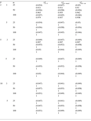
For ideal condition when g = 0 and h = 0 as shown in Table 1, all charts control on false alarms regardless of the number quality characteristics, p

and the sample sizes, m. This case represents the normal data where there is no problem in the controlling between the traditional and the robust charts. In this case the performance of the charts in term of the probability of detection and false alarm rate is good.

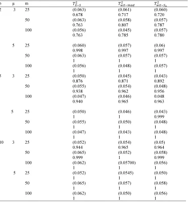
For the mild case when g= 0.5 and h = 0 as displayed in Table 2, the false alarm rates for the alternative Hotelling’s _{charts are better than the}

false alarm rates of the traditional Hotelling’s

_{charts. The rates are under control regardless of}

the number of characteristics of variables, p unlike the traditional chart, which deteriorates its control of false alarm when the number of characteristics of variables, p increases. Even the probabilities of detection non normal data for all the robust

_{charts are larger than the probability of detection}

non normal of the traditional _{charts. Moreover,}

the comparison between the ideal case as shown in Table 1and this case is important where the reader can note the performance of the robust charts in this case is stronger than the performance of the robust charts in ideal condition. Thus, in case of g = 0.5 an

h=0, the performance of the robust _{charts in}

terms of false alarm rates and probability of detection are considerably better than the traditional

charts.

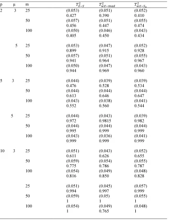
As shown in Table 3, when the values of g= 0 and h

(5)

219 tail are worse than with skewed (Table 2) in all of the control charts used.

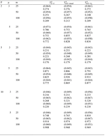
In Table 4, the results for the extreme case when

g=0.5 and h=0.25 (skewed and heavy tail) reveal that the alternatives charts outperform the traditional charts in term of false alarm. However, the rates of false alarms are in control when the sample size small while the rates of false alarms deteriorate as the sample sizes increase. The performance of the traditional and proposal control charts is worse in the case of lower changes in the means, that is when the mean is 3, because with this kind of distribution is more difficult to detect this out of control observations. Moreover, the performance is worse when there are few observations because in this case is more difficult for the charts to difference between in or out of control observations. However, in both cases the traditional chart generates very low probability of detection, while the robust charts could achieve stronger performance to detect the out of control observation.

As a result, in term of false alarms, it is noted that all charts work well when the sample sizes are small and deteriorate in its performance as the sample sizes increase. In addition, it is also noted in term of probability of detection all values are small and increase as the extreme non normal data increase.

6. REAL CASE STUDY.

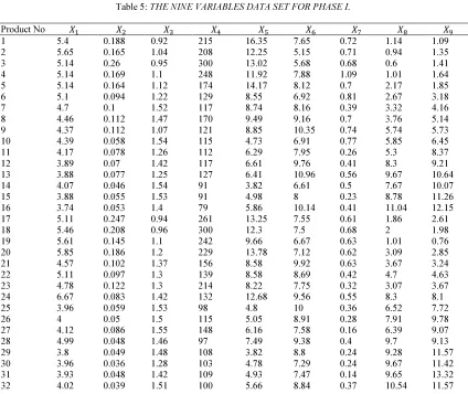
To investigate the performances for the two new robust Hotelling’s charts and compare them with the traditional Hotelling’s 2charts, we considered data about gilgaied soil available in the R package “MMST” as a real case to check the new robust charts. The data were used by Izenman (2008) and consist of data collected by the study of Horton, et al. [15] about nine variables for a sample of 48 soils. The nine variables are: Nitrogen percentage (X1); Bulk density (X1); Phosphorus in

ppm (X1); Calcium (X1); magnesium (X1);

potassium (X1); sodium (X1) and conductivity of

the saturation extract (X1). First of all, we have

verified that the data distribution is non normal. For this, we have used the Shapiro-Wilk Multivariate Normality Test available in the R package “mvnormtest” and the Mardia's and Royston's Multivariate Normality Tests available in the package “MVN” that verify that the data distribution is non normal. Therefore, we have used this data set to make comparison among the three charts the traditional and the two proposed

Hotelling’s 2 charts considering that the first 32 observations constitute the phase I data and the other 16 the phase II data. Table (5) contains the observations of the nine variables of phase I and Table (6) represents phase II of the nine variables for the production process with the values of the traditional and the two proposed Hotelling’s

2

statistics.

In order to determine the control limits that we must use in this real case, we have analysed the data performance in terms of skew and kurtosis. For this proposal, we have use the function “mardia” available in the package psych of R in order to determine the Mardia`s test for multivariate skew and kurtosis. The results obtained for this test with the data used in phase I verify that data has skewed with heavy tail and therefore we used the control limits for this case that they are 96.330; 245.263 and 192.876, for ̅ ; ̅ ! ̅ ,

respectively. Using these control limits, the results in table (6) show as the traditional control chart detect a signal in the observation number 9 but, however, using the robust alternatives proposal in this paper this observation is on control. Therefore, the use of robust alternatives in this situation with non normal data allows avoid the detection of one false alarm which is analyzed and in this case it is not necessary.

Moreover, if we do not analyze the data behavior and we use the control limits in normal case, which values are 28.789; 34.350 and 30.247, respectively, the three control charts consider this observation and the observation number 2 as observations out of control. Therefore, if the data behavior it is not considered the application of traditional and robust control charts make that the charts show a lot of false alarms. Thus, in the application of the robust control charts proposal in this paper it is very important firstly analyse the data performance in order to select the correct control limits and after applied these robust alternatives in order to avoid false alarm that it has cost for the industry.

7. CONCLUSION

This paper proposed two robust Hotelling's

control charts using winsorized MOM and winsorized covariance matrix as the location mean vector and scale covariance matrix, respectively. The default trimming criterion in MOM i.e.

was replaced with other highest breakdown points scale estimators, namely . The performance of

(6)

alarm and probability of detection of out of control non normal data. Investigations on the performance cover the cases of g=0 with h=0, g=0.5 with h=0,

g=0 with h=0.25 and g=0.5 with h=0.25. Simulation results show that the two robust

charts are in control of false alarm rates under most of the study conditions, but tend to lose control when the sample sizes increase. These robust charts are also able to generate probability of detection out of control non normal data better than the traditional chart, while they show decline when the number of the characteristics variables increase. Between the two robust charts, the chart

̅ has stronger performance in term of false

alarm and probability of detection outliers data.

8. FURTHER RESEARCHES

This study can be applied on many other types of simulation non normal data such as grouped data and data that are generated by using bootstrap method. This non normal data can be used by another robust location and scale estimators.

REFERENCES

[1] Abu-Shawiesh, M. O. & Abdullah, M., "A new Robust Bivariate Control Chart For Location". Communication in statistics,

Vol. 30, 2001, pp. 513 – 529.

[2] Alfaro, J. L., & Ortega, J. F., "A Robust Alternative to Hotelling’s T2 Control Chart UsingTrimmed Estimators". Qual. Reliab. Engng. Int., 24, 2008, pp. 601-611. [3] Alfaro, J. L., & Ortega, J. F., "A

comparison of robust alternative to Hotelling T^2 control chart", Applied Statistics, Vol. 36 No. 12, 2009, pp.1385-1396.

[4] Alfaro, J. L., & Ortega, J. F., "Robust Hotelling's T2 control charts under non-normality: the case of t-Student distribution". Journal of Statistical Computation and Simulation, Vol. 83, No. 10, 2012, pp. 1437-1447.

[5] Alfaro, J. L., & Ortega, J. F., "A new control chart in contaminated data of t-Student distribution for individual observations'. Applied Stochastic Models in Business and Industry, Vol. 29 No. 1, 2013, pp. 79-91.

[6] Alloway, J. A., & Raghavachari, M., "Multivariate Control Charts Based on Trimmed Mean. ASQC Quality Congress"

Transactions – San Francisco, 1990, pp. 449-453.

[7] Alloway, J. A., & Raghavachari, M., "An introduction to Multivariate Control Charts". ASQC Quality Congress Transactions – Milwaukee, 1991, pp. 773-781.

[8] Badrinath, S. G. & Chatterjee, S., "On Measuring Skewness and Elongation in Common Stock Return Distributions: The Case of the Market Index," Business, Vol. 61, No. 4, 1988, pp. 451-472.

[9] Badrinath, S. G. & Chatterjee, S., "A Data-Analytic Look at Skewness and Elongation in Common-Stock-Return Distributions,"Business and Economic Statistics, Vol. 9, No. 9, 1991, pp. 223-233.

[10] Cheng, L. M., Away, Y. & Hasan, M. K., "The Algorithm and Design of Real-time Multivariate Statistical Process Control System". Multimedia Cyberspace, Vol. 4, No. 2, 2006, pp. 18-23.

[11] Chenouri, S., Variyath, A., M, & Steiner, S. H., "A Multivariate Robust Control Chart for Individual Observations". Quality Technology, Vol. 41, No. 3, 2009, pp. 259-271.

[12] Chou, Y. M., Mason, R.L. & Young, J.C., "The Control Chart for Individual Obervations from A Multivariate Non-normal Distribution". Communications in Statistics - Simulation and Computation, Vol. 30, No. (8-9), 2001, pp. 1937-1949. [13] Haddad, F. S., Yahaya, S. S. & Alfaro, J.

L., "Alternative Hotelling T2 chart using Winsorized Modified One Step M-Esttimato". Quality and Reliability Engineering International, Vol. 29, No. 4, 2012, pp. 583-593

[14] Hoaglin, D. C., “Summarizing Shape Numerically: The g-and-h Distributions.” Chapter 11 in Exploring Data Tables Trends, and Shapes. Eds. Hoaglin, Mosteller, and Tukey. New York, NY: John Willey, 1985.

[15] Horton, I.F., Russell, J.S. & Moore, A.W., "Multivariatecovariance and canonical analysis: a method for selecting the most effective discriminators in a multivariate situation". Biometrics, Vol. 24, 1068, pp. 845-858.

(7)

221

Quality and Reliability Engineering International, 2006.

[17] Midi, H., Shabbak, A., Talib, B. A. & Hassan, M. N., "Multivariate control charts based on robust Mahalonobis distance". Paper presented at the Proceedings of the 5th Asian Mathematical Conference, Malaysia, 2009.

[18] Mills, T.C., "Modeling Skewness and Kurtosis in the London Stock Exchange FT-SE Index Return Distributions,"

Statistician, Vol. 44, No. 3, 1995, pp. 323-332

[19] Nedumaran, G., & Pignatiello, J. J., "On constructing T2 control charts for retrospective examination".

communication in Statistics-Simulation and Computation, Vol. 29, 2000, pp. 621-632.

[20] Pan, J. N. & Chen, S. C., "New Robust Estimators for Detecting Non-Random Patterns in Multivariate Control Charts: A Simulation Approach". Journal of Statistical Computation and Simulation, Vol. 81, No. 3, 2010, pp. 289-300. [21] Rousseeuw, P. J., & Croux, C., "Alternatives

to the Median Absolute Deviation. [Theory and Methods]". American Statistical Association, Vol. 88, No. 424, 1993.

[22] Sullivan, J. H. & Woodal, W. H., "A comparison of Multivariate Control Charts for Individual Observations". Quality Technology, Vol. 28, 1996, pp. 398 - 408. [23] Sun, R. & Tsung, F., “A kernel-distance-based multivariate control chart using support vector methods” International Journal of Production Research, Vol. 41, 2003, pp. 2975-2989.

[24] Surtihadi, J.,"Multivariate and robust control charts for location and dispersion".

Rensselaer’s School of Engineering, Rensselaer Polytechnic Institute, Troy, New York, U.S.A, 1994.

[25] Syed, S. S., Othman, A. R., & Keselman, H. J., "Comparing the Typical Score Across Independent Groups Based on Different Criteria for Trimming".

Metodoloski zvezki, Vol. 3, No. 1, 2006, pp. 49-62.

[26] Thissen, U., Swierenga, H.,Wehrens, R., Melssen, W.J., & Buydens, M.D., "Multivariate statistical process control using mixture modelling", Chemometrics,

Vol. 19, 2005, pp. 23–31.

[27] Vargas, J. A., "Robust Estimation in Multivariate Control Charts for Individual observation". Quality Technology, Vol. 35, 2003, pp. 367 - 376.

[28] Wilcox, R., & Keselman, H. J., "Repeated Measures ANOVA Based on a Modified One-Step M-Estimator". British Mathematical and Statistical Psychology, Vol. 56, No. 1, 2003, pp. 15 - 25.

(8)

APPENDIX

Table 1: (FALSE ALARM) AND THE PROBABILITY OF DETECTIONNON NORMAL DATA FOR THE TRADITIONALAND TWO ROBUSTCHARTS WHEN G=0, H=0.

P

2 3 m 25

50

100

̅

(0.054) 0.933 (0.056) 0.965 (0.047) 0.979

̅

(0.047) 0.931 (0.058) 0.955 (0.045) 0.957

̅

(0.05) 0.93 (0.056) 0.962 (0.046) 0.958

5 25 (0.054)

1

(0.047) 1

(0.05) 1

50 (0.056)

1

(0.058) 1

(0.056) 1

5 3

100

25

50

100

(0.047) 1

(0.049) 0.997 (0.055) 1 (0.05) 1

(0.045) 1

(0.047) 0.997 (0.052) 1 (0.044) 1

(0.046) 1

(0.049) 0.997 (0.058) 1 (0.049) 1

5 25 (0.049)

1

(0.047) 1

(0.049) 1

50 (0.055)

1

(0.052) 1

(0.058) 1

100 (0.05)

1

(0.044) 1

(0.049) 1

10 3 25

50

100

(0.047) 1 (0.057) 1 (0.051) 1

(0.041) 1 (0.055) 1 (0.049) 1

(0.049) 1 (0.058) 1 (0.049) 1

5 25 (0.047)

1

(0.041) 1

(0.049) 1

50 (0.047)

1

(0.055) 1

(0.058) 1

100 (0.051)

1

(0.049) 1

[image:8.595.113.485.182.676.2]

(9)

[image:9.595.116.488.178.579.2]

223

Table 2: (FALSE ALARM) AND THE PROBABILITY OF DETECTIONNON NORMAL DATA FOR THE TRADITIONALAND TWO ROBUSTCHARTS WHEN g=0.5, h=0.

p µ m ̅

̅

೙

2 3 25

50 100

(0.063) 0.678 (0.063) 0.763 (0.056) 0.763

(0.061) 0.717 (0.058) 0.807 (0.045) 0.785

(0.060) 0.720 (0.057) 0.787 (0.057) 0.780

5 25 (0.060)

0.998

(0.057) 0.997

(0.06) 0.997

50 (0.063)

1

(0.057) 1

100 (0.056)

1

(0.048) 1

(0.057) 1 5 3 25

50

100

(0.050) 0.876 (0.055) 0.938 (0.047) 0.940

(0.045) 0.871 (0.054) 0.962 (0.046) 0.965

(0.043) 0.892 (0.048) 0.956 0.048 0.963

5 25 (0.050)

1

(0.046) 1

(0.043) 0.999

50 (0.055)

1

(0.050) 1

(0.048) 1

100 (0.047)

1

(0.043) 1

(0.048) 1 10 3 25

50

100

(0.052) 0.944 (0.065) 0.999 (0.062) 1

(0.054) 0.965 (0.052) 1 (0.05700) 1

(0.05) 0.964 (0.058) 0.999 (0.056) 1

5 25 (0.052)

1

(0.0545) 1

(0.050) 1

50 (0.065)

1

(0.057) 1

(0.058) 1

100 (0.062)

1

(0.050) 1

(10)

[image:10.595.132.473.189.631.2]

Table 3: (FALSE ALARM) AND THE PROBABILITY OF DETECTIONNON NORMAL DATA FOR THE TRADITIONALAND TWO ROBUSTCHARTS WHEN g=0, h = 0.25.

p µ m ̅

̅

೙

2 3 25

50

100

(0.053) 0.427 (0.057) 0.456 (0.050) 0.405

(0.051) 0.390 (0.051) 0.447 (0.046) 0.450

(0.052) 0.410 (0.055) 0.474 (0.043) 0.434

5 25 (0.053)

0.899

(0.047) 0.915

(0.052) 0.928

50 (0.057)

0.941

(0.051) 0.964

(0.055) 0.967

100 (0.050)

0.944

(0.047) 0.969

(0.043) 0.960

5 3 25

50

100

(0.044) 0.476 (0.044) 0.613 (0.043) 0.552

(0.039) 0.528 (0.044) 0.646 (0.038) 0.560

(0.039) 0.534 (0.044) 0.647 (0.041) 0.544

5 25 (0.044)

0.972

(0.043) 0.9815

(0.039) 0.982

50 (0.044)

0.995

(0.044) 0.999

100 (0.043)

0.999

(0.036) 0.999

(0.041) 0.999

10 3 25

50

100

(0.051) 0.611 (0.059) 0.775 (0.054) 0.816

(0.043) 0.626 (0.054) 0.786 (0.049) 0.850

(0.052) 0.655 (0.055) 0.787 (0.048) 0.828

25 (0.051)

0.994

(0.045) 0.997

(0.057) 0.999

50 (0.059)

1

(0.05) 1

(0.055) 1

100 (0.054)

1

(0.049) 0.765

(11)

[image:11.595.122.483.157.620.2]

225

Table 4: (FALSE ALARM) AND THE PROBABILITY OF DETECTIONNON NORMAL DATA FOR THE TRADITIONALAND TWO ROBUSTCHARTS WHEN g=0.5, h=0.25.

P µ m ̅

̅

೙

2 3 25

50

100

(0.064) 0.274 (0.054) 0.251 (0.056) 0.209

(0.054) 0.276 (0.057) 0,267 (0.055) 0.213

(0.061) 0.272 (0.052) 0.248 (0.058) 0.209

5 25 (0.071)

0.786

(0.054) 0.753

(0.061) 0.765

50 (0.060)

0.753

(0.057) 0.855

(0.052) 0.837

100 (0.062)

0.772

(0.055) 0.828

(0.058) 0.830

5 3 25

50

100

(0.044) 0.231 (0.054) 0.221 (0.044) 0.170

(0.045) 0.253 (0.048) 0.268 (0.042) 0.179

(0.043) 0.223 (0.049) 0.281 (0.044) 0.179

5 25 (0.064)

0.871

(0.045) 0.806

(0.043) 0.791

50 (0.054)

0.825

(0.048) 0.920

(0.049) 0.933

100 (0.044)

0.775

(0.041) 0.869

(0.044) 0.877

10 3 25

50

100

(0.046) 0.216 (0.065) 0.268 (0.060) 0.220

(0.049) 0.211 (0.062) 0.321 (0.049) 0.239

(0.056) 0.233 (0.067) 0.320 (0.051) 0.230

5 25 (0.046)

0.748

(0.049) 0.765

(0.056) 0.810

50 (0.065)

0.914

(0.062) 0.974

(0.067) 0.973

100 (0.060)

0.908

(0.049) 0.968

(12)

[image:12.595.87.511.126.483.2]

Table 5: THE NINE VARIABLES DATA SET FOR PHASE I.

Product No

1 5.4 0.188 0.92 215 16.35 7.65 0.72 1.14 1.09

2 5.65 0.165 1.04 208 12.25 5.15 0.71 0.94 1.35

3 5.14 0.26 0.95 300 13.02 5.68 0.68 0.6 1.41

4 5.14 0.169 1.1 248 11.92 7.88 1.09 1.01 1.64

5 5.14 0.164 1.12 174 14.17 8.12 0.7 2.17 1.85

6 5.1 0.094 1.22 129 8.55 6.92 0.81 2.67 3.18

7 4.7 0.1 1.52 117 8.74 8.16 0.39 3.32 4.16

8 4.46 0.112 1.47 170 9.49 9.16 0.7 3.76 5.14

9 4.37 0.112 1.07 121 8.85 10.35 0.74 5.74 5.73

10 4.39 0.058 1.54 115 4.73 6.91 0.77 5.85 6.45

11 4.17 0.078 1.26 112 6.29 7.95 0.26 5.3 8.37

12 3.89 0.07 1.42 117 6.61 9.76 0.41 8.3 9.21

13 3.88 0.077 1.25 127 6.41 10.96 0.56 9.67 10.64

14 4.07 0.046 1.54 91 3.82 6.61 0.5 7.67 10.07

15 3.88 0.055 1.53 91 4.98 8 0.23 8.78 11.26

16 3.74 0.053 1.4 79 5.86 10.14 0.41 11.04 12.15

17 5.11 0.247 0.94 261 13.25 7.55 0.61 1.86 2.61

18 5.46 0.208 0.96 300 12.3 7.5 0.68 2 1.98

19 5.61 0.145 1.1 242 9.66 6.67 0.63 1.01 0.76

20 5.85 0.186 1.2 229 13.78 7.12 0.62 3.09 2.85

21 4.57 0.102 1.37 156 8.58 9.92 0.63 3.67 3.24

22 5.11 0.097 1.3 139 8.58 8.69 0.42 4.7 4.63

23 4.78 0.122 1.3 214 8.22 7.75 0.32 3.07 3.67

24 6.67 0.083 1.42 132 12.68 9.56 0.55 8.3 8.1

25 3.96 0.059 1.53 98 4.8 10 0.36 6.52 7.72

26 4 0.05 1.5 115 5.05 8.91 0.28 7.91 9.78

27 4.12 0.086 1.55 148 6.16 7.58 0.16 6.39 9.07

28 4.99 0.048 1.46 97 7.49 9.38 0.4 9.7 9.13

29 3.8 0.049 1.48 108 3.82 8.8 0.24 9.28 11.57

30 3.96 0.036 1.28 103 4.78 7.29 0.24 9.67 11.42

31 3.93 0.048 1.42 109 4.93 7.47 0.14 9.65 13.32

32 4.02 0.039 1.51 100 5.66 8.84 0.37 10.54 11.57

Table 6: THE NINE VARIABLES DATA SET WITH THE VALUES OF

STATISTIC USING THE TRADITIONAL ESTIMATORS AND THE TWO WINSORIZED MOM FOR PHASE II.

Product No

̅

[image:12.595.85.515.530.717.2]