The 22nd International Conference on Machine Learning
Proceedings of the Workshop on
Machine
Learning Techniques
for Processing
Multimedia Content
Matthieu Cord
Pádraig Cunningham
Rozenn Dahyot
Tamas Sziranyi
7-11 August 2005 in Bonn, Germany
Preface
Machine Learning (ML) techniques are used in situations where data is available in electronic format
and ML algorithms can ’add value’ by analysing this data. This is the situation with the processing of
multimedia content. The ’added value’ from ML can take a number of forms:
•
by providing insight into the domain from which the data is drawn,
•
by improving the performance of another process that is manipulating the data,
•
by organising the data in some way or
•
by helping to interpret multimedia content to make it more understandable.
This potential for ML to add value in processing of multimedia content has made this one of the most
popular application areas for ML research. Multimedia content has some characteristics that place
spe-cific demands on ML. The data is typically of very high dimension and dimension reduction is often
required. The normal distinction between supervised and unsupervised techniques doesn’t always
ap-ply; it is often the case that only some of the data is labeled or the user may assist in labeling the data
during processing. Typically the ML process is preceded by a feature extraction stage and the success
of the ML stage will often depend on the feature extraction.
This workshop on Machine Learning Techniques for Processing Multimedia Content has been
or-ganized because of these special issues that arise with multimedia data. We have papers describing
applications in image processing, video analysis and music classification. The research described in
these papers has drawn on a wide range of ML techniques. It is hoped that this workshop will help
iden-tify important research directions for Machine Learning that will help in the processing of multimedia
content.
We would like to express our thanks to the Programme Committee for their help in selecting the
papers for presentation at this workshop. Finally, we thank Hendrik Blokeel for his overall organization
of the 2005 ICML workshop series.
June 2005
Matthieu Cord
Pádraig Cunningham
Rozenn Dahyot
Tamás Szirányi
Workshop Organisation
Co- chairs
Matthieu Cord
Pádraig Cunningham
Rozenn Dahyot
Tamás Szirányi
Programme Committee
Horst Bischof, Graz University of Technology Austria
Matthieu Cord, ENSEA France
Pádraig Cunningham, Trinity College Dublin Ireland
Rozenn Dahyot, Trinity College Dublin Ireland
Christophe Garcia, France Telecom R&D France
Christophe Laurent, France Telecom R&D France
Nathalie Laurent, France Telecom R&D France
Shaul Markovitch, Technion Israel
Eric Moulines, ENST France
Eric Pauwels, CWI The Netherlands
Nicu Sebe, University of Amsterdam The Netherlands
Ovidio Salvetti, CNR Italy
Fred Stentiford, UCL United Kingdom
Tamás Szirányi, SZTAKI Hungary
Dietrich Wettschereck, Recommind Germany
Contents
Preface
1
Workshop Organisation
3
Contents
6
1
Motion Analysis and Synthesis of Time dependent Data, Hongyu Li, Wenbin Chen and
I-Fan Shen
7
2
Decision Trees and Random Subwindows for Object Recognition, Raphaël Marée, Pierre
Geurts, Justus Piater and Louis Wehenkel
13
3
Multimedia Target Tracking through Feature Detection and Database Retrieval, Maria
Grazia Di Bono, Gabriele Pieri and Ovidio Salvetti
19
4
Active Learning Techniques for User Interactive Systems: Application to Image Retrieval,
Philippe Henri Gosselin and Matthieu Cord
23
5
Ant-like mobile agents for Content-Based Image Retrieval in distributed databases, Arnaud
Revel, David Picard and Matthieu Cord
29
6
Learning Human Motion Patterns from Symmetries, László Havasi, Zoltán Szlávik, Csaba
Benedek and Tamás Szirányi
32
7
Addressing Partial Relevance in Image Retrieval through Aspect-Based Relevance
Learn-ing, Mark Huiskes
38
8
Blotch detection in archive film restoration by adaptive learning, Attila Licsár, Tamás Szirányi
and László Czúni
44
9
Music Classification with Partial Selection Based on Confidence Measures, Wei Chai and
Barry Vercoe
48
10 Interactive video retrieval based on multimodal dissimilarity representation, Eric Bruno,
Nicolas Moenne-Loccoz and Stéphane Marchand-Maillet
54
11 Large Margin Multiple Hyperplane Classification for Content-Based Multimedia Retrieval,
Serhiy Kosinov, Ivan Titov and St´ephane Marchand-Maillet
60
12 AdaBoost learning of shape and color features for object recognition, Thang V. Pham,
Arnold W. M. Smeulders and Sanne Ruis
63
13 A Bayesian Method for Automatic Landmark Detection in Segmented Images, Katarina
Domijan and Simon Wilson
69
Motion Analysis and Synthesis of Time-dependent Data
Hongyu Li [email protected]
Shanghai Key Laboratory of Intelligent Information Processing (IIPL),
Department of Computer Science and Engineering, Fudan University, Shanghai, 200433, China
Wenbin Chen [email protected]
Department of Mathematics, Fudan University, Shanghai, 200433, China
I-Fan Shen [email protected]
Su Yang [email protected]
Shanghai Key Laboratory of Intelligent Information Processing (IIPL),
Department of Computer Science and Engineering, Fudan University, Shanghai, 200433, China
Abstract
In this paper temporal local tangent space align-ment is proposed to deal with time-dependent data, such as video and motion capture data. It is an extension of local tangent space alignment, for short, LTSA, from spacial to temporal learn-ing. LTSA is a nonlinear dimension reduction method based on Euclidean distance. Temporal LTSA, however, is dependent on the continuity of time of input data. Another algorithmic improve-ment is made upon LTSA for mapping new data between the low- and high-dimensional spaces, which makes LTSA suitable in a changing, dy-namic environment. When temporal LTSA is ap-plied to time-dependent data, motion of objects underlying in such data can be carefully analyzed in a low-dimensional space. Motion decomposi-tion and synthesis can be further made for real applications.
1. Introduction
Time-dependent data are those data containing information about time continuity such as video and motion capture data. The variation of such data is related with time. The raw time-dependent data taken with cameras or other cap-turing devices are in general of very high dimensionality. In nature, however, only a few degrees of freedom play an important role in the process of real human or animal motion. For example, one of most prominent features of
Appearing in Proceedings of the workshop Machine Learning Techniques for Processing Multimedia Content, Bonn, Germany, 2005.
human walking is the periodicity. For the convenience of studying the periodicity, human motion can be described using one degree of freedom which cyclically varies with time. Thus dimension reduction is necessary.
Dimension reduction is a preprocessing step for analysis of high-dimensional time-dependent data and acts as an im-portant role to synthesize smoother and more continuous movement. Traditional methods to perform dimension re-duction are mainly linear, including principal component analysis and multidimensional scaling (Duda et al., 2001). Recently, a conceptually simple yet powerful method for nonlinear dimension reduction has been proposed in (Zhang & Zha, 2004): local tangent space alignment (LTSA). Its basic idea is that the global structure of a nonlinear manifold can be obtained from the interaction of overlapping local tangent spaces. LTSA is superior to another popular nonlinear mapping method, locally linear embedding (LLE) (Roweis & Saul, 2000) since the LTSA method is able to discover more useful degrees of freedom than the LLE method (Li et al., 2005).
Although the authors demonstrate their algorithm on a number of artificial and realistic data sets, there have as yet been few reports of application of LTSA. LTSA does not derive an explicit mapping function between the high-and low-dimensional spaces, therefore when new data ar-rive, we have to put all data together and compute again, i.e., LTSA is stationary with respect to data and lacks gen-eralization to new data. In this paper, this problem will be addressed. We propose a simple technique to map new data in the high- or low-dimensional space to another space, which makes LTSA suitable in a changing, dynamic envi-ronment. Besides, temporal LTSA (TLTSA) is specially proposed for dealing with time-dependent data where the
Motion Analysis and Synthesis of Time-dependent Data
measure of neighborhood selection is not Euclidean dis-tance, but time interval.
The remainder of the paper is divided into the following parts. In section 2 LTSA is briefly introduced and extended to adapt itself to a dynamic environment. Section 3 presents the temporal variation of LTSA. Some experimental results are presented in section 4. Finally, section 5 ends with some conclusions.
2. Local Tangent Space Alignment
Time-dependant data can be essentially considered as a se-quence of vectors. For example, a fraction of video is com-posed of many frames of images considered as points with coordinate vectors in a high-dimensional image space. Let us consider a set of input points with coordinate vec-tors X = {xi}ni=1 in R
m. Our aim is to obtain a set
of output vectorsY = {yi}ni=1 in a d-dimensional space where d < m. In this paper, we use local tangent space alignment (LTSA) to achieve this goal. It assumes that all data lie on or close to a nonlinear manifold and the global geometrical structure of this manifold can be learned by analyzing its overlapping local geometrical structure. It treats local tangent space of each point as such geometry and aligns those tangent spaces between the high- and low-dimensional spaces. The corresponding low-low-dimensional coordinatesY are discovered in the process of alignment.
2.1. Summary of LTSA
In this paper we will not discuss the derivation and proof for LTSA (For details, please refer to (Zhang & Zha, 2004)). Next we briefly describe how to extract low-dimensional coordinatesY from a set of high-dimensional dataX with LTSA.
1. Findknearest neighborsXi={xji}, j= 1, . . . , kfor
each pointxi, i= 1, . . . , n.
2. Extract the local geometrical information by calculat-ing thedlargest eigenvectorsg1, . . . , gdof the
corre-lation matrix(Xi−x¯ieT)T(Xi−¯xieT).eis a column
vector whose entries are all ones.x¯irepresents the
av-erage of the neighborhood ofxi,x¯i = 1kPjxji.Set
Gi= [e/
√
k, g1, . . . , gd].
3. Construct the alignment matrixBby locally summing as follows:
B(Ii, Ii)←B(Ii, Ii) +I−GiGTi, i= 1, . . . , n
with initialB = 0. I is ak×k identity matrix,Ii
denotes the set of indices for theknearest neighbors ofxi.
4. Compute thed+1smallest eigenvectors of B and pick up the eigenvector matrix[u2, . . . , ud+1]
correspond-ing to the 2nd tod+1st smallest eigenvalues. Set the global coordinates
Y = [y1, . . . , yn] = [u2, . . . , ud+1]T.
Note neighborhood selection (the first step of LTSA) to es-timate the local tangent space is very crucial to the success of this algorithm. In the simplest formulation of the algo-rithm, one identifies a fixed number of nearest neighbors, k, per data point, as measured by Euclidean distance. Fig.1 shows the selection of neighbors in a 3-D space. All data points discretely distribute on the surface of a ball. Yel-low squares surrounded with a black loop are 15nearest neighbors of xi. They together with xi compose a local
neighborhood ofxi. Two of tangent vectors atxi,T1and
T2, approximately span the tangent space ofxi.
Figure 1. The selection of nearest neighbors in the 3-D Euclidean space. Yellow squares surrounded with a black loop are15nearest neighbors ofxi.
Other criteria, however, can also be used to choose neigh-bors. For example, one can identify neighbors by choosing all points within a ball of fixed radius. One can also use locally derived distance metrics based on a priori knowl-edge such as class membership or time order, which deviate significantly from a globally Euclidean norm. In general, neighborhood selection in LTSA presents an opportunity to incorporate a priori knowledge.
2.2. Dynamic LTSA
The original LTSA is stationary with respect to the data, that is, it requires a whole set of points as an input in order to map them into the embedding space. When new data points arrive, the only way to map them is to pool both old and new points and return LTSA again for this pool. Therefore, the original LTSA lacks generalization to new data, it is not suitable in a changing, dynamic environment. Our attempt is to adapt LTSA to a changing situation where the data come incrementally point by point, and avoid an expensive eigenvector calculation for each new query,
Motion Analysis and Synthesis of Time-dependent Data
Figure 2. Successful recovery of a manifold of known structure using LTSA.
which is inspired from (Saul & Roweis, 2002; Kouroteva et al., 2002). Let a set of pointsX ={xi},i = 1, . . . , n,
as an original input to LTSA. After dimension reduction with LTSA, the projection of X to the embedding space can be discovered,Y ={yi},i= 1, . . . , n. In particular,
to compute the outputyn+1for a new arriving pointxn+1,
we can do the following. First look for the pointxjclosest
toxn+1amongX.Letyjbe the projection ofxjto the
em-beddding space. The derivation of LTSA reveals that the following equation is approximately true:
xj−x¯j≈Jf(yj−y¯j) =T(yj−y¯j),
whereT is a transformation matrix of sizem×d,x¯j and
¯
yj are respectively the mean ofknearest neighbors ofxj
andyj. The matrixT can be straightforwardly determined
as
T = (xj−x¯j)(yj−y¯j)+. (1)
where (·)+
represents the Moore-Penrose generalized in-verse of a matrix. Assumexjandxn+1lie close enough to each other (Note that input dataXmust be dense enough to sufficiently cover the whole surface of the embedded man-ifold, or else our method of generalization can not perform well), so the transformation matrixTofxjis applicable to
xn+1.yn+1can be obtained
yn+1= ¯yj+T+(xn+1−x¯j). (2)
A mapping from the embedding space to the input space can also be derived in the same manner.
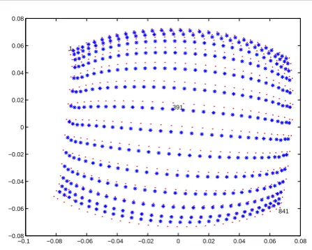
−0.1 −0.08 −0.06 −0.04 −0.02 0 0.02 0.04 0.06 0.08 −0.08
−0.06 −0.04 −0.02 0 0.02 0.04 0.06 0.08
1
[image:10.595.63.279.62.303.2]841 391
Figure 3. Mapping new arriving test images to the 2-D feature space learned from training images.
Let us consider 841 grayscale images of a single face trans-lated across a two-dimensional background shown in the top panel of Fig.2. Such images lie on an intrinsically two-dimensional nonlinear manifold in bottom panel, but have an extrinsic dimensionality equal to the number of pixels in each image (m=2576).
We divide the 841 images into two sets, which are alter-nately selected from left to right along the horizontal direc-tion. One set including 435 images is considered as original input data to learn a manifold, the other including 406 im-ages as new arriving data to test dynamic LTSA. Similar to the one using LTSA, the result using dynamic LTSA shown in Fig.3 successfully maps the images with corner faces to the corners of its two dimensional embedding and does re-flect the character of face movement. But dynamic LTSA only spends about 32.5 seconds on computation, which im-proves the efficiency by40%in comparison with 53.9 sec-onds that LTSA needs. Note the advantage of our method is not obvious when the test data set is too small, but when such set becomes very large, the computation efficiency will be greatly improved if using our method of general-ization .
3. Temporal LTSA
As stated in section 2.1, the criterion of neighborhood se-lection is supposed to the crucial feature of data sets. For time-dependent data, time order is more important than Eu-clidean distance, so in the process of neighborhood selec-tion, we can employ time order to decide the nearest neigh-bors of each point. This improved method is called tem-poral LTSA (TLTSA). For example, in Fig.5, if we take k= 5, the nearest neighbors of thei-th data along the time axis are those points betweeni−5-th andi+ 5-th.
Motion Analysis and Synthesis of Time-dependent Data
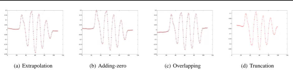
[image:11.595.65.536.57.171.2](a) Extrapolation (b) Adding-zero (c) Overlapping (d) Truncation
[image:11.595.78.262.228.267.2]Figure 4. Four feasible methods for dealing with margin points. a: the extrapolation method, b: the adding-zero method, c: the overlap-ping method, d: the truncation method.
Figure 5. The selection of nearest neighbors for time-dependent data.
For some points at the beginning and end of the sequence, their neighborhood is out of the sequence, thus the near-est neighbors can be chosen in some special ways. If not adding new data to the sequence, we can directly select some points near by them which may lead to the same neighborhood for some margin points. Or, we increase new data in order at the beginning and end of the sequence. New data can be same or not, for instance, they can be all-zero vectors; or extrapolate in terms of margin points to obtain new points. Another method is to give up those margin points to consider. In nature, all these methods have the similar effects.
Fig.4 presents four feasible methods for dealing with mar-gin points. This set of data taken with motion capture de-vices represent the walking motion of a human and will be in detail introduced in section 4.2. Since the walking mo-tion is approximately periodical, such data should essen-tially contain a significant degree of freedom which varies approximately periodically with time. The original data are of 54 dimensions, now we map them to a 1-D space with temporal LTSA. Four different methods are used for neighborhood selection of margin points. The extrapola-tion method first generates new data according to the origi-nal data and then inserts them on both sides of the sequence in order. The adding-zero method adds all-zero vectors on the outside of the sequence. The overlapping method does not introduce new data, it only admits margin points of a sequence to use the common neighborhood. The trunca-tion method directly gives up those margin points and only considered those points with applicable neighborhood. We have to again stress that the goal of the temporal LTSA algorithm is to obtain the global geometrical feature of a
set of data by the analysis of its local tangent space con-structed in terms of time order. Experimental results show that the algorithm is not sensitive for local discontinuity of data, i.e., adding/deleting some data to estimate local tan-gent spaces will not actually damage the character of the global geometry. In our following experiments, we will mainly use the overlapping method.
Besides, we have found that if the number of nearest neigh-bors k is set too small, the mapping will not reflect any global properties of data; if it is too high, the mapping will lose its nonlinear character and behave like traditional PCA, as the entire data set is seen as local neighborhood. The algorithm is stable over a wide range of values but do break down askbecomes too small or large.
4. TLTSA for Motion Analysis and Synthesis
In general, time-dependent data only can be shown by some special softwares or player. We can not directly take a com-plete view of their global continuity and smoothness. For better analyzing motion contained in time-dependent data, the TLTSA algorithm can be used to map these data to a lower-dimensional space (exactly 1-, 2- or 3-dimensional). Next we will respectively discuss two classes of time-dependent data, video and motion capture data, and present some experimental results.
4.1. Video Data
Video is composed of a sequence of images. If each im-age is represented by a vector, a section of video can be considered as a set of vector data with time order. Such data are high-dimensional, which is not beneficial for our direct analysis. When moving objects exist in a video, the vector data necessarily contain related motion infor-mation. Since most realistic movements such as walking, running and jumping are of low degrees of freedom, the high-dimensional vector data to represent this section of video contain a lot of redundant or insignificant informa-tion. Eliminating them can make it easy to study the mov-ing feature of such data. Here we apply the TLTSA
Motion Analysis and Synthesis of Time-dependent Data
[image:12.595.315.537.63.166.2]rithm into 35 face images (Fig.6) composing a section of discontinuous video about face rotation. A 2-D embedding was discovered by TLTSA and shown in Fig.7 where blue stars correspond to input training face images. Linear inter-polation is made between each pair of sequential points in the low-dimensional space and the results are represented by red points of Fig.7. By mapping those newly inserted points from the low- to high-dimensional spaces, one can obtain some new face images in the high-dimensional im-age space. Insert these new imim-ages back to the original image sequence, a section of new smooth video about face rotation can be generated.
Figure 6. 4 of 35 face images taken from different view angles – from side to frontal.
4.2. Motion Capture Data
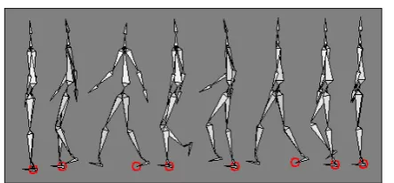
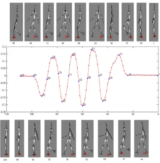
Motion capture data belong to another class of time-dependent data, which are widely applied in the field of character animation. Such data are not contaminated by the variation of background, therefore they can better embody the feature of motion than video data. Here we use a set of data with 54 dimensions representing walking of virtual hu-man (Fig.8) to analyze basic properties of huhu-man walking. Since human walking is or close to periodical, there should exist a degree of freedom describing such periodicity. Map such 109 continuous data to a 1-D space with TLTSA and show their variational regularity with time in Fig.9. Each red point corresponds to a walking state of virtual human and some key states corresponding to blue stars have be shown around the chart. Fig.9 reveals that the whole pro-cess of human walking can be approximately divided into three stages: the beginning (from Time 1 to Time 23), the circular advancement (from Time 24 to Time 99) and the ending (from Time 100 to Time 109). The advancement stage is composed of four primitive cycles. Extraction of the primitive motion from this stage allows us to arbitrar-ily copy such primitive and synthesize similar motion se-quences. That is, one can randomly assign the number of cycle and let virtual human smoothly walk in terms of the assigned number.
5. Conclusions
In this paper, we propose a simple technique to map new data in the high- or low-dimensional space to another space,
Figure 8. The walking process of virtual human which is used to capture motion data.
which makes LTSA suitable in a changing, dynamic envi-ronment. Besides, temporal LTSA is specially proposed for dealing with time-dependent data where the measure of neighborhood selection is not Euclidean distance, but time interval. Experiments show that the TLTSA algorithm can efficiently extract key degrees of freedom from time-dependent data, which is very beneficial for motion analy-sis and syntheanaly-sis.
Acknowledgments
This work was supported by NSFC under contract 60473104 and STCSM under contract 045115013.
References
Duda, R. O., Hart, P. E., & Stork, D. G. (2001). Pattern classification. New York, NY: John Wiley & Sons. 2 edition.
Kouroteva, O., Okun, O., Soriano, M., Marcos, S., & Pietikainen, M. (2002). Beyond locally linear embed-ding algorithmTechnical Report MVG-01-2002). Ma-chine Vision Group, University of Oulu, Finland. Li, H., Chen, W., & Shen, I.-F. (2005). Supervised
learn-ing for classification. ICNC’05-FSKD’05, LNCS (to ap-pear). Springer-Verlag.
Roweis, S., & Saul, L. (2000). Nonlinear dimension reduc-tion by locally linear embedding. Science, 290, 2323– 2326.
Saul, L., & Roweis, S. (2002). Think globally, fit locally: unsupervised learning of nonolinear manifoldsTechnical Report MS CIS-02-18). Univ. Pennsylvania.
Zhang, Z., & Zha, H. (2004). Principal manifolds and non-linear dimension reduction via local tangent space align-ment. SIAM Journal of Scientific Computing, 26, 313– 338.
Motion Analysis and Synthesis of Time-dependent Data
Figure 7. The mapping between the two- and high-dimensional spaces with TLTSA. Blue stars are generated from the input training face images. Red points are obtained by linear interpolation.
Figure 9. Periodicity of human walking. The horizontal axis represents the variation of time and gradually increases from right to left.
[image:13.595.134.463.356.691.2]Decision Trees and Random Subwindows for Object Recognition
Rapha¨el Mar´ee [email protected]
Pierre Geurts [email protected]
Justus Piater [email protected]
Louis Wehenkel [email protected]
Department of EE & CS, Institut Montefiore, University of Li`ege, B-4000 Li`ege, Belgium
Abstract
In this paper, we compare five tree-based machine learning methods within our recent generic image-classification framework based on random extraction and classification of subwindows. We evaluate them on three publicly available object-recognition datasets (COIL-100, ETH-80, and ZuBuD). Our com-parison shows that this general and concep-tually simple framework yields good results when combined with ensembles of decision trees, especially when using Tree Boosting or Extra-Trees. The latter is particularly at-tractive in terms of computational efficiency.
1. Introduction
Object recognition is an important problem within im-age classification, which appears in many application domains. In the object recognition literature, local approaches generally perform better than global ap-proaches. They are more robust to varying conditions because these variations can locally be modelled by simple transformations (Matas & Obdr˘z´alek, 2004). These methods are also more robust to partial occlu-sions and cluttered backgrounds. Indeed, the correct classification of all local features is not required to cor-rectly classify one image. These methods are generally based on region detectors (Mikolajczyk et al., 2005) and local descriptors (Mikolajczyk & Schmid, 2005) combined with nearest-neighbor matching.
In this paper, we compare five tree-based machine learning methods within the generic image classifi-cation framework that we proposed in earlier work (Mar´ee et al., 2005). It is based on random extraction
Appearing inProceedings of the workshop Machine Learn-ing Techniques for ProcessLearn-ing Multimedia Content, Bonn, Germany, 2005.
of subwindows (square patches) and their classification by decision trees.
2. Framework
In this section, we briefly describe the framework pro-posed by (Mar´ee et al., 2005). During the training phase, subwindows are randomly extracted from train-ing images (2.1), and a model is constructed by ma-chine learning (2.2) based on transformed versions of these (Figure 1). Classification of a new test image (2.3) similarly entails extraction and description of subwindows, and the application of the learned model to these subwindows. Aggregation of subwindow pre-dictions is then performed to classify the test image, as illustrated in Figure 2. In this paper, we evaluate various tree-based methods for learning a model.
2.1. Subwindows
The method extracts a large number of possibly over-lapping, square subwindows of random sizes and at random positions from training images. Each subwin-dow size is randomly chosen between 1×1 pixels and the minimum horizontal or vertical size of the current training image. The position is then randomly cho-sen so that each subwindow is fully contained in the image. By randomly selecting a large number (Nw) of subwindows, one is able to cover large parts of im-ages very rapidly. This random process is generic and can be applied to any kind of images. The same ran-dom process is applied to test images. Subwindows are resized to a fixed scale (16×16 pixels) and trans-formed to a HSV color space. Each subwindow is thus described by a feature vector of 768 numerical val-ues. The same descriptors are used for subwindows obtained from training and test images.
Decision Trees and Random Subwindows for Object Recognition ! ! " "# # $% &&& &&& &&& &&& ''' ''' ''' ''' ((( ((( ((( ((( ((( ))) ))) ))) ))) ))) *+ ,, ,, ,, ---- .. .. .. // // // 01 22222 22222 22222 33333 33333 33333 44 44 55 55 666 666 666 666 666 777 777 777 777 777 8 89 9 :: :: ;; ;; <=< <=< >=> >=>
C1 C2 C3
C1 C1 C1 C1 C2 C2 C2 C2 C2 C3 C3 C3 C3 C3 C1
T2
T1 T3 T4 T5
Figure 1.Learning: the framework first randomly extracts multi-scale subwindows from training-set images, then re-sizes them and builds an ensemble of decision trees.
2.2. Learning
At the learning phase, a model is automatically built using subwindows extracted from training images. First, each subwindow is labelled with the class of its parent image. Then, any supervised machine learning algorithm can be applied to build a subwindow classi-fication model. Here, the input of a machine learning algorithm is thus a training sample ofNwsubwindows, each of which is described by 768 real-valued input variables and a discrete output class (Figure 1). The learning algorithm should consequently be able to deal efficiently with a large amount of data, first in terms of the number of subwindows and classes of images in the training set, but more importantly in terms of the number of values describing these subwindows.
In this context, we compare five tree-based meth-ods: one single-tree method based on CART (Breiman et al., 1984), and four ensemble meth-ods: Bagging (Breiman, 1996), Boosting (Freund & Robert Schapire, 1996), Random Forests (Breiman, 2001), and Extra-Trees (Geurts, 2002). Extra-Trees only were originally used by (Mar´ee et al., 2005).
2.3. Recognition
In this approach, the learned model is used to classify subwindows of a test image. To make a prediction for a test image with an ensemble of trees grown from sub-windows, each subwindow is simply propagated into each tree of the ensemble. Each tree outputs condi-tional class probability estimates for each subwindow. Each subwindow thus receivesT class probability
es-T2
T1 T3 T4 T5
C1 C2 CM
0 4 0 0 00 1 0 00
C1 C2 CM
0 4 0 0 0 0 0 0 0 1
C1 C2 CM
?@?@? ?@?@? ?@?@? A@A A@A A@A B@B@B B@B@B B@B@B B@B@B C@C C@C C@C C@C D@D D@D D@D D@D E@E E@E E@E E@E F@F F@F G@G G@G H@H@H H@H@H H@H@H H@H@H I@I I@I I@I J JK K L@L@L L@L@L L@L@L M@M@M M@M@M M@M@M NONONON NONONON NONONON POPOPOP POPOPOP POPOPOP Q@Q@Q Q@Q@Q Q@Q@Q Q@Q@Q R@R R@R R@R SOSOS SOSOS TOT TOT U@U@U U@U@U U@U@U V@V@V V@V@V V@V@V W@W W@W W@W X@X X@X X@X Y Y Z Z [@[@[ [@[@[ [@[@[ [@[@[ [@[@[ \@\ \@\ \@\ \@\ \@\ ? ? ? ? ? ? ? + = C2
3 10 5
4
649 2 1 1 5
Figure 2.Recognition: randomly-extracted subwindows are propagated through the trees (hereT = 5). Votes are aggregated and the majority class is assigned to the image.
timate vectors where T denotes the number of trees in the ensemble. All the predictions are then aver-aged and the class corresponding to the largest aggre-gated probability estimate is assigned to the image. Note that we will simply consider that one single tree method is a particular case whereT = 1.
3. Experiments
Our experiments aim at comparing decision tree meth-ods within our random subwindow framework (Mar´ee et al., 2005). To this end, we compare these meth-ods on three well-known and publicly available object recognition datasets: household objects in a controlled environment (COIL-100), object categories in a con-trolled environment (ETH-80), and buildings in urban scenes (ZuBuD). The first dataset exhibits substantial viewpoint changes. The second dataset also exhibits higher intra-class variability. The third dataset con-tains images with illumination, viewpoint, scale and orientation changes as well as partial occlusions and cluttered backgrounds.
3.1. Parameters
For each problem and protocol, the parameters of the framework were fixed to Nw = 120000 learning
Decision Trees and Random Subwindows for Object Recognition
windows, T = 25 trees, and Nw,test = 100 subwin-dows are randomly extracted from each test image. In (Mar´ee et al., 2005), the parameters were fixed to
Nw = 120000, T = 10, and Nw,test = 100. Ensem-ble methods are influenced by the number of trees T
that are aggregated. Usually, the more trees are aggre-gated, the better the accuracy. We will further evalu-ate the influence of these parameters in Section 4.
For each machine learning method within the frame-work, the values of several parameters need to be fixed. In our experiments, single decision trees are fully de-veloped, i.e. without using any pruning method. The score used to evaluate tests during the induction is the score proposed by (Wehenkel, 1997) which is a particular normalization of the information gain. Oth-erwise our algorithm is similar to the CART method (Breiman et al., 1984).
Random Forests depends on an additional parameter
kwhich is the number of attributes randomly selected at each test node. In our experiments, its value was fixed to the default value suggested by the author of the algorithm which is the square root of the total number of attributes. According to (Breiman, 2001) this value usually gives error rates very close to the optimum.
With the latest variant of Extra-Trees (Geurts et al., 2005), the parameter k is the number of attributes randomly selected at each test node. We fixed it to the default value which is the square root of the total number of attributes. The main differences with Ran-dom Forests are that the algorithm ranRan-domizes also cut-point choice while splitting a tree node and grows the tree from the whole learning set while Random Forests uses bootstrap sampling.
Boosting does not depend on another parameter but it nevertheless requires that the learning algorithm does not give perfect models on the learning sample (so as to provide some misclassified instances). Hence, with this method, we used with decision trees the stop-splitting criterion described by (Wehenkel, 1997). It uses a hy-pothesis test based on the G2
statistic to determine the significance of a test. In our experiments, we fixed the nondetection riskαto 0.005.
3.2. COIL-100
COIL-1001
(Murase & Nayar, 1995) is a dataset of 128×128 color images of 100 different 3D objects (boxes, bottles, cups, miniature cars, etc.). Each ob-ject was placed on a motorized turntable and images were captured by a fixed camera at pose intervals of
1
http://www.cs.columbia.edu/CAVE/
Figure 3.COIL-100: some subwindows randomly ex-tracted from a test image and resized to 16×16 pixels.
5◦, corresponding to 72 images per object. Given a new image, the goal is to identify the target object in it.
On this dataset, reducing the number of train-ing views increases perspective distortions between learned views and images presented during testing. In this paper, we evaluate the robustness to viewpoint changes using only one view (the pose at 0◦) in the training sample while the remaining 71 views are used for testing. Using this protocol, methods in the lit-erature yield error rates from 50.1% to 24% (Matas & Obdr˘z´alek, 2004). Our results using this protocol (100 learning images, 7100 test images) are reported in Table 1. Tree Boosting is the best method for this problem, followed by Extra-Trees, Tree Bagging, and Random Forests. One decision tree has a higher er-ror rate. Examples of subwindows randomly extracted and resized to 16×16 pixels are given in Figure 3.
3.3. ETH-80
The Cogvis ETH-80 dataset2
contains 3280 color im-ages (128×128 pixels) of 8 distinct object categories (apples, pears, tomatoes, cows, dogs, horses, cups, cars). For each category, 10 different objects are pro-vided. Each object is represented by 41 images from different viewpoints.
In our experiments, we used for each category 9 objects in the learning set (8∗9∗41 = 2952 images), and the re-maining objects in the test set (8∗1∗41 = 328 images). We evaluate the methods on 10 different partitions, and the mean error rate is reported in Table 1. Here, Extra-Trees are slightly inferior while Tree Boosting and Tree Bagging are slightly better than other meth-ods.3
2
http://www.vision.ethz.ch/projects/ categorization/eth80-db.html
3
We observed that the adjustment of the extra-tree pa-rameterkto the half of the total number of attributes, in-stead of the square root, yields a 20.85% mean error rate. Such improvements might also be obtained for Random Forests.
Decision Trees and Random Subwindows for Object Recognition
Table 1.Classification error rates (in %) of all methods on COIL-100, ETH-80, ZuBuD (T = 25, Nw = 120000, Nw,test= 100)).
Methods COIL-100 ETH-80 ZuBuD
RW+Single Tree 19.20 22.04 10.43
RW+Extra-Trees 11.53 22.74 4.35
RW+R. Forests 13.06 21.31 4.35
RW+Bagging 12.77 20.34 3.48
RW+Boosting 10.75 20.27 3.48
3.4. ZuBuD
The ZuBuD dataset4
(Shao et al., 2003) is a database of color images of 201 buildings in Z¨urich. Each build-ing in the trainbuild-ing set is represented by five images acquired at five random arbitrary viewpoints. The training set thus includes 1005 images, while the test set contains 115 images of a subset of the 201 buildings. Images were taken by two different cameras in different seasons and under different weather conditions, and thus contain a substantial variety of illumination con-ditions. Partial occlusions and cluttered background are naturally present (trees, skies, cars, trams, people, . . . ) as well as scale and orientation changes due to the position of the photographer. Moreover, training images were captured at 640×480 while testing images are at 320×240 pixels.
About five papers have so far reported results on this dataset that vary from a 59% error rate to 0% (Matas & Obdr˘z´alek, 2004). Our results are reported in Table 1. Due to the small size of the test set, the difference between the methods is not dramatic and only one im-age makes the difference between the two best ensem-ble methods (Tree Boosting, Tree Bagging) and the two others (Extra-Trees and Random Forests). One single decision tree is again inferior. Figure 4 shows the 5 images misclassified by Extra-Trees and Ran-dom Forests, while the last one is correctly classified by Tree Boosting and Tree Bagging. For this last im-age, the correct class is ranked second by Extra-Trees and Random Forests.
4. Discussion
The good performance of this framework was ex-plained by (Mar´ee et al., 2005) by the combination of simple but well-motivated techniques: random
multi-4
http://www.vision.ee.ethz.ch/showroom/zubud/ index.en.html
Figure 4.ZuBuD: misclassified test images (left), training images of predicted class buildings (middle), training im-ages of correct buildings (right).
scale subwindow extraction, HSV pixel representation and recent advances in machine learning that have pro-duced new methods that are able to handle problems of high dimensionality.
For real-world applications, it may be useful to tune the framework parameters if a specific tradeoff be-tween accuracy, memory usage and computing times is desired. Then, in this section, we discuss the in-fluence of the framework parameters (4.1, 4.2, 4.3) on the ZuBuD problem which exhibits real-world images, and we present some complexity results (4.4).
4.1. Variation of Nw
Figure 5 shows that the error rate decreases monotoni-cally with number of learning subwindows (for a given number of trees (T = 25) and a given number of test subwindows (Nw,test= 100)). For all methods, we ob-serve that usingNw = 60000 subwindows already gives good results, and thatNw= 180000 does not improve accuracy, except for one single decision tree.
4.2. Variation of T
Figure 6 shows that the error rate decreases monoton-ically with the number of trees, for a given number of training subwindows (Nw = 120000) and test subwin-dows (Nw,test= 100). We observe that usingT = 10 trees is already sufficient for this problem for all en-semble methods.
Decision Trees and Random Subwindows for Object Recognition
0% 5% 10% 15% 20% 25% 30% 35% 40% 45%
0 60000 120000 180000
error rate (/115)
Nw
RW+Single Tree RW+Extra Trees RW+Random Forests RW+Bagging RW+Boosting
Figure 5.ZuBuD: error rate with increasing number of training subwindows.
2% 4% 6% 8% 10% 12% 14% 16% 18%
0 5 10 15 20 25
error rate (/115)
T
RW+Single Tree RW+Extra Trees RW+Random Forests RW+Bagging RW+Boosting
Figure 6.ZuBuD: error rate with increasing number of trees.
4.3. Variation of Nw,test
Figure 7 shows that the number of test subwindows also influences the error rate in a monotonic way, for a given number of training subwindows (Nw = 120000) and a given number of trees (T = 25). We observe that usingNw,test= 25 is already sufficient for this problem with ensemble methods, but the aggregation of more subwindows is needed for a single decision tree.
0% 10% 20% 30% 40% 50% 60% 70% 80% 90%
0 10 20 30 40 50 60 70 80 90 100
error rate (/115)
Nw,test
RW+Single Tree RW+Extra Trees RW+Random Forests RW+Bagging RW+Boosting
Figure 7.ZuBuD: error rate with increasing number of test subwindows.
4.4. Some notes on complexity
Our current implementation cannot be considered op-timal but some indications can be given about memory and running-time requirements. With this framework,
Table 2.ZuBuD: average tree complexity and learning time.
Methods Cmplx Learning Time
RW+Single Tree 92687 3h36m30s
RW+Extra-Trees 148080 14m05s
RW+Random Forests 77451 2h14m54s
RW+Bagging 63285 53h35m46s
RW+Boosting 28040 54h21m31s
original training images and their subwindows are not necessary to classify new images after the construction of the model, contrary to classification methods based on nearest neighbors. Here, only the ensemble of trees is used for recognition.
Learning times for one single decision tree and ensem-bles ofT = 25 trees are reported in Table 2, consider-ing that subwindows are in main memory. The com-plexity of tree-based method induction algorithm is of orderO(NwlogNw). Extra-Trees are particularly fast due to their extreme randomization of both attributes and cut-points while splitting a tree node. Single tree complexity (number of nodes) is also given in Table 2 as a basic indication of memory usage.
To classify a new image, we observed that the predic-tion of one test subwindow with one tree requires on average less than 20 tests (each of which involves com-paring the value of a pixel to a threshold), as reported in Table 35
. The minimum and maximum depths are also given. To classify one unseen image, the num-ber of operations is thus multiplied byT, the number of trees, and by Nw,test, the number of subwindows extracted. The time to add all votes and search the maximum is negligible. Furthermore, extraction of one subwindow is very fast because of its random nature.
On this problem, we have also observed that pruning Extra-Trees could substantially reduce their complex-ity (downto a tree complexcomplex-ity average of 25191 with the same stop-splitting criterion as Tree Boosting, thus giving an average test depth of 15.4) while keeping the same accuracy. In practical applications where pre-diction times are essential, the use of pruning is thus certainly worth exploring.
5
The average tree depth was calculated empirically over the 287500 propagations (100 subwindows for each of the 115 test images, propagated throughT = 25 trees), except for one single decision tree and for Tree Boosting (because the algorithm stopped afterT = 21 trees).
Decision Trees and Random Subwindows for Object Recognition
Table 3. ZuBuD: average subwindow test depth.
Methods Depth min max
RW+Single Tree 16.59 9 29
RW+Extra-Trees 18.26 8 34
RW+Random Forests 16.44 7 33
RW+Bagging 15.98 8 34
RW+Boosting 15.04 6 28
5. Conclusions
In this paper, we compared 5 tree-based machine learning methods within a recent and generic frame-work for image classification (Mar´ee et al., 2005). Its main steps are the random extraction of subwindows, their transformation to normalize their representation, and the supervised automatic learning of a classifier based on (ensembles of) decision tree(s) operating di-rectly on the pixel values. We evaluated the tree-based methods on 3 publicly-available object recog-nition datasets. Our study shows that this general and conceptually simple framework yields good results for object recognition tasks when combined with en-sembles of decision trees. Extra-Trees are particularly attractive in terms of computational efficiency dur-ing learndur-ing, and are competitive with other ensem-ble methods in terms of accuracy. This method with its default parameter allows to evaluate very quickly the framework on any new dataset.6
However, if the main objective of a particular task is to obtain the best error rate whatever the learning time, Tree Boosting appears to be a better choice. Tuning the parameters (such as the value of k in Extra-Trees, or the stop-splitting criterion) might further improve the results.
For future work, it would be interesting to perform a comparative study with SVMs. The framework should also be evaluated on bigger databases in terms of the number of images and/or classes and with images that exhibit higher intra-class variability and heavily clut-tered backgrounds (such as the Caltech-1017
, Birds, or Butterflies8
datasets).
6. Acknowledgment
Rapha¨el Mar´ee is supported by GIGA-Interdisciplinary Cluster for Applied Genoproteomics, hosted by the University of Li`ege. Pierre Geurts is
6
Java implementation is available for evaluation at http://www.montefiore.ulg.ac.be/~maree/
7
http://www.vision.caltech.edu/feifeili/ Datasets.htm
8
http://www-cvr.ai.uiuc.edu/ponce_grp/data/
a Postdoctoral Researcher at the National Fund for Scientific Research (FNRS, Belgium).
References
Breiman, L. (1996). Bagging predictors. Machine Learning,24, 123–140.
Breiman, L. (2001). Random forests. Machine learn-ing,45, 5–32.
Breiman, L., Friedman, J., Olsen, R., & Stone, C. (1984). Classification and regression trees. Wadsworth International (California).
Freund, Y., & Robert Schapire, E. (1996). Experi-ments with a new boosting algorithm. Proc. Thir-teenth International Conference on Machine Learn-ing(pp. 148–156).
Geurts, P. (2002). Contributions to decision tree in-duction: bias/variance tradeoff and time series clas-sification. Doctoral dissertation, Department of Electrical Engineering and Computer Science, Uni-versity of Li`ege.
Geurts, P., Ernst, D., & Wehenkel, L. (2005). Ex-tremely randomized trees. Submitted.
Mar´ee, R., Geurts, P., Piater, J., & Wehenkel, L. (2005). Random subwindows for robust image clas-sification. Proc. IEEE International Conference on Computer Vision and Pattern Recognition (CVPR). Matas, J., & Obdr˘z´alek, S. (2004). Object recognition methods based on transformation covariant features. Proc. 12th European Signal Processing Conference (EUSIPCO 2004). Vienna, Austria.
Mikolajczyk, K., & Schmid, C. (2005). A performance evaluation of local descriptors. PAMI, to appear. Mikolajczyk, K., Tuytelaars, T., Schmid, C.,
Zisser-man, A., Matas, J., Schaffalitzky, F., Kadir, T., & Gool, L. V. (2005). A comparison of affine region de-tectors. International Journal of Computer Vision, to appear.
Murase, H., & Nayar, S. K. (1995). Visual learning and recognition of 3d objects from appearance. In-ternational Journal of Computer Vision,14, 5–24. Shao, H., Svoboda, T., & Van Gool, L. (2003).Zubud
-Zurich building database for image based recognition (Technical Report TR-260). Computer Vision Lab, Swiss Federal Institute of Technology, Switzerland.
Wehenkel, L. A. (1997).Automatic learning techniques in power systems. Kluwer Academic Publishers, Boston.
Multimedia Target Tracking through Feature Detection and Database Retrieval
Maria Grazia Di Bono [email protected]
Gabriele Pieri [email protected]
Ovidio Salvetti [email protected]
Institute of Information Science and Technologies, ISTI-CNR, Via Moruzzi 1, 56124 Pisa, ITALY
Abstract
The real-time detection and tracking of moving objects is a challenging task and automatic tools to identify and follow them are often subject to constraints regarding the environment under investigation or the full visibility of the targeted object. Exploiting the possibility of a multi-source acquisition in the targeted scene, firstly detection is performed by means of characteristic features extraction and storing in a database; secondly, the tracking task is approached using algorithms, where automatic search involves occluded or masked targets in the scene. This latter problem is solved through database retrieval, based on well-defined multi-modal features. The method has been tested on case studies regarding the identification and tracking of animals moving at night in an open environment (i.e. natural reserves or parks), and the surveillance of known scenes for unauthorized access control.
1.
Introduction
According to the cognitive processes of the human perception (Milner & Goodale, 1995), a methodology has been developed which provides a way to realize object recognition and tracking in 3D real environments. In particular, this approach is based on the acquisition of multi-source information that is firstly elaborated for object detection and characterization, and then for its localization and active tracking. After target detection is achieved through an automatic segmentation, the characterization phase is performed through the description of multi-modal features (morphological, densitometric and semantic), which are extracted from the acquired multi-source information. Localization is realized using also features previously extracted and
stored in a reference database. In order to improve the localization performance when only partial information is available (i.e. in case of lost or occluded targets), the implemented method is supported by a content-based retrieval (CBR) paradigm using an a priori defined multimedia (MM) database. This MM database is built using the multi-modal features extracted from a set of target examples organised on the basis of semantic classes defined on the specific environment under investigation.
—————
Appearing in Proceedings of the workshop Machine Learning Techniques for Processing Multimedia Content, Bonn, Germany, 2005.
Current approaches regarding real-time object tracking from videos are based on (i) successive frame differences (Fernandez-Caballero et al., 2003), using also adaptive threshold techniques (Fejes & Davis, 1999), (ii) trajectory tracking, using weak perspective and optical flow (Yau, Fu & Liu, 2001), (iii) region approaches, using active contours of the target and neural networks for movement analysis (Tabb et al., 2002), or motion detection and successive regions segmentation (Kim & Kim, 2003).
Regarding the CBR paradigm, techniques of shape retrieval in large databases are particularly interesting. Considering a shape of an object as a sequence of contour points, a method using both global and local features is discussed in (Wang, Yang & Acharya, 1998) while in (Wang, Chang & Acharya, 1999) retrieval is based on a hash table and a majority voting algorithm for an efficient estimation of shape similarity. Furthermore, another interesting approach considers a shape database structured as an M-tree of organised tokens, representing parts of the shape enclosed between contour points. Possible shapes are clustered into semantic classes, each belonging to an object typology defined in its environment (Berretti, Del Bimbo & Pala, 2000).
In this paper, the problem of moving target detection and tracking is faced by processing multi-source information acquired using cameras of different typology (Far-IR and visible). Object characterization is based on region segmentation and feature extraction processes. Object localization uses a CBR approach based on similarity functions defined for each multi-modal feature class.
The method has been applied to real case studies regarding the monitoring of animal movements during the night in an open environment (i.e. natural reserves or parks) and the surveillance of known scenes for
Multimedia Target Tracking through Feature Detection and Database Retrieval
unauthorized access control in both open and closed spaces (Pieri et al., 2004).
2.
Problem definition
The precise identification of a defined target in a real video, frame by frame, is approached. The proposed methodology is based on recognition and spatial localization of the target: recognition is sub-divided into identification and characterization, while the spatial localization performs active tracking.
The multi-source information is acquired using a physical system composed of a thermo-camera and two stereo visible-cameras synchronized. Thus, we obtain a set of infrared (IR) images, which make the system more robust and invariant to light changes in the scene, corresponding to stereo grey level images.
A procedure has been defined based on two different stages:
Off-line stage, in which the recognition phase is performed using selected examples belonging to a set of predefined semantic classes, in order to populate the reference MM database.
On-line stage, in which the tracking is performed by applying recognition and spatial localization.
In deep details, during the recognition process, the identification phase consists of an automatic segmentation, based on edge detection using a gradient descent along 16 directions starting from a reference point internal to the target (centroid).
In the characterization phase, for each frame, the multi-source information is used in order to extract a target description from the scene. This is made through a feature extraction process performed on the three different images available for each frame in the sequence. In particular, the extraction of a depth index from the grey level stereo images, performed by computing disparity of the corresponding stereo points, is realized in order to have significant information about the target spatial localization in the 3D scene and the target movement along depth direction, which is useful for the determination of a possible static or dynamic occlusion of the target itself in the observed scene. Other features consisting in radiometric parameters measuring the temperature and visual features are extracted from the IR images. The visual features, grouped in morphological, densitometric and semantic classes, consist of shape contour descriptors, dominant colour discriminants, statistical parameters, computed on the regions enclosed by the contours (area, perimeter, average brightness, standard deviation, skewness, kurtosis, and entropy) and the semantic class to which the target belongs (i.e. human, small, medium and large animal, …). While the depth index and the visual features are automatically extracted from the images, the semantic classes of the observed
targets are selected by the user among a predefined set of possible choices.
During the off-line stage, all the multi-modal feature information is stored in the MM database, organised on the base of semantic classes. This information is used during the on-line spatial localization process, in particular in the automatic target retrieval which acts as a support during the active tracking in case of partial occlusion or quickly direction changes of the target.
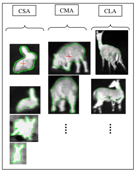
For each defined target class, possible variations of the initial shape, taking into account that the target could be still partially masked or have a different orientation, are recorded together with the other multi-modal features as it is shown in Figure 1.
[image:21.595.303.520.268.541.2]
Figure 1. Example of actual targets in the MM data-base, grouped according to the classes “small animal” (CSA), “medium animal” (CMA) and “large animal” (CLA).
During the on-line spatial localization, the extracted features drive tracking and also support CBR to resolve the queries to the MM database.
The first phase of the on-line stage is the same of the off-line one. An automatic segmentation of the target is performed on both the IR and stereo grey-level images, in order to characterize the selected target. Contextually, the user performs also the selection of the semantic class to which the target belongs.
CSA CMA CLA
Multimedia Target Tracking through Feature Detection and Database Retrieval
The tracking algorithm is performed on the IR image sequence, in order to build a system which can be used both at night and daylight.
The segmented target from the first IR image of the sequence is then tracked automatically in the following frame. The features used for the automatic tracking are local maxima, movement prediction (on the basis of the movements of the previous steps), temperature and a priori knowledge about the specific class the object belongs to. For each frame, the algorithm performs the steps to correctly identify the target and to follow it.
Firstly, a candidate characterizing point P1 of the target is selected in its centroid, in the actual frame. The selection follows criteria of brightness local maximum, inside the contour segmented in the previous frame; P1 is the point having the maximum similarity with the centroid PP of the previous frame.
In a second step, the algorithm takes into account the previous movements of the centroid. The trajectory is stored and then used in the computation of the actual step, locating a new candidate point P2. If P2 is not coincident with P1 then a new point P3 is calculated as:
3 1 2
P =αP+βP (1)
where and represent the weight assigned, and . These parameters are empirically defined and can be adjusted by the user.
α
β
1
=
β
+
α
Again, a local maximum search is performed in the neighbourhood of P3 to make sure that it is internal to a valid object. This search finds the point PN that has the grey level closest to the one of PP, so that PN is the centroid chosen for the actual frame. Starting from this point, the edge detection is performed and the object new contour is segmented.
In each frame, a first control is made trying to avoid a wrong object recognition, due to either a masking, partial occlusion of the object in the scene or to a quick movement in an unexpected direction. This control takes into account the above mentioned statistical parameters computed on the region enclosed by the contour, without using CBR paradigm in order to optimise the number of accesses to the database. If there are parameters exceeding p times (p is defined a priori) the standard deviation of the same parameters computed over the last n frames, the database search for the correct target is started. This search is based on the CBR paradigm; the multi-modal features of the candidate target are compared to the ones recorded in the MM database. A similarity function is considered for each feature class. In particular, we used similarity functions, as in (Tzouveli et al., 2004), for colour matching, using percentages and colour values, and shape matching, using the cross-correlation criterion. In order to obtain a global similarity measure, each similarity percentage is associated to a pre-selected weight, using the reference semantic class as a filter to access the MM information. If after j frames the correct
target has not yet been grabbed, the control is given back to the user. The value of j is computed considering the distance between PP and the edge point of the image along the search direction, divided by the average velocity of the target previously measured in the last n frames (Eq. 2).
Dist( P; r) / Vel
j= P E (2)
where Dist( , )x y is the Euclidean distance between points x and y; Er is the point crossing the edge of the frame
along the search direction r determined by the last n centroids; and Vel is
(3)
1
1
0
Vel Dist( ; ) /
n
i i P P i
P P n
−
+
=
⎛ ⎞
= ⎜⎜ ⎟⎟
⎝
∑
⎠where
P
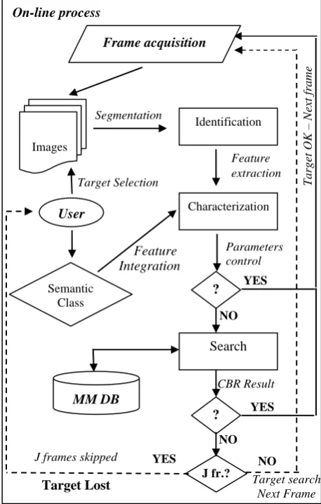
Pi is the centroid i steps before the actual. [image:22.595.300.529.321.680.2]The sketch of the methodology described is shown in Figure 2.
On-line process
Figure 2. Recognition and description of a target object (on-line process).
Images
User
Identification
MM DB Semantic
Class
Frame acquisition
T
a
rg
et OK – Ne
xt
fr
ame
Target Lost
J frames skipped Target Selection
CBR Result
Characterization
Search Feature
Segmentation
Integration
Target search Next Frame Feature extraction
Parameters control
YES ?
NO
YES ?
NO
YES NO
J fr.?
Multimedia Target Tracking through Feature Detection and Database Retrieval
3.
Results and Conclusions
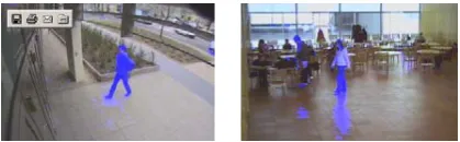
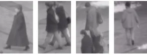
The method implemented has been applied to real case studies: (i) to track animal movements in an open environment during the night, for the fauna monitoring in natural parks, and (ii) for video surveillance of known scenes both at night and daylight to control unauthorized access (see Figure 3).
Figure 3. Examples of thermo images regarding human (left and centre, two different views and shapes) and animal (right) targets (crosses are the centroids).
Regarding the first case, due to the environmental conditions, only the thermo-camera has been used.
The videos were acquired using a thermo-camera in the 8-12µm wavelength range, mounted on a moving structure covering 360° pan and 90° tilt, and equipped with 12° and 24° optics to have 320x240 pixel spatial resolution.
Both the thermo-camera and the two stereo visible-cameras have been positioned in order to explore a scene 100 meters far, sufficient in our experimental cases.
In the fauna monitoring experimental case, during the off-line stage, the MM database has been built taking into account different image sequences relative to different classes of the monitored animals. In particular, three main semantic classes have been determined. The large-animal class counting all the monitored animals of a large size like deer, the medium-animal class including animals of medium size like boars and the small-animal class considering other kind of animals like rabbits or badgers. For each outlined semantic class, different positions have been considered. In more details, four different positions for boars, rabbits and other small animals and six for deer have been registered.
In the video-surveillance case, the human class has been composed taking into account six different pose conditions for three different people typology.
The acquired images are pre-processed to reduce the noise, the algorithm has shown an effective performance and seems promising in the lights of further improvements regarding for example the integration with audio information, coming from different aligned
microphones installed in the scene, and aiming at the same direction of the cameras.
References
Berretti, S., Del Bimbo, A., & Pala, P. (2000). Retrieval by Shape Similarity with Perceptual Distance and Effective Indexing. IEEE Transactions on Multimedia, 2 (4), 225–239.
Fejes, S., & Davis, L.S. (1999). Detection of Independent Motion Using Directional Motion Estimation. Computer Vision and Image Understanding, 74 (2), 101–120.
Fernandez-Caballero, A., Mira, J., Fernandez, M.A., & Delgado, A.E. (2003). On motion detection through a multi-layer neural network architecture. Neural Networks, 16, 205–222.
Kim, J.B., & Kim, H.J. (2003). Efficient region-based motion segmentation for a video monitoring system. Pattern Recognition Letters, 24, 113–128.
Milner, A.D., & Goodale, M.A. (1995). The Visual Brain in Action. Oxford: Oxford University Press.
Pieri, G., Benvenuti, M., Carnier, E., & Salvetti, O. (2004). Object detection and tracking in an open and free environment with a moving camera. Proceedings of Seventh International Conference on Pattern Recognition and Image Analysis: New Information Technologies (Vol. II, pp. 347–350), St. Petersburg, Russia, 18-23 October 2004.
Tabb, K., Davey, N., Adams, R., & George, S. (2002). The recognition and analysis of animate objects using neural networks and active contour models. Neurocomputing, 43, 145–172.
Tzouveli, P., Andreou, G., Tsechpenakis, G., Avrithis, Y., & Kollias, S. (2004). Intelligent Visual Descriptor Extraction from Video Sequences. Lecture Notes in Computer Science – Adaptive Multimedia Retrieval, 3094, 132–146.
Wang, J., Yang, W.-J., & Acharya, R. (1998). Efficient Access to and Retrieval from a Shape Image Database. Proceedings of the IEEE Workshop on Content-Based Access of Image and Video Libraries (pp. 63–67). Santa Barbara, CA.
Wang, J., Chang, W., & Acharya, R. (1999). Efficient and Effective Similar Shape Retrieval. Proceedings of the IEEE International Conference on Multimedia Computing and Systems (Vol. 1, pp. 875–879), Florence, Italy.
Yau, W.G., Fu, L.-C., & Liu, D. (2001). Robust Real-time 3D Trajectory Tracking Algorithms for Visual Tracking Using Weak Perspective Projection. Proceedings of the American Control Conference, Arlington, VA.
Active Learning Techniques for User Interactive Systems:
Application to Image Retrieval
Philippe Henri Gosselin [email protected]
Matthieu Cord [email protected]
ETIS / CNRS UMR 8051, 6 avenue du Ponceau, 95014 Cergy-Pontoise, France
Abstract
Active learning methods have been consid-ered with an increasing interest for user inter-active systems. In this paper, we propose an efficient active learning scheme to deal with this particular context. An active boundary correction is proposed in order to deal with few training data. Experiments are carried out on the COREL photo database.
1. Introduction
Human interactive systems has attracted a lot of re-search interest in recent years, especially for content-based image retrieval systems. Contrary to the early systems, focused on fully automatic strategies, re-cent approaches introduce human-computer interac-tion (Veltkamp, 2002; Vasconcelos & Kunt, 2001).
Starting with a coarse query, the interactive process allows the user to refine his request as much as neces-sary. Many kinds of interaction between the user and the system have been proposed (Chang et al., 2003), but most of the time, user information consists of bi-nary annotations (labels) indicating whether or not the image belongs to the desired category.
In this paper, we focus on the retrieval of concepts within a large document collection. We assume that a user is looking for a set of documents, the query concept, within an existing document database. The aim is to build a fast and efficient strategy to retrieve the query concept.
Performing an estimation of the query concept can be seen as a statistical learning problem, and more pre-cisely as a binary classification task between the rele-vant and irrelerele-vant classes (Chapelle et al., 1999). The
Appearing inProceedings of the workshop Machine Learn-ing Techniques for ProcessLearn-ing Multimedia Content, Bonn, Germany, 2005.
relevant class is the set of documents within the query concept, and the irrelevant class the set of documents out of the query concept. This context defines a very specific learning problem with the following character-istics:
1. High dimensionality. The documents used to be represented by vectors of high dimensionality.
2. Few training data. At the beginning, the system has to perform a good estimation of the query con-cept with very few data. Furthermore, the system can not ask user to label thousands of documents, good performances are required using a small per-centage of labeled data.
3. Relevance feedback. Due to user annotations, the training data set grows step by step during the retrieval session, so the current classification de-pends on the previous ones.
4. Unbalanced classes. The query concept is often a small subset of the database (some hundreds of documents). Thus, the relevant and irrelevant classes are highly unbalanced (up to factor 100), on the contrary to classical classification prob-lems, where the classes have approximatively the same size.
5. Limited computation time. The user can not wait several hours between each feedback steps. We as-sume that a user can wait at most several minutes between each feedback steps.
In this paper, we propose an active learning strategy to deal with these characteristics. In section 2, we present current methods for classification, and motiva-tions for active learning. In section 3, we focus on ac-tive learning, and present two well-known approaches: uncertainly-based sampling and error reduction. In section 4, we propose an active learning scheme to en-hance the previous methods. In section 5, experiments