Efficient Noise Removing based Optimized Smart
Dynamic Gaussian Filter
Hassen Seddik
Ezzedine Ben Braiek
ESSTT, 5 Av. Taha Hussein, 1008, Tunis, Tunisia ESSTT, 5 Av. Taha Hussein, 1008, Tunis,
ABSTRACT
Gaussian filter has been used extensively in signal image processing for many years. Gaussian or Gaussian derivative filtering is in several ways optimal for applications requiring low-pass filters or running averages. In this paper, a highly efficient noise removing technique based on a modified dynamic Gaussian filter is introduced. Called smooth filter, the Gaussian filter is known to be more efficient for conserving details and slight borders then other filters. In the proposed approach, we developed a variable shape low pass filter that can be used for efficient noise removal even with impulsive noise. In this study, the filter selects automatically the processed windows based on an automatic noise targeting in such a way that the image does not lose its characteristics. An optimal magnitude and support extent of the Gaussian filters is continually computed in an iterative method for each selected windows of the image. This approach is approved experimentally using salt and pepper noise. In fact Gaussian filter is not appropriate for removal of impulsive (salt and pepper) noise that needs filters based on statistical approach. Nevertheless high efficiency in removing high densities of noise difficult to remove even using median filter is shown. In addition the image quality is preserved. This proposed method combines the behavior of an intelligent dynamic low-pass filter that eliminates only high frequencies corresponding to noise and a filter based statistical approach such as median filter that removes efficiently impulsive noise and conserves details.
Keywords
: Efficient noise removing, Gaussian filter with dynamic structure targeted filtering.1. INTRODUCTION
Gaussian filters have held a fundamental role in image filtering because of research in human vision models [1], noise reduction [2], edge detection [1]...etc. In this work we are interested by low-pass filtering for de-noising purpose. In this context, we typically wish to attenuate high-frequencies corresponding to noise. In fact during the last few decades, Gaussian Kernel smoothing has been widely used in signal and image processing to improve the signal to noise ratio. Different representations have been proposed such as the anisotropic Gauss filtering by J.M. Geusenbraek [1], the multi-scale approach by M. Cheriet [3] and scale-space representation by Witkin [4] and Koendrink [5]. Witkin described the scale-space representation in terms of successive convolutions of the original image with Gaussian of increasing width [6]. Koenderink showed that the Gaussian space is equivalent to solving the linear diffusion equation [3]. Today the Gaussian filter has become a standard tool in low level image analysis. In the continuous Gaussian space, the implementation of a Gaussian filter in one or more dimension is applied as a convolution by the samples of the Gaussian function as shown
gn f k ngk
n f
(2)
Where
2 2 2 21
x n
x exp
n / x g n
g (3)
With is real and the size of the filter is limited to the window
N,N
instead of
,
, N is an integer chosen approximately such as N
6 .Fig. 1: one dimensional profile of the Gaussian kernel
The Gaussian kernel has some properties that make it unique [3] such as the semi-group property, separate, its description by the diffusion equation, non enhancement of local extremes and infinite differentiability [7].Unfortunately, expression (2) cannot be used directly because the Gaussian kernel have infinite support and must be truncated to a finite window. In theory, the surface covered by the curve within the range
3
,
3
is equal to 99.74 %, while the range
4
,
4
covers 99,99 %. thus if we aim to cover near to 100 % of the information to be processed, then the mask size of smoothing filter should be within the range
6
,
6
[8]. At this value ofN
, the continuous Gaussiang
x
is down by a factor of6
10
7
.
3
from its value atg
x
0
[9]. Applying a convolution with a Gaussian filter uses the central limits theorem that generates and defines the filter coefficients and shape.Let
X
x
1,
x
2,....,
x
N
be random samples of size n thatrepresents a sequence of independent and identically distributed random variables with expected mean value
andvariance
2. If we consider the sequence of these random variables written as:S
n
x
1
x
2
....
x
N
.Then the finiteexpected value of
S
n isn
and its standard deviation isn
. Then the central limit theorem asserts that for large n’s, the distribution ofS
n is approximately normal N
n
,n
2
2 ThenlimZn N
0,1n
. For any real
z
if we consider
z asthe cumulative distribution function of N then
Z z
z P,
z n
nlim and consequently:
z z n n XP
nlim (5)
Then the distribution follows a Gaussian low given by the
following equation.
2 2
2
2
1
x
exp x
g . Where
parameter μ is the mean (location of the peak) and
2 is thevariance (the width distribution measure) [4]. The distribution with μ = 0 and
2= 1 is called the standard normal. The following figures show the associated probability density functions known as the Gaussian function or bell curve. Different standard deviation “sigma: ” and mean “
” are used pointing up the change of this function with these parameters variation [4].Fig.1bis: Appearance of the Gaussian functions variation.
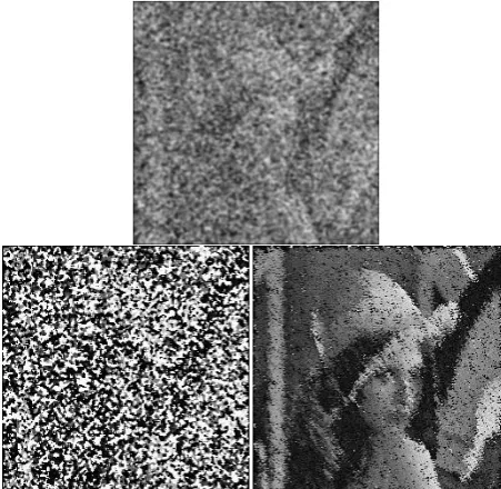
The next figure shows the result of applying Gaussian functions with different values of on the cameraman image. The increase of the standard deviation permits to accentuate filtering strength leading to remove noise but also borders. Figure number 3, shows the removed details and noise from a salt and paper noisy “Lena” image of density 0.05 by applying Gaussian filter of size (3×3).
[image:2.595.358.495.71.211.2]The main problem here is that noise, details and borders are simultaneously removed. This operation alters the image which becomes unclear and blurred.
Fig.2: Image filtering with different variances
Fig.3: Removed noise and details by a Gaussian filter.
[image:2.595.51.290.75.211.2]In order to overcome this problem we propose in this paper a Gaussian filter with dynamic structure that we call dynamic Gaussian filter “DGF”. This DGF presents a support size that varies with the magnitude of the noise and an optimal selection of the variance values instantly computed that varies proportionally with the noise intensity. In addition the convolution of this filter is applied locally on selected zones based real time computed threshold decision. Only noise is targeted, that permits avoiding as possible clean zones holding borders or details of the image.
Fig.4: Locally convolved filter with variable structure.
In fact Gaussian filter averages the noisy and noiseless pixels values to generate the output values. It cleans the image by eliminating high frequencies but affects the details and borders. The Median filter is a statistical filter that ignores impulsive noise and edge pixels when generating its output values. Consequently, there is no way that a Gaussian filter works better than a median filter when dealing with image de-noising specially if impulsive noise is used. In this paper we introduce a novel approach proposing a smart dynamic Gaussian filter with variable shape according to the image characteristics and noise intensity. To prove the superiority of the proposed filter an impulsive noise “salt and paper” is used in the tests and results are compared with the median filter known to be the most efficient tool in these conditions. Using the proposed technique we prove the image is more cleaned and its quality and details are preserved.
2. IDENTIFYING THE FILTER
PARAMETERS
We try to build up a Gaussian filter with two goals:
A variable structure and power that varies with respect to the noise intensity and locality.
[image:2.595.368.487.346.460.2]The filter parameters are instantly computes and optimized following the steps described below to give in each time a new configuration of the filter structure and shape that convolves the image on a selected zone.
2.1.
Experimental configuration
Optimal coefficients are firstly determined. Based on theses references the variation domains of the parameters that intervene in the filtering operation is determined. For that, the following steps are followed:
1. Optimal support and filter size computing. 2. Standard deviation optimization.
3. Estimation of the optimal threshold allowing applying the filter.
4. Filter convolution based on a decision computed from 8 neighborhoods comparison.
Once the optimal value for each parameter described above are computed, they are considered as references considered for the filter structure building and variation.
2.2.
Filter Size estimation
Based on [7 and 5] the optimal size of a 2D Gaussian function is
6
1
6
1
, large values of provides furtherblurring. Consequently, good silhouette images are difficult to obtain because tuning is non-trivial.
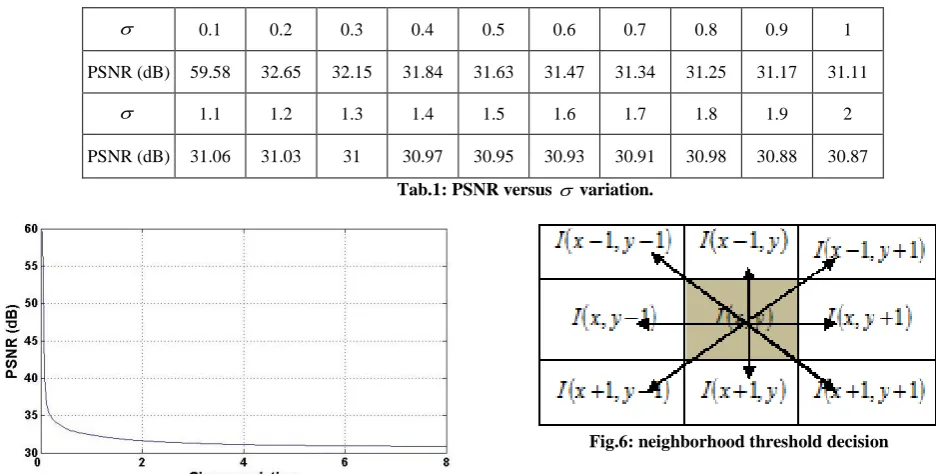
As shown by the table 1 and figure below, the tests proved that if we convolve a clean image with a Gaussian filter of this size, all the information is gathered from the value of
0
.
7
. Applying a filter with values of
0
.
7
generates a PSNR that remains practically constant in the range of 34.4 dB to 34.09 dB. This proves that the support of the Gaussian function
6
1
6
1
is enough large to contain all the data and can be trunked to this size with less data loss. The PSNR is defined as follows:
2 1 1
N i I ~ I N MSE (6)MSE
d
PSNR
2 max 10log
10
(7)Where MSE is the mean square error, dmax is the maximal coded intensity, N is the total number of pixels in the image, I and
I
are the original and filtered image. 0.1 0.2 0.3 0.4 0.5 0.6 0.7 0.8 0.9 1
PSNR (dB) 59.58 32.65 32.15 31.84 31.63 31.47 31.34 31.25 31.17 31.11
1.1 1.2 1.3 1.4 1.5 1.6 1.7 1.8 1.9 2
PSNR (dB) 31.06 31.03 31 30.97 30.95 30.93 30.91 30.98 30.88 30.87
[image:3.595.56.531.318.555.2]Tab.1: PSNR versus variation.
[image:3.595.279.520.320.543.2]Fig.6: neighborhood threshold decision
Fig.5: illustration of the PSNR variation
2.3.
Filtering with threshold decision
Traditional filtering consists in applying a convolution between the filter and all the coefficients of the image matrix leading to average the pixels values. This processes the entire image (noisy and no noisy zones). This action removes noise but also causes a general blur to the image by eliminating its high frequencies. For real applications, it’s important that the filter removes noise without damaging the image and maintains the psycho-characteristics of the processed image near to the original one. In this proposed method, the optimized filter is applied only on noisy zones avoiding all the other components of the image. Convolving the selected window is based on a decision. Every processed pixel is compared with its eight neighbors to detect high dissimilarity in pixels intensities. The filter is applied only if this dissimilarity called
I
k is detected.A threshold is fixed above witch the difference between two neighbors is considered as noise.
1 0 1 0
G , Ix ,y if I Thy , x I G Th I if y , x I y , x I k N M v v k
f (8)
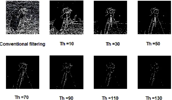
In the set of figures 8 we show the difference between the traditional filtering and a filter applied on selected zones based on a computed decision. The first figure presents the difference between the original image and the filtered one using a
3
3
Gaussian filter
G
x,
y
described by the following matrix:Fig.7: Details removed by a Gaussian filter
The second figure illustrates the removed details in the cameraman image using a locally applied filter with different
[image:4.595.237.360.69.197.2]thresholds decision Th varied respectively from 10 to 130 with a step of 10.
Fig.8: result of filtering with threshold variation
As detailed previously if the threshold is increased fewer details are removed. This is pointed up for clean image but for noisy image we have to find an optimal threshold that can remove the noise without attenuating borders and damaging details. To compute the optimal threshold, we applied the Gaussian filter on the “LENA” image with salt and paper noise of density
01 . 0
d , the threshold Th is varied from 10 to 160 and the PSNR of the filtered image is computed in each time. The decision of the best threshold is based on the PSNR and psycho-visual judgment. The table below gathers these tests results.
Tab.2: PSNR versus threshold variation.
Threshold 10 20 30 40 50 60 70 80
PSNR (dB) 34.9 35 36.5 37 38.7 39.43 40.15 40.63
Threshold 90 100 110 120 130 140 150 160
PSNR (dB) 41.18 41.71 42.16 42.5 42.8 43.2 43.7 44.2
[image:4.595.133.464.258.451.2]Figure 9a show the noisy image, figure 9b presents the filtered “LENA” image with a threshold Th=70 and sigma=0.7.
Fig.9a-b: Noisy and filtered image with optimized threshold
We conclude that more the threshold is increased less amounts of noise and details are removed. If we decrease this threshold, the filter convolves more zones of the image where one or more of the eight pixels neighbors are under this threshold when compared with the processed pixel. This causes to remove more details and noise as proved by the PSNR values. An optimal value of Th is chosen considering The PSNR variation and psycho-visual decision. If we change the noise intensity, the threshold is optimized to check the best value generating a reliable decision for filtering.
2.4.
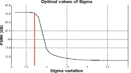
Standard deviation estimation
[image:4.595.311.533.477.574.2]noise of density d=0, 01 and an optimal threshold
Th
70
. is varied from 0 to 3 with a step of 0.1 and the PSNR is computed in each iteration.Fig.10: Result of the PSNR versus variation
.
As illustrated by the figure above the optimal standard deviation is chosen from the highest values of the PSNR. This optimal value called
o p t is injected in the first filteringiteration and is used as reference to compute in each processed window the appropriate value of the standard deviation. This computation takes into consideration the threshold
T
h andpixels variation
I
k. The following equations resume the variation of in each iteration:
h opt k v T . I Max 2 1 (9)
With
1 1
1 1 1 1 1 1 1 1 1 1 j , i I j , i I j , i I j , i I j , i I j , i I j , i I j , i I j , i I j , i I j , i I j , i I j , i I j , i I j , i I j , i I j , i Ik (10)
For k=1 to 8 “eight neighbors of each pixel”, if
I
k
Th
,
vis computed and used to define the support size of the filter. Then the shape of the filter changes in each convolution depending on the noise intensity variation. The Gaussian variable filter with its dynamic parameters and size is written as follows:
Th
I
if
Th
I
if
Th
I
Max
y
x
G
k k opt opt opt opt opt opt v Th I Max Y X1
.
2
1
,
2 2 1 2 1 1 2 2 1 6 6 6 6exp
(11)On each processed window of the image, a new Gaussian filter with specific parameters and size is applied.
3. EXPERIMENTAL RESULTS
3.1Part A
Ones the optimization procedure done, the DGF is applied on different intensities of noise. The result is firstly compared with the conventional Gaussian filter defined previously by
G
x,
y
. Since we know that with this kind of noise using the median filter is the best solution, we found that this is the best way to test our proposed filter face to high levels of noise. Many experiments are carried out with different intensities of noise. In all these tests the median filter is applied and the gathered results are compared. In each time the distortion rates and filtering results are computed and commented. In the following experiments a data base composed by 10 images is considered but only the LENA image is shown in the experimental results. 3.1.1Experiment 1In this first experiment the “LENA” image is used with a salt and pepper noise of density d=0.01 as shown in figure 11.
Fig.11: Salt and pepper noise of density 0,01.
In fact there is a strong reason for the choice of the salt and pepper noise. This impulsive noise is known to be resistant to the low-pass filter, and especially the Gaussian filter. The efficient way to remove this kind of noise is the application of statistical filters such as the median filter. This kind of mathematical filters based on a statistical approach is more efficient in this case then different low-pass filters that perform well generally in noise removing such as Butterworth with different band-widths. Although, both are applied for noise removal their behavior is different.
In the following figures we illustrate respectively a filtered image using the conventional filter and the difference resultant between the original image and the filtered one. This difference represents the amount of removed data from the noisy original image. We find that this data is composed by noise, details and borders. Since the filter convolves the entire image, no windows in the image are saved and all the high frequencies processed are subjected to be attenuated or removed. The filtered image then becomes blurred and unclear. Its PSNR is 34.79 dB.
6 In the following figures, 13a presents the noisy image
processed by the proposed DGF filter with thresholdTh40, the initial value of the optimized sigma
opt0.14. It is very [image:6.595.309.535.69.461.2]easy to perceive the difference between the two filtered images. In addition the second image showing the removed data from the noisy image prove that only noise is extracted and the details and borders are practically unchanged. This makes the filtered image more clear and understandable. The PSNR of this image is 43.12 dB.
Fig.13a-b: noisy image filtered by the proposed adjustable filter and the removed data (noise+few borders)
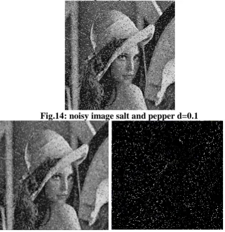
3.1.1. Experiment 2
In this experiment we augment the same noise to the density d=0.1 as shown by figure 14. Figures 15a and 15b show the noisy image filtered by the conventional Gaussian filter
3
3
,
G
x
,
y
and the correspondent removed data. The PSNR of the filtered image is equal to 31.35 dB.Fig.14: noisy image salt and pepper d=0.1
Fig.15a-b: noisy image filtered by a conventional filter.
[image:6.595.56.281.172.290.2]The following image 16a proves that using the proposed Gausian filter with adjustable dynamic structure, generates better results. This image is clearer than the filtered image using the traditional Gaussian filter. Its details and appearance are preserved. The PSNR of this filtered image is 39.13 dB that is higher than previous one. Figure 16b show that the removed data consists in noise whereas the removed data shown by figure 15b proves that the filter eliminates high frequency components that are not related only to noise but weaken sharp transitions like edges.
Fig.16a-b: noisy image filtered by the adjustable filter
3.1.2. Experiment 3
In this experiment we applied a noise which density is d=0.2.
Fig.17: noisy image salt and pepper d=0.2
Fig.18a-b: result of filtering by a conventional filter.
The PSNR of the filtered image presented by figure 18a is equal to 30.22 dB. The poor quality of this image is due to the high density of the added noise that the conventional Gaussian filter was not able to remove despite of attenuating many high frequencies coefficients. Convolving the entire image with a filter of fixed structure, damages the image quality and contributes to down the PSNR without reducing efficiently the added noise. The following figure filtered by the proposed filter, presents higher PSNR (PSNR =36.42 dB) and considerably better image quality.
Fig.19a-b: noisy image filtered by the proposed adjustable filter and the removed data.
3.1.3. Experiment 4
[image:6.595.49.276.380.614.2] [image:6.595.314.537.583.713.2]Fig.20: noisy image salt and pepper d=0.3
[image:7.595.113.226.69.183.2]The comparison result based on the computed PSNR’s between the proposed method presented by figures (22a) and the conventional approach (Figures 21a), prove the superiority of our method. The first presents a PSNR=29.74 dB whereas the second is equal to 34.78 dB. Figure 22a processed by the proposed filter presents better quality and clarity.
[image:7.595.55.284.274.507.2]Fig.21a-b: noisy image filtered by a conventional filter
Fig.22a-b: noisy image filtered by the proposed DGF filter and the removed data.
Also by comparing figures 21b and 22b we deduce that the removed data using the proposed DGF filter contains less details and borders and more noise.
3.1.4. Experiment 5
The intensity of the noise is raised up to 0,5. This level of noise covers the entire image and hides the majority of its forms and details.
Fig.23a-b-c: Three images filtered respectively by the Gaussian filter, the proposed DGF and the median filter.
[image:7.595.313.539.388.508.2]As shown by figures 23, it is clear that face to high level of noise the conventional Gaussian filter remain unable to clean it or enhance the image details that become indistinguishable. If we augment the filter size more blur is introduced to the image that can lose all its characteristics. Using the proposed method less noise resists and the forms, borders and details are evident. The following figure illustrates a comparison between the results of the proposed method, the conventional Gaussian filtering and median filtering for all densities of the used noise.
[image:7.595.160.438.552.709.2]8 It is clear that the proposed filter with dynamic Gaussian core engenders better results and more efficiency. However we tend to assume that the efficiency of the filtering operation is thresholded by the increase of noise density.
3.2.
Part B
To resolve this problem we propose in the following experiments to apply the proposed filter more than one time. Filtering many times by a low-pass filter leads to eliminate more high frequencies which damage the image and turn it unreadable. We will test if our proposed method is able to overcome this problem. The tests results are in each step commented and the distortions measurements computed. A comparison between the proposed filter, the conventional and the median filter is also conducted. The number of filtering is fixed equal to two (2). The new filter convolution is defined as follows:
1 1
1 1
x,y G , I x ,y if I Th
I G
Th I if y
, x I y , x I
k N M
n v n
v
k n
n
f
(12)
WhereIfn
x,y is the image filtered n times,
I
kis the pixelsdissimilarity engendering the filtering decision and n is the number of filtering process.
3.2.1. Experiment 1
[image:8.595.311.535.196.307.2]The first density of salt and pepper noise is d=0.01. The noisy image is filtered independently two times by the conventional filter and by the proposed one. The results are illustrated respectively by figures 25a and 25b. It is evident that the proposed method generates a filtered image visually close to the original one and very distinguishable with a PSNR =43.85 dB. All the noise was removed efficiently keeping the allure and aspect of the image unchanged. Whereas using the traditional filtering, the resulting image is blurred with a PSNR = 35.01 dB.
Fig.25a-b: Images filtered respectively by a conventional and variable Gaussian filters two times.
3.2.2. Experiment 2
Using higher density of noise reaching 0.1, the result engendered by the conventional filtering in figure 26a show a residual noise dispersed over the entire image with a low PSNR = 31.12 dB. Figure 26b proves that the proposed method allows higher performances and generates a filtered image with practically no noise. The characteristics and details of the image are preserved and it’s PSNR = 38.15 dB
Fig.26a-b: Images filtered respectively by a conventional and variable Gaussian filters two times.
3.2.3. Experiment 3
[image:8.595.311.537.342.583.2]By comparing figures 27a and 27b the difference is clearly discernible. The first figure filtered conventionally is nearly indistinguishable all the forms are vague and the noise persists ubiquitously over the whole image. The filter couldn’t remove the noise with high density (d=0.2) even though it is applied two times. The PSNR downs to 30.64 dB. Using our proposed method the image remains clear and obvious, the major part of the noise is removed without damaging the forms, the PSNR is equal to 36.48 dB.
Fig.27a-b: Images filtered respectively by a conventional and variable Gaussian filters two times.
[image:8.595.56.281.420.540.2]3.2.4. Experiment 4 The noise density is raised up to 0.4;
Fig.28a-b-c: Filtered images respectively by a conventional,
proposed filters and median filter successively two times. The figures above represent respectively the noisy image and the two filtered images with the conventional ad the proposed filter. The difference is clear and the result of the DGF is acceptable and practically exploitable.
3.2.5. Experiment 5
[image:8.595.54.279.646.747.2]Fig.29a-b-c-d: Noisy images filtered respectively by the conventional, median and variable Gaussian filters two
times.
3.2.6. Experiment 6
[image:9.595.312.538.69.294.2]Using the maximum density of noise equal to 0.9, as presented by the first figure below, the filtering process is unable to de-noise the image and separate the forms from the added de-noise. All the results generated by the filtering process of for the different noise densities are presented by figure 31.
Fig.30 a-b-c-d: Noisy images filtered respectively by a conventional, median and variable Gaussian filters two
times.
Fig.31: Comparison results between the proposed dynamic filter with the conventional and the median filter after two filtering process
3.3.
Part C
With very high level of noise we were incapable to clean the image and improve its quality even though we apply the filter two times. This leads us to increase the number of filtering process and test if the proposed filter is able to enhance the image and remedy to this problem. The problem is that this action can remove all high frequencies in the image and then turn it unreadable. On the other hand because it’s high efficiency against this noise, the comparison with median filter is conducted only for high noise densities.
3.3.1. Experiment 1
[image:9.595.148.448.398.566.2]10
Fig.32 a-b-c-d: Noisy images filtered respectively by a conventional, median and variable Gaussian filters three times.
3.3.2. Experiment 2
[image:10.595.311.537.72.292.2]Even though with a noise of density equal to 0.7, when compared with the median or conventional filtering, excellent results are generated using the variable dynamic filter with Gaussian core. The results are shown by figures 33a, 33b and 33c. It is obvious that our proposed filter gives better de-noising results than the median filter that is known to be the most efficient against this type of noise. The forms and details are kept practically clear.
Fig.33 a-b-c: Noisy images filtered respectively by a
conventional, median and variable Gaussian filters three times.
3.3.3. Experiment 3
Basing on the literature for different kinds of low-pass filtering, it is impossible to correct, improve and clean this high level of noise. Only our proposed dynamic filter with variable structure was able to clean and determine the forms and some details of the processed image generating the correct allure. The following images illustrate the filtering results with a salt and paper noise of density 0,9. The PSNR variation of the filtered image for different noise densities (From 0.1 up to 0.9) is illustrated in figure 35.
Fig.34 a-b-c: Noisy images filtered respectively by a conventional median and variable Gaussian filters three times.
[image:10.595.133.465.427.536.2] [image:10.595.146.454.560.729.2]3.4.
Part D
We are interested in this section by testing our DGF with high number of filtering process against only higher densities of noise. We apply only strong noises that make the image unreadable and indistinguishable. All the carried tests are compared with conventional and median filtering. The same noise is used in these experiments presented by its density d, the number of filtering applications is equal to four (04).
3.4.1. Experiment 1
[image:11.595.311.537.71.182.2]From the following figures, it’s very clear that the median filter was not able to clean image attacked by very high level of noise despite its high efficiency. The results shown by figures 36d prove that even with very high density of noise the filtered image using the proposed filter is enhanced and its quality is improved basing on four successive filtering. It is too interesting to discover that more the number of filtering is high more the image is cleaned and improved. These improvements occur without damaging the details such as with conventional filter. The density of the noise d=0.8.
Fig.36 a-b-c-d: Noisy images filtered respectively by a conventional, median and variable Gaussian filters four times.
3.4.2. Experiment 2
The maximum density of noise is applied in this step (d=0.9). The following figures illustrate respectively the noisy image, the filtered images respectively with conventional Gaussian filter, median filterer, and the proposed adjustable filter with Gaussian core. The results do not need any comments. The proposed method supplies visually better results and the image details are discernible. The comparison results illustrated by figure 38 prove that the quality of the processed image using the proposed method is visually better and higher PSNR. Figures 38 illustrate the comparison results of the PSNR variation between the different filtering methods.
Fig.37a-b-c-d: Noisy images filtered respectively by a conventional, median and variable Gaussian filters four times.
Fig.38: Comparison results between the proposed and the conventional filter after four filtering passages
[image:11.595.53.507.264.694.2]12
Tab.3: Comparing the PSNR’s results of the different filters: the conventional Gaussian filter, the median filter and the proposed Gaussian variable filter.
Noise density
0.1 0.2 0.3 0.4 0.5 0.6 0.7 0.8 0.9
PSNR (dB)
1st filtering
D.G.F.V.S 39.13 36.42 34.78 32.24 31.27 30.25 29.58 29.42 28.69
C.G.F 31.35 30.22 29.74 29.68 29.47 29.5 29.16 28.86 28.11
M.F 32.52 31.13 30.07 28.9 28.15
2nd filtering
D.G.F.V.S 38.15 36.48 34.10 32.25 31.60 30.42 29.82 29.53 29.03
C.G.F 31.12 30.64 30.15 30.12 29.87 29.40 29.01 28.53 28.12
M.F 30.21 29.63 28.84 27.68 27.1
3rd filtering
D.G.F.V.S 33.77 32.10 31.71 30.95 30.44 30.14 29.96 29.29 29.01
C.G.F 31.05 30.81 30.30 30.21 29.77 28.73 28.64 28.31 28.12
M.F 30.05 28.98 28.73 28.32 28.10
4th filtering
D.G.F.V.S 33.83 33.50 33.49 34.07 33.88 31.81 30.76 29.71 29.21
C.G.F 30.99 30.88 30.36 30.36 30.11 30.12 29.04 28.61 28.52
M.F 31.97 30.4 29.82 29.16 28.77
The D.G.F.V.S represents the dynamic Gaussian filter with variable structure, the C.G.F is the conventional Gaussian filter and the M.F is the median filter.
The superiority of the proposed method is well illustrated in table3. For the same density of noise and in each experiment the proposed method allows better filtering and higher image quality.
4.
CONCLUSION
In this paper a novel technique of filtering is presented. Using a dynamic Gaussian filter with variable structure as core of convolution, the filtered image is enhanced even if very high density of noise is used. The proposed technique avoids convolving the filter on the whole image. In each processed windows a comparison procedure ended by a decision, judges if the filter must be applied or not. This procedure allows removing only the noise and avoids extracting details or borders which generates clear image even if the filter support is too large or the filter is applied several times. As well depending on the intensity of the detected noise, all the structure of the Gaussian filter is continuously changed by computing and updating in real time the required parameters .The appropriate size of the filters and its strength are optimized and then iteratively computed to remove efficiently noise. In the other hand, the proposed filter conserves the image details and borders exactly as the median filters acts. In this work essential advantages are developed:
Applying the proposed filter many times generates excellent results without damaging the image quality or altering its forms specially when dealing with higher densities of noise.
Despite the specific efficiency of the median filter to remove salt and paper noise and the deficiency of the conventional Gaussian filter against this kind of impulsive noise, the proposed filter generates better results specially when dealing with high levels of noise densities.
The shape variability of the proposed filter allowed it to be adjustable for many kinds of noise.
The choice of a Gaussian model as filter core is based on its capacity to conserve more details and borders then other filters. In addition it considers better the correlation between the pixels in the image and especially for textures, that’s why textures are generally represented by Gaussian models.
In the end this proposed approach combines the behavior of an intelligent dynamic low-pass filter that eliminates only high frequencies corresponding to noise and a filter based statistical approach that removes efficiently impulsive noise and conserves details and borders unchanged.
The results prove that the proposed filter escape to the high blur introduced by a static Gaussian filter and exceeds the results of a median filter especially when dealing with high densities of noise
5. REFERENCES
[1] M. Basu, “Gaussian-Based Edge-Detection Methods—A Survey”, IEEE Transaction on systems, man, and cybernetics—part C: application and reviews, VOL. 32, NO. 3, August 2002.
International Conference on Computer Vision Theory and Applications, - Volume 2, February , 5-8, 2009 , Lisboa, Portugal.
[3] J. Bobud, A.P. Withkin, M. Baudir and R.O. Duda, “Uniqueness of the Gaussian kernel for scale space filtering”, IEEE Trans. PAMI, vol. 8, n°1, pp. 26-33, 1986.
[4] J.M. Geussenbroek, A.W.M. Sneulders, J.V. Weiger,” fast anisotropic Gaussian filter”, IEEE Trans. On Image processing, Vol12, N°8, pp. 938-943, August 2003.
[5] D. Hale, “ Recursive Gaussian filter”, Report, Center for Wave Phenomena, Colorado School of Mines, USA (2006).
[6] I. T. Young, L.J. Van vliet, “Recursive implementation of the Gaussian filters”, Elsevier, Signal processing (44),
[7] Q. Kemao, “On window size selection in the windowed Fourier ridges algorithm”, Elsevier, Optics and Lasers in Engineering 45 (2007) 1186–1192.
[8] R. Sznitman, “Reducing the error rate of a Cat classifier”, international conference in information visualization, IV 2007, 2-6 July 2007, Zürich, Switzerland. IEEE Computer Society 2007.